Do Type-Ia Supernovae Constrain the Total Equation of State?

Abstract

In this paper, we consider a couple of alternative dark energy models using the total equation of state of the cosmological fluid, $w_{tot}$. These models are fit to the recent type-Ia supernovae data and are compared to previously considered models. The first model is based on the hyperbolic tangent and provides a good estimate of the rate of the transition to dark energy domination. The second model is a cubic spline model. This model demonstrates and quantifies the non-monotonicity in the total equation of state coming from the supernovae observations. At present, the supernovae observations indicate significance to non-monotonically decreasing dark energy. We derive constraints on the spline paramters and compare and constrast the results to the Cosmological Constant dark energy model. Both the hyperbolic and splines models indicate that a precise physical notion of dark enegy is a potentially ever more mysterious quantity?

I Introduction

Observations of distant type-Ia supernovae have shed great light on the evolution of universe at late timesP98 ; k03 ; Riess98 ; Riess01 ; Riess04 ; R06 . These observations indicate that the universe is presently undergoing an accelerated expansion that started about 7 billion years ago. The source of this acceleration has been labeled dark energy and the corresponding energy density is peculiar in that it appears to require a negative equation of stateStaro03 . Cosmologists were quick to pursue models which reproduce the observed effects of the dark energy. All of these models have negative equations of state coming from positive dark energy density and negative pressure.

The first of these models has its historical origins with Einstein. It is the Cosmological Constant Cold Dark Matter (LCDM) cosmological model. This model adds an additional constant $\Lambda$ to the Einstein Equations. The resulting model of dark energy is typically characterized by a constant equation of state $w_{\Lambda}\equiv P_{\Lambda}/\rho_{\Lambda}=-1$. Initially, the LCDM model fit observational data quite wellRiess98 ; P98 . More recent data suggests that while this model is not ruled out, it is statistically not as favored as models with smaller constant equations of stateRiess04 ; Caldwell02 . Still, others propose to introduce phenomenological models of the dark energy equation of state (and consequently the energy density) based on kinematicsGong04 or linear Taylor’s Series expansions of the dark energy equation of state ($w_{V}$) Turner02 ; Linder03 ; Riess04 . The latter model was shown to be divergent at early times and has since fallen out of favor. However, this inspired others to introduce alternative evolving dark energy equations of state which removed the early time exponentially divergent behaviorLinder05 ; padman05 . The first example of these models was originally proposed by Chevalier00 as an alternative to constant equation of state models and has an evolving equation of state. In padman03 , they use this model to analyze different properties of the supernovae data and implications for the dark energy parameters. For dark energy, they find that it is difficult to tightly constrain several dark energy parameters using the recent supernovae data.

In Staro03 , they propose several ansatz models for the hubble parameter which are polynomials of the cosmological scale factor. In these models, the dark energy is characterized by an equation of state that metamorphosizes from $w_{V}=0$ at a redshift $z>1$ to $w_{V}\approx-1$ at $z=0$. From this analysis, they conclude that the supernovae data favors negative evolving equations of state for dark energy. Similar ansatz models for dark energy were proposed in Odintsov and are consistent with the results from Staro03 . Still others have proposed modeling dark energy equation of state by using cubic splinesWang04 . Here, they constrain dark energy in a series models and find that they are consistent with negative equations of state using supernovae, gravitational lensing and large scale structure. The results of their analysis put tight constraints on dark energy equations of state.

A very curious set of models are the Sudden Gravitational Transition models, see Caldwell05 and references therein. These models suppose that dark energy is the result of a late-time phase transition in the universe. The source of the dark energy is the result of a resonant effect of a free, ultra-low mass, quantized scalar field coming from Quantum Field Theory in Curved Spacetime. With a suitably chosen order parameter $\eta$, this resonance causes $\eta\rightarrow\chi^{2}m^{4}={\rm constant}$ where $\eta$ takes the form $R^{2}$, $R_{\mu\nu}R^{\mu\nu}$ and $R_{\mu\tau\nu\rho}R^{\mu\tau\nu\rho}$. The model for which $\eta=R^{2}$ is called the Vacuum Cold Dark Matter (VCDM) cosmological modelParker99a ; Parker99b ; Parker00 ; Parker01 ; Parker04 . In all of the Sudden Transition models, the effects of the scalar field are negligible until about half the age of the present universe, denoted in terms of redshift as $z_{j}$ and is labeled the redshift of transition. Here $\chi^{2}m^{4}$ is the one free parameter of these models with $\chi$ corresponding to a dimensionless parameter fixed by the theory and $m$ is the mass of the scalar field. The constant $\eta$ arising from this effect reacts back on the universe which results in an accelerated expansion through a sort of gravitational Lenz’s law. It has been shown that these types of models are tightly constrained by the recent cosmological experimental data, see Caldwell05 ; komp04 ; ckpv2005 ; pkv2003 for details.

The effects of these models are different than the previous ones in that they change the nature of gravity itself. Dark energy is not an unknown extra quantity that appears in the total energy density $\rho_{tot}$ but is a manifestation of the changes in gravity induced by the effects of the field. However, these changes lead to comparable results to the previous dark energy modelsckpv2005 ; Caldwell05 ; komp04 .

A similar model to the Sudden Gravitational Transition models is the Super-Acceleration modelonemli02 ; onemli04 . This model is based on Quantum Field Theory in Curved Spacetime as well. A fully renormalized energy density and pressure are computed for a scalar field with a quartic self-interaction in a locally De Sitter spacetime. The resulting cosmology leads to a dark energy term in the Einstein equations which has a dark energy equation of state which relaxes gradually from 0 to -1.

What we propose here is that we model directly the Hubble parameter’s evolution through the total equation of state $w_{tot}$. This is similar to the method from Staro03 mentioned above. This approach has a novelty that it does not have the present day matter density $\Omega_{m0}$ (or alternatively the present day dark energy density $\Omega_{X0}$) as a free parameter and models directly the kinematics contained in the supernovae data, see Staro03 ; padman03 for nice discussions. We will take two approaches to the modeling. The first approach is based on a phenomenological model that was inspired by the hyperbolic tangent, hence forth labeled the hyperbolic model. This model has two parameters which determine the time of transition ($\alpha$) and the strength of transition ($\beta$). This 2 parameter model is fit to supernovae data using a finite linear grid and marginal parameter estimates are extracted using the procedure discussed in komp04 . When suitably tuned by this fit, these parameters cause $w_{tot}$ to undergo a transition that will cause it to deviate from 0 at a redshift $z\approx 1$. This transition is a monotonically decreasing function of time bounded below by -1 or conversely a monotonically increasing function of redshift bounded above by 0.

For simplicity, we have set the amplitude of the transition to unity. This sets the cosmology to asymptote to de Sitter spacetime, i.e. $w_{tot}$ asymptotes to $-1$. This is motivated from the results presented in Wang04 , where they show that the supernovae data does not constrain the dark energy density for redshifts $z<0$. If some data in the future becomes available to constrain the dark energy at these redshifts, then it is possible to adjust the amplitude and it would become an additional parameter. We will show that the transition in this model is very reminiscent of the models of dark energy discussed above and in particular behaves most like the Sudden Gravitational Models and the dark fluid modelArbey05 .

The second approach to modeling $w_{tot}$ that we will take is a phenomenological cubic spline analysis. Our interests are to constrain cubic spline models of $w_{tot}$ to the ranges of redshift associated with dark energy domination between redshifts ($0<z<1$). We choose two different uniform densities for the splines, consisting of 3 and 6 points. The spline points correspond to the model parameters and will be denoted as $a_{i}$ for $i=1,2,3$ for the 3-point model or $i=1,...,6$ for the 6-point model.

We choose to vary the spline points over a finite uniform linear grid. Performing the fit to the supernovae data at each point. From this analysis, we conclude that the supernovae data favors not just monotonically decreasing $w_{tot}$ with one extremal point, but allows (and marginally favors for some data sets) transitions which have several extremal points. However, implications for monotonically decreasing $w_{tot}$ shows that the results of the various proposed models above are within the constraints allowed by the spline analysis.

Both of the cosmologies proposed in this paper have an earlier matter dominated epoch followed by a later dark energy dominated epoch (i.e. $w_{tot}=0$). In the earlier matter dominated epoch, the energy density which would characterize this later epoch appears as (presumably) cold (presumably) dark matter like some of the models considered in Staro03 . Thus, these models have some subset of dark matter which undergoes a transition to dark energy. This transition is similar to the dark fluid model presented in Arbey05 . There, he supposes that the riddle of dark energy and dark matter are one in the same. Dark Matter begins to undergo some transition, like a decay, into dark energy at $z\approx 1$.

In section II, we will propose the two models of $w_{tot}$ and fit them to the recent supernovae data. One is a toy model based on the hyperbolic tangent and the other is a cubic spline model. In section III, we will discuss comparison of the models considered in the previous section to the LCDM model. Also, comparison of the models to the recent WMAP data through the shift parameter will be discussed.

In section IV, we will summarize our results and make concluding remarks about these two models and compare them to the LCDM model. It should be noted that implicit in this discussion is the Friedmann-Robertson-Walker (FRW) spacetime invariant line element given by

$$ds^{2}=-dt^{2}+a^{2}(t)\left(\frac{dr^{2}}{1-kr^{2}}+r^{2}(d\theta^{2}+\sin^{2}(\theta)d\phi^{2})\right)\;,$$ (1)

where $k$ specifies the curvature of the spatial hypersurfaces in spacetime. In this paper, we will assume spatially flat hypersurfaces, i.e. $k=0$. Also, we assume that the energy-momentum-stress tensor is given by a perfect fluid with total energy density ($\rho_{tot}$) and pressure ($P_{tot}$).

II Modeling Dark Energy

Typically, cosmologists interpret the observed late-time acceleration as arising out of some non-standard cosmological energy density. In order for this energy density to achieve the observed acceleration, it needs to exert a significant negative pressure at late times in the universe’s evolution. This means that the ratio of pressure to energy density (presumed to be non-negative) is negative, i.e. the dark energy equation of state $w_{V}(z)=P_{V}/\rho_{V}<0$. All reasonable fitting dark energy models are in agreement on this point. For the LCDM model, $w_{V}(z)$ is equal to $-1$ for all redshifts. For the VCDM model and the other sudden gravitational transition model pkv2003 ; komp04 ; Caldwell05 , $w_{V}(z)$ is shown to be less than $-1$ for late-times after the transition to dark energy domination. Similarly in Linder05 ; Wang04 ; padman05 , they consider a significant number of dark energy models and find $w_{V}(0)<0$ is favored.

With this in mind, we propose to model dark energy with no explicit dependence on $\Omega_{m0}$ by using the total equation of state of the universe $w_{tot}$ given by

$$w_{tot}=\frac{P_{tot}(z)}{\rho_{tot}(z)}\;,$$ (2)

where $P_{tot}(z)$ and $\rho_{tot}(z)$ are the total pressure and energy density of the universe respectively. The benefit of this approach of modeling the effects of dark energy is that at late times any parameters introduced into (2) which cause $w_{tot}$ to become negative correspond to dark energy parameters. Previously, one had the parameter $\Omega_{m0}$ with which to contend and when combined with other data would put constraints on fitting to the supernovae observations. We will constrain the empirically permissible deviations from a Standard Cold Dark Matter model. It should be noted that one could assume this approach and arrive at all of the expressions for $w_{V}(z)$ arising out of the various dark energy models. So, this approach changes nothing for the previous models but allows for a new angle of examination of the supernovae observations which can be compared and contrasted to models that have already been examined.

Now, assuming the invariant line element in (1), then the time-time Einstein Equation is given by

$$\frac{H^{2}(z)}{H^{2}_{0}}=\frac{8\pi G}{3H_{0}^{2}}\rho_{tot,0}\frac{\rho_{tot}(z)}{\rho_{tot,0}}\;,$$ (3)

where $H^{2}_{0}$ is the present day hubble constant and $\rho_{tot,0}$ is the present day value of the total energy density. We are assuming a spatially flat universe. Thus,the total energy density $\Omega_{0}\equiv(8\pi G)/(3H_{0}^{2})\rho_{tot,0}=1$. Substituting this result into (3) gives

$$\frac{H^{2}(z)}{H^{2}_{0}}=\frac{\rho_{tot}(z)}{\rho_{tot,0}}\;.$$ (4)

Assuming $T^{\mu\nu}$ is a perfect fluid, $\nabla_{\mu}T^{\mu\nu}=0$ implies that $\frac{\rho_{tot}(z)}{\rho_{tot,0}}$ satisfies the following expression

$$\frac{\rho_{tot}(z)}{\rho_{tot,0}}={\rm Exp}\left[3\int_{0}^{z}\frac{dz^{\prime}}{1+z^{\prime}}(1+w_{tot}(z^{\prime}))\right]\;,$$ (5)

where we have explicitly written the redshift dependence of $w_{tot}$.

From this equation, we can see that modeling $w_{tot}$ is directly modeling the hubble parameter, (4), which is the method used in Staro03 . So in this paper, we are presenting alternative models of the hubble parameter.

II.1 The Hyperbolic Model

Now, lets suppose a particular phenomenological model of $w_{tot}$ which will characterize the transition to dark energy domination. This model is inspired by the hyperbolic tangent function and will be labeled the hyperbolic model. We will assume a prior matter dominated epoch for $z\approx 1$ and above, i.e. $w_{tot}=0$. As discussed above in order to get a dark energy model with late-time negative pressure, $w_{tot}$ must become negative as $z$ goes to 0 (present day). Let $w_{tot}$ be defined by

$$w_{tot}=-\frac{{\rm Exp}[-\beta(z-\alpha)]}{{\rm Exp}[-\beta(z-\alpha)]+{\rm Exp}[+\beta(z-\alpha)]}\;,$$ (6)

where $\beta$ and $\alpha$ are labeled as transition parameters. $\beta$ controls the strength of the transition to dark energy dominated epoch and $\alpha$ controls the time of transition.

Substituting (6) into (5), we get

$$\frac{\rho_{tot}(z)}{\rho_{tot,0}}={\rm Exp}\left[3\int_{0}^{z}\frac{dz^{\prime}}{1+z^{\prime}}\left(1+\frac{{\rm Exp}[-\beta(z^{\prime}-\alpha)]}{{\rm Exp}[-\beta(z^{\prime}-\alpha)]+{\rm Exp}[+\beta(z^{\prime}-\alpha)]}\right)\right]\;.$$ (7)

Substituting this expression into the time-time Einstein equation (4) gives the following expression for the hubble parameter for this phenomenological model

$$\frac{H^{2}(z)}{H^{2}_{0}}={\rm Exp}\left[3\int_{0}^{z}\frac{dz^{\prime}}{1+z^{\prime}}\left(1+\frac{{\rm Exp}[-\beta(z^{\prime}-\alpha)]}{{\rm Exp}[-\beta(z^{\prime}-\alpha)]+{\rm Exp}[+\beta(z^{\prime}-\alpha)]}\right)\right]\;.$$ (8)

Now, we fit to the experimental data from R04 and SNLS through the luminosity distance following the $\chi^{2}$ procedure given in ckpv2005 ; komp04 using (8) to give the hubble parameter as a function of redshift.

Performing this fit, we get the results presented in table 1. The first column corresponds to the data set(s) used in the fitting. The second column corresponds to the local minimum in $\chi^{2}$. The last two columns correspond to the marginal parameter estimates and uncertainties of $\alpha$ and $\beta$. The resulting fits for each data set are marginally better than for the LCDM model. Also, the transition and evolution of the dark energy appears to favor a greater negative pressure consistent than that which the LCDM model favors. This is shown for each data set in figure 1.

$\begin{array}[]{ccc}\includegraphics[width=144.54pt]{R04phenwtot.eps}&\includegraphics[width=144.54pt]{snlsphenwtot.eps}&\includegraphics[width=144.54pt]{jointphenwtot.eps}\\ \includegraphics[width=144.54pt]{R06phenwtot.eps}&\includegraphics[width=144.54pt]{jointR06phenwtot.eps}&\end{array}$

Figure 1: Plots of the $w_{tot}$ and 2$\sigma$ confidence region for the hyperbolic dark energy model given by (6) for the supernovae data sets R04, R06, SNLS, R04+SNLS and R06+SNLS data sets. The solid curves in each graph correspond to the marginal estimate for $\alpha$ for each data set presented in table 1. The dashed lines correspond to the uncertainty in $\alpha$. For these graphs, we set $\beta=3$ which is near the center of the ranges given in the table. From the graph, this model starts out asymptotically in a matter dominated stage,$w_{tot}=0$. As $z\rightarrow 1$, the dark energy becomes significant driving $w_{tot}$ negative. This model by construction asymptotes to a LCDM model as $z\rightarrow-1$.

From this figure, the transition to dark energy domination ($z_{j}$) occurs at $z\approx 1$ and is smooth like the LCDM. From the fit to the supernovae data, this redshift is smaller than the corresponding redshift of transition for the LCDM model. However, the hyperbolic dark energy increases very rapidly and quickly dominates the energy density in the Einstein Equation (4). So, while the hyperbolic dark energy model near $z_{j}$ is smooth like the LCDM, the transition of the dark energy is more akin to the Sudden Gravitational TransitionCaldwell05 and Dark Fluid ModelArbey05 .

Table 1: A table of the marginal parameter estimates of the hyperbolic model derived from the R04, R06 and SNLS data at $2\sigma$.

Data Set	$\chi^{2}_{{\rm min}}$	$\alpha$	$\beta$
R04	175	$0.25\pm 0.08$	$7.0^{+8.0}_{-7.0}$
SNLS	62	$0.37\pm 0.10$	$2.1^{+2.8}_{-2.0}$
R04+SNLS	238	$0.29\pm 0.08$	$3.4\pm 3.2$
R06	201	$0.26\pm 0.08$	$6.3\pm 5.0$
R06+SNLS	264	$0.29\pm 0.07$	$3.2\pm 2.8$

From table 1, the $\alpha$ parameter is constrained and $\beta$ appears weakly constrained. However, the trend from this table is that the most recent supernovae observations are beginning to provide additional information which results in tighter constraints on cosmological parameters. Thus, the supernovae data only constrains one of our transition parameters. In figure 1, we see a plot of the 2$\sigma$ confidence region for $w_{tot}$ coming from the marginal estimates and uncertainties. This is in agreement with Linder05 ; Wang04 ; Gong04 ; Caldwell05 ; komp04 , where they show from the analysis of many models that only one parameter of dark energy is constrained by the data. This also agrees with the results obtained below in section III.

In Chevalier00 ; Linder05 , their analysis assumed particular forms of the dark energy density ($\rho_{V}(z)/\rho_{V}(0)$) with the constrained parameters roughly corresponding to the dark energy equation of state $w_{V}(z=0)$ and $w^{\prime}_{V}(z=0)$. One of the simplest model is of the form

$$w_{V}(z)=w_{0}+w_{1}\frac{z}{1+z}\;,$$ (9)

where $w_{0}$ and $w_{1}$ are both parameters of the modelChevalier00 . This model has been labeled as model 2.0 in Linder05 . We will assume this label here.

In Wang04 , they used spline approximations of the dark energy equation of state. We will consider a similar model below. In Gong04 , he assumed a kinematic expansion of the cosmological scale factor up to the snap term ($\propto\ddddot{a(t)}$). The Sudden Gravitational Transition models from Caldwell05 assumed a spatially flat universe where the one free model parameter corresponds to $\Omega_{m0}$. This parameter was found to be tightly constrained. However, if one introduces curvature, $\Omega_{m0}$ is found to have a high degree of covariance with $\Omega_{k0}$ which is not tightly constrainedkomp04 . This result is similar to that shown in figure 4 of padman03 .

A comparison plot of several of these models and the hyperbolic one is given in figure 2.

Figure 2: (color online) A comparison plot of $w_{tot}$ for various dark energy models. The light blue curve corresponds to the linear Taylor’s Series model from R04, with parameters $\Omega_{m0}=0.27$, $w_{0}=-1.3$ and $w^{\prime}_{0}=1.5$. The green curve corresponds to the Linder 2.0 model (defined by (9)) with parameters $w_{0}=-2.25$ and $w_{1}=0.3$. The purple curve corresponds to the N=4 VCDM model with $\Omega_{m0}=0.45$. The dashed curve corresponds to the LCDM model with $\Omega_{m0}=0.27$. The solid black curve is the phenomenological model presented in this paper with $\alpha=0.25$ and $\beta=3$.

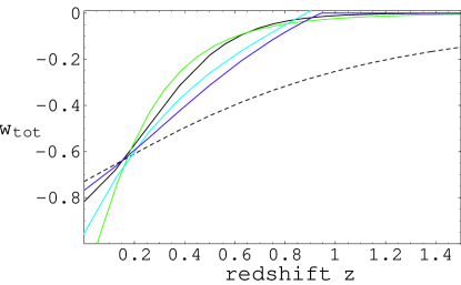
From this figure, we see that all of the models appear to converge in their prediction of $w_{tot}$ at $z\approx 0.19$. Thus at this redshift, the supernovae predicts that $w_{tot}\approx-0.6$. Notice that the Linder 2.0 model and the Linear Taylor’s Series model have divergences. The former diverging in the distant future of $z=-1$ and the latter diverging at $z=-1$ and $z\rightarrow\infty$. The hyperbolic model proposed here has no such divergences and most closely resembles the VCDM model (Parker04 and references therein) and the dark fluid model of Arbey05 .

From the early redshift behavior, it would appear that this model suffers from a similar divergence problem as the linear Taylor’s Series model used in Riess04 ; komp04 , but this is not the case. Upon inspection of (5), one sees that $w_{tot}$ vanishes for $z\approx 1$ and greater. This means that during the preceding matter dominated stage, this form of dark energy behaves just like pressureless non-relativistic matter, i.e. grows as $(1+z)^{3}$ and has an equation of state $w_{V}=0$. Thus, this dark energy model is some form of the dark fluid from Arbey05 and the ansatz models from Staro03 . For $z>1$, $\Omega_{V}(z)(\equiv 8\pi G\rho_{V}(z)/(3H_{0}^{2}))$ is given by

$$\Omega_{V}(z)\approx\left(\Omega_{Vj}-\Omega_{m0}\right)(1+z)^{3}\;,$$ (10)

where $\Omega_{Vj}$ is some constant determined by $w_{tot}$ at the redshift of transition ($z_{j}$) which is a function of $\beta$ and $\alpha$. For typical values of these two parameters coming from fitting to the supernovae data (below), $\Omega_{Vj}\approx 1.5\Omega_{m0}$. Thus at early time, this form of dark energy would only make the universe appear that it has more cold matter than it really does. This is the essence of the dark fluid model where dark energy arises out of dark matter around the transition at $z=z_{j}$. We can compare the hyperbolic model to the other dark energy models by introducing the assumption that $\rho_{tot}=\rho_{m}+\rho_{V}$ where $\rho_{m}$ and $\rho_{V}$ are the energy densities of matter and dark energy respectively. Upon inspection of (6) and (5), $\rho_{V}$ for the hyperbolic model is present at all stages of the universe’s evolution, which is a trait that it has in common with the LCDM model. To make a quantitative accessment, it is necessary to assume a value for the ratio of the matter energy density to critical density at present day, $\Omega_{m0}\equiv 8\pi G\rho_{m0}/(3H_{0}^{2})$. Since the hyperbolic model most closely resembles the VCDM model, we will assume that $\Omega_{m0}=0.45$ which is the marginal estimate from that model. As shown in figure 3, the dark energy density associated with the hyperbolic model decreases as z approaches 1 from above behaving as matter, $\rho_{V}\propto(1+z)^{3}$. At $z\approx 1$, the dark energy evolution begins to deviate from $(1+z)^{3}$ and begins to grow in significance. This is where the negative pressure from the dark energy begins to grow resulting in the observed acceleration. This is indicated by the increase at low redshift in the figure.

Figure 3: A comparison plot of the predicted ratio dark energy density to its present day value versus redshift (upper) and the dark energy equation of state (lower) for the phenomenological model with $\alpha=0.29$ and $\beta=3.0$ assuming $\Omega_{m0}=0.45$ (solid curves) and the LCDM model (dashed curves). At increasing redshift this model indicates that the energy density of the universe is behaving identical to that of non-relativistic matter. Approaching present day, this decreasing energy density reaches a minimum a begins to increase again. This is reminiscent to the effects which occur in the Sudden Gravitational Transition modelsCaldwell05 , the dark fluid model proposed in Arbey05 and the ansatz models from Staro03 . Clearly, the data allows for physical models which have significantly different dynamics.

The behavior of this equation of state is reminiscent of the Sudden Gravitational model with a non-zero cosmological constantCaldwell05 and the dark fluid model Arbey05 .

In this section, we have shown that the hyperbolic model fits to the supernovae data quite well as compared to the other cosmological models. In the next section, we generalize the approach of using $w_{tot}$ by using spline approximations, similar to those used in Wang04 . We have fixed by construction that this model asymptote to a LCDM model as $z$ goes to $-1$. However, one could introduce a non-unit amplitude in the numerator of (6) and have it asymptote to any value. However, introducing this parameter would increase this model to a 3 parameter model. Given that the supernovae data constrains only one of the two parameters, introducing a third would most likely not the statistical significance of the model to the supernovae data.

II.2 Spline Approximation

In this section, we will use cubic splines to approximate $w_{tot}$. This is similar to the analysis performed in Wang04 . There they modeled the dark energy equation of state $w_{V}(z)$ using cubic splines. The analysis in this paper will assume a prior matter dominated stage ending at $z\approx 1$. Thus, we will assume that the spline points of $w_{tot}$ for redshifts $z>1$ vanish. The model parameters of these spline models are the spline points that specify the spline functions for $z\leq 1$. Recall from the hyperbolic and other dark energy models considered in section II.1, we found that the dark energy effects become significant near the redshift of transition, $z_{j}$. We want to use the splines to try and constrain what types of transition and evolution of the dark energy from $z_{j}$($\approx 1$) to present day. Thus, the redshifts of the parameters of the spline model will be contained in the redshift interval [0,1]. In this interval, we will analyze uniform grids of spline points. Consider two densities of spline points, 3-point and 6-point, which will be denoted as $a_{i}$ for i=1-3 or 1-6. Our main interest here is constraining $w_{tot}$ using the supernovae data, inferring properties of $w_{tot}$ and comparing the results to other models. We will show that the computed confidence regions of the splines models will have significant intersection with most of those from the dark energy models discussed in section II.1.

Assuming that $w_{tot}$ is given by a cubic spline function, we can fit the resulting cosmological models using the same $\chi^{2}$ procedure that was used for the hyperbolic model. Fitting to the data, we find the minimum $\chi^{2}$ and marginal estimates for the 3 point spline is present in table 2 and for the 6 point spline is present in table 3.

Table 2: Marginal Parameter estimates at 2$\sigma$ and the minimum $\chi^{2}$ for the 3 point spline model with parameters $a_{1}$, $a_{2}$ and $a_{3}$.

Data Set	$\chi^{2}_{{\rm min}}$	$a_{1}$	$a_{2}$	$a_{3}$
R04	174	$-0.5^{+0.5}_{-0.6}$	$-0.4\pm 0.2$	$-1.3\pm 0.5$
SNLS	62	$-0.3^{+0.3}_{-0.4}$	$-0.6\pm 0.1$	$-0.7\pm 0.4$
R04+SNLS	238	$-0.4\pm 0.2$	$-0.6\pm 0.1$	$-0.8\pm 0.3$
R06	200	$-0.5\pm 0.2$	$-0.4\pm 0.2$	$-1.3\pm 0.5$
R06+SNLS	262	$-0.4\pm 0.2$	$-0.6\pm 0.1$	$-0.7\pm 0.4$

Table 3: Marginal Parameter estimates at 2$\sigma$ and the minimum $\chi^{2}$ for the 6 point spline model with parameters $a_{1}$, $a_{2}$, $a_{3}$, $a_{4}$, $a_{5}$ and $a_{6}$. We find that the either or both supernovae data sets have wide marginal distributions for the the parameters $a_{1}$ and $a_{2}$ and thus does not offer significant constraints. Subsequently, we will not list them in the table below. As well, we find that the R04 data does not constrain $a_{3}$. The SNLS data constrains only two parameters $a_{4}$ and $a_{5}$. Together, both data sets constrain $a_{3}$, $a_{4}$, $a_{5}$ and $a_{6}$. Unconstrained parameters are denoted by dashes in the table. All uncertainties are at 2$\sigma$. Notice that the R06+SNLS minimum $\chi^{2}$ is greater in the 6 point model than in the 3 point model. This is due to parameter space grid is more dense than in the 3 point model. Computational time was too prohibitive to fill in the grid to the same density as was done for the 3 point model.

Data Set	$\chi^{2}_{{\rm min}}$	$a_{3}$	$a_{4}$	$a_{5}$	$a_{6}$
R04	174	–	$-0.3^{+0.3}_{-0.5}$	$-0.6^{+0.4}_{-0.4}$	$-0.9^{+0.5}_{-0.5}$
SNLS	61	–	$-0.5^{+0.5}_{-0.6}$	$-0.6^{+0.4}_{-0.4}$	–
R04+SNLS	237	$-0.3^{+0.3}_{-0.6}$	$-0.4^{+0.4}_{-0.6}$	$-0.6^{+0.4}_{-0.4}$	$-0.9^{+0.6}_{-0.6}$
R06	200	$-0.2^{+0.2}_{-0.6}$	$-0.1^{+0.1}_{-0.4}$	$-0.7\pm 0.4$	$-0.3^{+0.3}_{-0.4}$
R06+SNLS	264	$-0.2^{+0.2}_{-0.4}$	$-0.3^{+0.3}_{-0.6}$	$-0.7\pm 0.2$	$-0.3^{+0.3}_{-0.4}$

Comparing these two tables, we find that there is little statistical difference between the significance levels of the marginal 3 and 6 point cubic splines. For the 3 point splines, all of the parameters are constrained. With the 6 point splines, the R04 data constrains 3 parameters, $a_{4}$, $a_{5}$ and $a_{6}$. The SNLS data constrains 2 parameters, $a_{4}$ and $a_{5}$. For the R04+SNLS data, we find that $a_{3}$, $a_{4}$, $a_{5}$ and $a_{6}$ are constrained. With the introduction of 21 new supernovae observations at redshifts $z>1$, we find that the no new additional spline parameters are constrained. However, the uncertainties in the parameters appear to have been significantly decreased. Multiply constrained spline parameters is in contrast to most of the models considered in section II.1 where only 1 parameter was constrained for each model. This is not unexpected for the spline models since multiple spline points constrain $w_{tot}$ in the regions where the data is most sensitive. The fits obtained here are marginally better than that which is obtained for the previously discussed models.

The supernovae data is given in terms of the difference between the apparent magnitude ($m$) and the absolute magnitude ($M$). A plot of this difference modulo an open vacuum ($\Delta(m-M)$) versus redshift for the 3 and 6 point marginal estimate obtained from the R06+SNLS data fit is given in figure 4 along with the VCDM model, the LCDM model and the hyperbolic model. Going from the 3 point marginal spline to the 6 point marginal spline in this figure, we find that there is convergence to the marginal curve of the VCDM model. This implies that as the spline model favors a strong transition to dark energy domination occurring at a redshift $z\approx 0.8$ which is more like the transition coming from the VCDM model. This is indicated by the larger $\Delta(m-M)$ in figure 4 which corresponds to greater observed dimming of the supernovae. Weaker transitions (like dark energy stemming from a non-zero cosmological constant) would generate brighter supernovae and those correspond to a smaller $\Delta(m-M)$. Thus, the supernovae data appear to favor models which have greater transition than a cosmological constant.

$\begin{array}[]{cc}\includegraphics[width=216.81pt]{3ptluminmodelplot.eps}&\includegraphics[width=216.81pt]{luminmodelplot.eps}\end{array}$

Figure 4: (color online) A plot of the Distance Modulus $\Delta(m-M)$ versus redshift z for the R06+SNLS best fit $w_{tot}$ for the 3 and 6 point splines. The dashed line corresponds to the LCDM model with $\Omega_{m0}=0.27$. The green curve corresponds to the Linder 2.0 model with parameters $w_{0}=-2.25$ and $w_{1}=0.3$. The blue curve corresponds to the best fit VCDM model from Caldwell05 with $\Omega_{m0}=0.45$. The 6 point spline model appears to be midway between the LCDM and VCDM models. The 3 point spline most closely resembles the VCDM model. From this result, it appears that the supernovae data favors models with a stronger transition to dark energy domination than that predicted with the LCDM and other models.

A plot of the marginal estimate of $w_{tot}$ and 2$\sigma$ confidence limits obtained by fitting to the data is given in figure 5.

$\begin{array}[]{ccc}\includegraphics[width=144.54pt]{r043ptwtot.eps}&\includegraphics[width=144.54pt]{snls3ptwtot.eps}&\includegraphics[width=144.54pt]{joint3ptwtot.eps}\\ \includegraphics[width=144.54pt]{r063ptwtot.eps}&\includegraphics[width=144.54pt]{r06snls3ptwtot.eps}&\\ \includegraphics[width=144.54pt]{r046ptwtot.eps}&\includegraphics[width=144.54pt]{snls6ptwtot.eps}&\includegraphics[width=144.54pt]{joint6ptwtot.eps}\\ \includegraphics[width=144.54pt]{r066ptwtot.eps}&\includegraphics[width=144.54pt]{snlsr066ptwtot.eps}&\end{array}$

Figure 5: (color online) A plot of the marginal estimates and 2$\sigma$ confidence limits of $w_{tot}$ for the 3 and 6 point spline models. The results are for the R04, SNLS, R04+SNLS, R06 and R06+SNLS data sets. The top two rows corresponds to the 3 point spline and the bottom two rows corresponds to the 6 point spline. The splines show a different functional behavior of $w_{tot}$ than that which was considered in the models from section II.1. The functions here can have inflection, local maxima and minima. From these plots, we find that the non-monotonic behavior in the dark energy occurs as high significance level. Also, it is apparent that the most recent data release of R06 has increased this level.

Also, this figure exhibits the non-monotonic functional behavior of the splines. Thus, these spline models indicate that the data permits different functional behavior than that which was considered in section II.1. Many of the spline models shown in figure 5 have equations of state $w_{tot}$ which experience non-trivial bouncing behavior in the dark energy dominated epoch at a redshift of $z\approx 0.5$. Accounting for parameter covariances, we find that such bounces in $w_{tot}$ are within 1$\sigma$ confidence for each data set. For the LCDM Riess04 ; SNLS , VCDM Caldwell05 or the hyperbolic model. we find that only one parameter is constrained (again assuming spatial flatness) and each of these models have a monotonically decreasing equation of state for the dark energy and consequently $w_{tot}$. Also, these models assume that $w_{tot}$ asymptotes to a constant value. While the splines do have significant overlapping of confidence regions with the other dark energy models from section II.1, the resulting $w_{tot}$ are not constrained to be monotonically decreasing.

In Linder03 , model 2.0 has a monotonically decreasing equation of state with two free parameters ($w_{0}$ and $w_{a}$) which are found to be constrained. However, as mentioned previously this model has an asymptotic divergence in its dark energy equation of state, i.e. it does not asymptote to a constant. Thus for any proposed dark energy model, the supernovae data can generically can constrain at most 4 degrees of freedom depending on the assumptions of the underlying model. For the 6 point spline, constraints for the R06+SNLS data given in table 3 show 4 parameters being constrained. This represents an improvement over the R04 data sets. It is expected that these constraints will be reduced further with the upcoming ESSENCE data essence .

As with the hyperbolic model, consider $\rho_{tot}=\rho_{m}+\rho_{DE}$ and determine the properties of the dark energy coming from the spline model that are present in the observational data. Substituting this expression for $\rho_{tot}$ in (5) and solving for $\rho_{DE}$ gives

$$\frac{\rho_{DE}}{\rho_{DE0}}=\frac{1}{1-\Omega_{m0}}{\rm Exp}\left[3\int_{0}^{z}\frac{dz^{\prime}}{1+z^{\prime}}(1+w_{tot}(z^{\prime}))\right]-\frac{\Omega_{m0}}{1-\Omega_{m0}}(1+z)^{3}\;.$$ (11)

A plot of this expression is shown in figure 6 for $\Omega_{m0}=0.30,0.45$ and $0.60$ assuming the 3 and 6 point spline models. In this figure, the dark energy is behaving similarly to the dark energy from the hyperbolic model. Here, the dark energy at $z>1$ is behaving as matter until reaching a minimum at $z\approx 0.8$. From there, its evolution begins to deviate from matter and this results in a decreasing $w_{tot}$ and gives rise to the effects that are attributed to dark energy. This is not unlike what occurs with previously considered models of dark energy. From figure 6, we see that the decomposition of $\rho_{tot}$ implies a negative $\rho_{DE}$ for $\Omega_{m0}>0.45$. This implies that the dark energy density could violate the Weak Energy Condition (WEC), Visser ; Wald ; Hawking ; Santos06 . However, the total energy density of the universe is always positive and thus WEC is not violated. This could lead to subtle effects on the vacuum solution of Einstein Equations similar to those discussed in Olmo05 for $f(R)$ gravities and might be worthy of some future study. It is worth pointing out that the critical value $\Omega_{m0}=0.45$ corresponds to the marginal estimate of the VCDM model.

$\begin{array}[]{cc}\includegraphics[width=216.81pt]{splratiode.eps}&\includegraphics[width=216.81pt]{6ptsplratiode.eps}\end{array}$

Figure 6: Plots of the ratio of dark energy density ($\rho_{DE}$)to present day value ($\rho_{DE0}$) for the 3 point spline (right) and 6 point spline (left) best fit models. For $z>1$, both spline models behaves as ordinary non-relativistic matter with $w_{tot}\approx 0$. At about $z\approx 1$, the dark energy under goes a transition which causes it to differ from ordinary non-relativistic matter. This transition is the source of the dark energy dominated epoch in both of the spline models. The curves going from the top curve to the lowest curve correspond to $\Omega_{m0}=0.30,0.44,0.60$ respectively. For $\Omega_{m0}>0.44$, the ratio goes negative. This implies that the dark energy density can violate the Weak Energy Condition (WEC), but the total energy density never violates this condition. Notice for the solid black curve ($\Omega_{m0}=0.44$) that the energy density vanishes for $z\approx 0.8$. In the case of the 6 point spline, we find that the dark energy is approximately 0 until about a redshift of 0.9 and rises significantly at late times. This is dynamically very similar to the Sudden Gravitational Transition modelspkv2003 ; Caldwell05 .

All of the models discussed in section II.1 had monotonically decreasing $w_{tot}$’s. There are as of yet no models which possess this bouncing characteristic on scales of order unity in redshift. In Parker04 , they show that the VCDM model possesses a bouncing characteristic with respect to the order parameter $R^{2}$ around the time of transition to dark energy domination. However, they found that this behavior experiences a rather rapid exponential decay in the dark energy epoch and asymptotes rather rapidly to a constant value on a time scale much smaller than the hubble time.

Despite the dynamical differences in $w_{tot}$ between the dark energy models consider in this and the previous sections, we show in figure 7 that the various cosmological models have significant overlap in or are very close to the 2$\sigma$ limits obtained from the spline analysis for both 3 and 6 point splines. For the SNLS 3 point spline fit, the very tight constraints on $a_{2}$ result in the greatest difference of the regions. However, the 6 point spline more than encompasses all of the confidence regions of the other models. This is more than indicative of the potential constraints on cosmological models. As we know from the $\chi^{2}_{min}$’s from tables 2 and 3 that there is little significance difference between the 3 and 6 point spline models. Thus, if one is interested in model independent constraints for dark energy arising from these two spline models, then the constraints derived from the 6 point spline are a more fair estimate.

$\begin{array}[]{cc}\includegraphics[width=144.54pt]{3ptspline4.eps}&\includegraphics[width=144.54pt]{6ptspline4.eps}\end{array}$

Figure 7: (color online) A plot of the 2$\sigma$ confidence limits for $w_{tot}$ obtained from the 3 and 6 point cubic spline models (top and lower plots respectively). The solid and dashed black curves are the best fit and 2$\sigma$ confidence limits for the hyperbolic model. The blue curves correspond to the VCDM model best fit (solid curve) and the 2$\sigma$ confidence limits (dashed curves). For this plot, if no constraint was obtained from the data fit then all values between 0 and -1.4 are possible. For sake of easy of plotting, unconstrained parameters were assigned the value of 0. Notice, that the regions of greatest intersection of the models correspond to precisely the region shown in figure 2 around redshifts of $z\approx 0.3$ for the 3 point splines and $z\approx 0.8$ for the 6 point splines.

III Discussion

Now lets consider the implications of the two models considered above and compare them with the recent supernovae results of R06. There they published 21 new supernovae at high redshifts $z>1.0$. The fitting to the data utilizes the Monte Carlo Markov Chain algorithm from Lewis and Briddlelewis02 . They are able to draw significant constraints on the values of the present day dark energy density assuming it arises from a non-zero cosmological constant. Included in their analysis are potential non-monotonically decreasing dark energy equations of state. They say that these models are ruled out due to Occam’s Razor stemming from the greater number of model parameters.

We aim to show that the implications of this analysis are not as clear as they may first appear. There are certain assumptions on the total equation of state of the cosmological fluid which one must assume in order to have a LCDM model in the context of $w_{tot}$. The resulting implications for a relative model comparison make direct comparisons quite difficult to analyze quantitatively. However with a few simplifying assumptions, a model comparison that includes all of the models priors can be made. In the following analysis, we want to calculate the relative probability of the LCDM versus a 3 point spline model for the R06 data. We will compute the Occam Factors and relative likelihoods associated with each model given the recent supernovae data, see Sivia for a good example. It will be shown that the supernovae data permits us to constrain at most 3 or at most degrees of freedom of any perspective cosmological model. In the context of this paper, we will take the perspective of the total equation of state. This is important since we are trying to constrain the potential behavior of dark energy and determine the degrees of freedom associated with dark energy.

Understanding how to compare relative probabilities of the two models begins with Bayes’ Theorem and multiplication property of probabilities, i.e. respectively

$$P(X|Y,I)=\frac{P(X|I)}{P(Y|I)}P(Y|X,I)$$ (12)

$$P(X,Y|I)=P(X|Y,I)P(Y|I)\;,$$ (13)

where P stands for the probability, Y and X are two propositions, I is a universal set. For an arbitrary cosmological model, X stands for the model and Y represents the superovae data (SNLS and/or R06).

For the LCDM model, we want to compute $P(LCDM|SN,I)$. This model has certain assumptions or propositions that are built in which distinguish it from the Spline models. We will analyzed these in terms of $w_{tot}$. The first proposition is monotonicity of $w_{tot}$, i.e. $w_{tot}(z_{1})<w_{tot}(z_{2})$ for $z_{1}<z_{2}$. This proposition will be labeled hence forth as A and the apriori probability function is $P(A|I)$. Secondly, $w_{tot}$ asymptotes to a constant ($-1$ for the LCDM model). This proposition will be labeled B and its prior probability function is given by $P(B|I)$. Any calculations of relative model probabilities must factor in the apriori probability of these propositions when one compares the LCDM model to a model without these assumptions. We will find that the associated prior probability functions associated with these propositions will be included in the Occam Factor.

From (12), the function $P(LCDM|SN,I)$ can be written

$$P(LCDM|SN,I)=\frac{P(LCDM|I)}{P(SN|I)}P(SN|LCDM,I).$$ (14)

Now, we can rewrite the last term on the right hand of this equation in terms of propositions A and B as follows

$$P(SN|LCDM,I)\equiv P(SN|A,B,I).$$ (15)

Rewriting $P(LCDM|I)$ using (13) and substituting this and (15) into (14) gives

$$P(LCDM|SN,I)=\frac{P(A|I)P(B|I)}{P(SN|I)}P(SN|A,B,I)\;,$$ (16)

where the last term on the right hand side is proportional to the likelihood function that is used to compare predictions of the LCDM model to the supernovae data. Also, we have assumed that $P(A|I)$ and $P(B|I)$ are not apriori correlated in anyway.

We are not quite at the LCDM model. Refinement of the last term on the right of (16) is required. Proposition B states that the model being considered asymptotes to a constant. For the LCDM model, this is assumed to be $-1$. In Caldwell02 , they considers deviations from this value and even makes it a free model parameter. The only difference between these two asymptotic models are the prior distributions functions for the constant, labeled c hereafter. Computing the marginal likelihood over all values of c, (16) becomes

$$P(SN|B,A,I)=\int_{{\rm D}}P(SN|c,B,A,I)P(c|B,I)dc\;,$$ (17)

where D is the domain of c and $P(c|B,I)$ is the prior probability distribution function for c. The LCDM model assumes that this function is given by $P(c|B,I)\propto\delta(c+1)$. In Caldwell02 , this assumption is removed.

Here, we are concerned solely with the LCDM model and its marginal probability given the supernovae data. With the prior on c, this leaves the LCDM model with one free parameter, $\Lambda$. So, (17) can be written in terms of this parameter and gives

$$P(SN|B,A,I)=\int_{D}P(SN|\Lambda,c=-1,B,A,I)P(\Lambda|c=-1,A,B,SN,I)d\Lambda\;,$$ (18)

where $P(\Lambda|c=-1,A,B,SN,I)$ is the prior probability distribution function for the free model parameter $\Lambda$. So, combining (18) and (16) gives

$$\begin{array}[]{l}P(LCDM|SN,I)=\frac{P(A|I)P(B|I)}{P(SN|I)}\\ \\ \int_{D}P(SN|\Lambda,c=-1,B,A,I)P(\Lambda|c=-1,A,B,SN,I)d\Lambda\;.\end{array}$$ (19)

This expression is the probability of the LCDM model given the supernovae data alone. If we want to compare the LCDM model to any other model. This is the term that we need to use. Now, lets do the analogous calculation for the spline model.

Lets assume for the sake of simplicity the 3 point spline. We want to compute the probability of the model given the supernovae data ($P(Sp|SN,I)$) as we did above for the LCDM model. To do this, we follow a similar argument as before. Using (12), this probability can be written

$$P(Sp|SN,I)=\frac{P(Sp|I)}{P(SN|I)}P(SN|Sp,I)\;.$$ (20)

We can express $P(SN|Sp,I)$ as an integral over the parameter space

$$P(SN|Sp,I)=\int_{V}P(SN,a_{1},a_{2},a_{3}|Sp,I)da_{1}da_{2}da_{3}\;,$$ (21)

where $a_{1}$, $a_{2}$ and $a_{3}$ are the model parameters and V is the volume of the 3-d parameter space. Using (13), this can be written as

$$\begin{array}[]{l}P(SN|Sp,I)=\\ \\ \int_{V}P(SN|a_{1},a_{2},a_{3},Sp,I)P(a_{1}|Sp,I)P(a_{2}|a_{1},Sp,I)P(a_{3}|a_{1},a_{2},Sp,I)da_{1}da_{2}da_{3}\end{array}\;,$$ (22)

where $P(SN|a_{1},a_{2},a_{3},Sp,I)$ is the likelihood function; $P(a_{1}|Sp,I)$, $P(a_{2}|a_{1},Sp,I)$, $P(a_{3}|a_{1},a_{2},Sp,I)$ are the parameter prior probability functions. There is no reason prior to fitting to the supernovae data to assume that the parameters are correlated. So, assuming apriori that the parameters are uncorrelated gives

$$P(SN|Sp,I)=\int_{V}P(SN|a_{1},a_{2},a_{3},Sp,I)P(a_{1}|Sp,I)P(a_{2}|Sp,I)P(a_{3}|Sp,I)da_{1}da_{2}da_{3}\;.$$ (23)

For sake of simplicity, lets assume uniform priors for the prior probability functions in (23). This equation can be written

$$P(SN|Sp,I)=P(a_{1}|Sp,I)P(a_{2}|Sp,I)P(a_{3}|Sp,I)\int_{V}P(SN|a_{1},a_{2},a_{3},Sp,I)da_{1}da_{2}da_{3}\;.$$ (24)

If we assume that the prior probability distribution function $P(\Lambda|c=-1,A,B,SN,I)$ in (19) is a uniform distribution as well, then we can pull it out front of the integral. From (19) and (24), the relative probability of the LCDM model to the Spline model given the supernovae data is

$$\frac{P(LCDM|SN,I)}{P(SN|Sp,I)}=OF\frac{\int_{{\rm D}}P(SN|\Lambda,c=-1,B,A,I)d\Lambda}{\int_{V}P(SN|a_{1},a_{2},a_{3},Sp,I)da_{1}da_{2}da_{3}}\;,$$ (25)

where $OF$ stands for the Occam FactorSivia given by the ratio of the priors out front on the integrals and has the form

$$OF=\frac{P(A|I)P(B|I)P(\Lambda|c=-1,A,B,SN,I)}{P(a_{1}|Sp,I)P(a_{2}|Sp,I)P(a_{3}|Sp,I)}\;.$$ (26)

When fitting to the data, we approximate the posterior distribution function for a general cosmological model given the supernovae data as

$$P(SN|\vec{\alpha},{\rm Model},I)d\vec{\alpha}={\rm Exp}\left[-\chi^{2}(\vec{\alpha})/2\right]\;,$$ (27)

where $\vec{\alpha}$ represents the model parameters and $\chi^{2}$ defined in R06 .

The ratio integrals in (25) are the relative marginal likelihood of the LCDM and Spline models that is determined by fitting to the data. If the relative probability only involved the ratio of the integral terms, then obviously models with more parameters would be favored over simpler models. The point of the Occam Factor is to counteract this ratio and keep over complex models from being favored simply due to their greater number of degrees of freedom. This is the idea considered in R06 when comparing more complex spline models (with 3 or more parameters) relative to the LCDM model. However, this is not the only consideration when determining the relative likelihood. The LCDM model has prior probabilities in the Occam Factor that involve the assumptions A and B above. It is difficult for us to quantitatively determine precisely what these probabilities are.

As a simple model, consider that these priors are unity and assume that both models will initially begin as Standard Cold Dark Matter models (i.e. no dark energy). We expect from the WMAP and other cosmological data that $\Omega_{\Lambda}\approx 3/4$. Since, we are assuming uniform priors for the parameters of both models then it reasonable to expect from the tight WMAP that the limits of$\Omega_{\Lambda}$ is bounded by the interval [0,0.9]. For the spline models, we assumed uniform priors $a_{1}$, $a_{2}$ and $a_{3}$ from the interval [0,-1.4]. Plugging this into the (26) gives $OF\approx 3$. The majority of the probability associated with each marginal distribution function is located near the minimum in $\chi^{2}$. So, we can approximate the ratio of the marginal likelihood distribution functions as

$$\frac{\int_{D}{\rm Exp}[-\chi^{2}(\Lambda)/2]d\Lambda}{\int_{V}{\rm Exp}[-\chi^{2}(a_{1},a_{2},a_{3})/2]da_{1}da_{2}da_{3}}\approx\frac{{\rm Exp}[-\chi^{2}(\Lambda_{0})/2]}{{\rm Exp}[-\chi^{2}(a_{10},a_{20},a_{30})/2]}\;,$$ (28)

where the 0 subscript denotes best fit value, and we have set the ratio of the volumes of parameter spaces to 1. We found for the R06 data that the spline model has a $\chi^{2}$ which is about 4 lower than the LCDM model. Thus, (28) is approximately 0.2. So despite the increase number of model parameters associated with the 3 point spline models, the data still appears to favor dark energy associated with splines over the LCDM model. Furthermore, we can interpret the implications of the resulting fit and conclude that there is some significance to the idea that assuming propositions A and/or B is too restrictive. In this simple model, we have $OF\approx 3$ and the ratio of the marginal likelihoods is given by $e^{-2.0}$. Now lets turn the argument above around and compute the probability of the A and B being true given the supernovae data. So, solving (25) and (26) for $P(A|I)P(B|I)$ and substituting in the values from the previous paragraph gives

$$P(A|I)P(B|I)\approx\frac{e^{-2.0}}{3}\left(\frac{1.4^{3}}{0.9}\right)\approx 0.37\;.$$ (29)

Thus in the approximation of uniform priors for the LCDM model, we find that there is significance to the idea that the physics is more dynamical than what occurs in the LCDM model. This does not say that the LCDM model is to disregarded, but it does say that at present the SN data can not distinguish between the spline models (multiple parameters and non-monotonic behavior) and the LCDM model (one parameter and monotonicity). In fact, the spline models can serve as a test of some of the underlying assumptions of the LCDM model. This leaves open the door to some of the more exotic models of dark energy discussed in section I which are dynamically very different than the LCDM model. One could propose to increase the number of parameters, e.g. introducing spatial curvature to improve the fit. In komp04 ; Caldwell05 , non-flat models are shown to improve the fit but only marginally. For the LCDM model, this does lead to a significant expansion of the likelihood contours due to the high correlation between $\Lambda$ and the curvature parameter, $\Omega_{k0}$. However, this does not really affect the results discussed above and does not account for the WMAP data which places very tight constraints on curvatureBennett06 (similar correlations were found for the curved VCDM models in Caldwell05 ; komp04 ).

Lets now compare the predictions of the $w_{tot}$ models with the predictions of WMAPBennett06 . To do this, we will use the results of Wang and MukherjeeWang06 . They derive model independent constraints on the shift parameter $R=\sqrt{\Omega_{m0}}\int_{0}^{z_{rec}}dz/E(z)$ where $E(z)=H(z)/H_{0}$, $\Omega_{m0}$ is the present day matter density and $z_{rec}$ is the redshift of recombination ($\approx 1100$). The models that we are considering in this paper do not have a clearly defined value of $\Omega_{m0}$. However, one point that both models have in common and would be indistinguishable would be for $z\gg z_{j}$ where $z_{j}$ is the redshift of transition to dark energy domination. In this limit, both models are dominated by non-relativistic matter. For the LCDM model, this means that $H^{2}(z)/H_{0}^{2}\approx\Omega_{m0}(1+z)^{3}$.

For the spline models, $z\gg z_{j}$ means that $w_{tot}\approx 0$. Thus, (3) and (5) can be written

$$E^{2}(z)={\rm Exp}\left(3\int_{0}^{z_{j}}\frac{dz^{\prime}}{1+z^{\prime}}(1+w_{tot}(z))\right)\frac{(1+z)^{3}}{(1+z_{j})^{3}}\;.$$ (30)

Comparing this result to the corresponding result for the LCDM model, we can define a dimensionless matter density which evolves in a similar fashion in the spline model as follows

$$\Omega_{m0}=(1+z_{j})^{-3}{\rm Exp}\left(3\int_{0}^{z_{j}}\frac{dz^{\prime}}{1+z^{\prime}}(1+w_{tot}(z))\right)\;.$$ (31)

With this definition, (3) can be written as

$$E(z)^{2}=\left\{\begin{array}[]{ll}\Omega_{m0}(1+z)^{3}&{\rm for}\ z>z_{j}\\ \Omega_{m0}(1+z_{j})^{3}{\rm Exp}\left[-3\int_{z}^{z_{j}}\frac{dz^{\prime}}{1+z^{\prime}}(1+w_{tot}(z))\right]&{\rm for}\ z<z_{j}\end{array}\right\}\;.$$ (32)

Using the results from fitting to the supernovae,we find that $\Omega_{m0}=0.3\pm 0.05$ at 2$\sigma$. This range has significant overlap with the LCDM estimate of $\Omega_{m0}=0.27\pm 0.02$Bennett06 . Using this results and the above expression for the shift parameter, we get $R=1.8\pm 0.1$ at 2$\sigma$. In Wang06 , they find that $R=1.70\pm 0.03$ at 1$\sigma$.

In this section, we have compared model implications coming from the new supernovae data to that of the 3 point spline model considered in this paper. We have shown that one must be careful in the assumptions of any parameterization of dark energy. Also, we have shown that the most recent WMAP CMB data can be consistent with models that have non-monotonically decreasing total equations of state.

IV Conclusion

We have shown in this paper, that the supernovae data offers very tight constraints on $w_{tot}$. This analysis assumed two very different cosmological models. The first is a 2 parameter phenomenological model based on the hyperbolic tangent. The supernovae data gives parameters estimates of $\alpha=0.29\pm 0.08$ and $\beta=3.2\pm 2.8$ at 2$\sigma$ for the R06+SNLS data. As with many other dark energy models, we find that only the parameter $\alpha$ (corresponding to the time of transition) is significantly constrained leaving $\beta$ relatively unconstrained. By varying these parameters, we find that this model is able to reproduce similar transitions to dark energy domination as several previously considered dark energy models. Of these models, the hyperbolic model best reproduces transitions like those coming from the Sudden Gravitational Transition ModelsCaldwell05 and is more physically attuned to the dark fluid modelArbey05 .

The other model of dark energy that we considered was a cubic spline model of $w_{tot}$. This model supposes a prior matter dominated epoch for $z\gg 1$ and has the potential of some non-trivial dark energy behavior for $z<1$. Two different uniform density of spline points were considered one with 3 spline points and 6 points from the interval $z\in[0,1]$. These models are similar to those considered in Wang04 but there they were used to constrain the dark energy density. In this paper, we model the total equation of state $w_{tot}$ and find that the supernovae data has a very wide flexibility in the total equation of state. As many as 4 spline points can be constrained by the supernovae data with a minimum number of assumptions. There is significant overlap of the 2$\sigma$ confidence regions between these models and the monotonically decreasing models considered in section II.1. This is consistent with results presented in Wang04 . Also, the models permit the possibility that the dark energy by itself can violate the Weak Energy Condition (WEC), but together with matter there is no violation of this condition.

We find that there is general agreement between the cosmological models considered in this paper and the cosmological data coming from supernovae and WMAP. At present, there is not enough information to determine the precise physical behavior of dark energy and thus we have little clue to its origins and/or underlying physics. This work suggests that our scope of investigation into dark energy should not be limited to the LCDM model or models which are solely monotonically decreasing. The present data permits and even marginally favors models with non-trivial dynamics. Perhaps, future observations with more accurate observations would give increased knowledge about the dynamical behavior of $w_{tot}$. We have shown that the update of R04 with the R06 data has reduced the estimated parameters uncerainties by about 10%. The upcoming ESSENCE projectessence results may provide some additional upper limits on this type of behavior. The proposed Supernova Acceleration Probe (SNAP)SNAP at roughly 2000 observed supernovae per year should be able to distinguish between monotonic and non-monotonic $w_{tot}$ through its observation of the time evolution of the equation of state.

Future work could include determining the precise solutions of the perturbation equations which could potential constrain $w_{tot}$. This would allow comparison with the growth of Large Scale Structure. Examining the subtle effects of these equations of state to post-Newtonian approximation may lead to some constraints as well.