Space-VLBI polarimetry of the BL Lac object S5 0716+714: Rapid polarization variability in the VLBI core

To determine the location of the intra-day variable (IDV) emission region within the jet of the BL Lac object S5 0716+714, a multi-epoch VSOP polarization experiment was performed in Autumn 2000. To detect, image, and monitor the short term variability of the source, three space-VLBI experiments were performed with VSOP at 5 GHz, separated in time by six days and by one day. Quasi-contemporaneous flux density measurements with the Effelsberg 100 m radio telescope during the VSOP observations revealed variability of about 5 % in total intensity and up to 40 % in linear polarization in less than one day. Analysis of the VLBI data shows that the variations are located inside the VLBI core component of 0716+714. In good agreement with the single-dish measurements, the VLBI ground array images and the VSOP images, both show a decrease in the total flux density of $\sim 20$ mJy and a drop of $\sim 5$ mJy in the linear polarization of the VLBI core. During the observing interval, the polarization angle rotated by about 15 degrees. No variability was found in the jet. The high angular-resolution VSOP images are not able to resolve the variable component and set an upper limit of $<0.1$ mas to the size of the core component. From the variability timescales we estimate a source size of a few micro-arcseconds and brightness temperatures exceeding $10^{15}$ K. We discuss the results in the framework of source-extrinsic (interstellar scintillation induced) and source-intrinsic IDV models.

1 Introduction

Since the discovery of intra-day variability (IDV, i.e. flux density and polarization variations on time scales of less than 2 days) about 20 years ago (Witzel et al. 1986; Heeschen et al. 1987), it has been shown that IDV is a common phenomenon among extra-galactic compact flat-spectrum radio sources. It is detected in a large fraction of this class of objects (e.g., Quirrenbach et al. 1992; Kedziora-Chudczer et al. 2001; Lovell et al. 2003). The occurrence of IDV appears to be correlated with the compactness of the VLBI source structure on milliarcsecond scales: IDV is more common and more pronounced in objects dominated by a compact VLBI core than in sources that show a prominent VLBI jet (Quirrenbach et al. 1992; see also Lister et al. 2001). In parallel to the variability of the total flux density, variations in the linearly polarized flux density and the polarization angle have been observed in many sources (e.g., Quirrenbach et al. 1989; Kraus et al. 1999a, b, 2003; Qian & Zhang 2004). Both correlations (e.g. in 0716+714, Wagner et al. 1996) and anti-correlations (e.g. in 0917+624, Qian et al. 2002) between the total and the polarized flux density are observed. In many cases the IDV phenomenon is explained and modelled using refractive interstellar scintillation (RISS, e.g., Rickett et al. 1995; Rickett 2001b). On the other hand some effects remain that cannot be easily explained by interstellar scintillation and that probably demand an explanation via source intrinsic relativistic jet physics. (e.g. Qian et al. 1996, 2002; Qian & Zhang 2004). There are also sources like 0716+714 and 0954+658, where correlated intra-day variability between radio and optical wavelengths is observed, which suggests that at least part of the observed IDV has a source-intrinsic origin (e.g., Wagner et al. 1990; Quirrenbach et al. 1991; Wagner et al. 1996). We also note that the recent detection of IDV at millimetre wavelengths in 0716+714 (Krichbaum et al. 2002; Kraus et al. 2003; Agudo et al. 2006) also poses a problem for the interpretation of IDV by interstellar scintillation.

Independent of the physical cause of IDV (source intrinsic, or induced by propagation effects), it is obvious that IDV sources must contain one or more ultra-compact emission regions. Using scintillation models, typical source sizes of a few ten micro-arcseconds have been derived (e.g., Rickett et al. 1995; Dennett-Thorpe & de Bruyn 2002; Bignall et al. 2003). In the case of source intrinsic variability and when using the light-travel-time argument, even smaller source sizes of a few micro-arcseconds are obtained. In this case it implies apparent brightness temperatures of up to $10^{18-19}$ K (in exceptional cases up to $10^{21}$ K), far in excess of the inverse Compton limit of $10^{12}$ K (Kellermann & Pauliny-Toth 1969). These high apparent brightness temperatures can be reduced by relativistic beaming with high Doppler-factors (e.g., Qian et al. 1991, 1996; Kellermann 2002). At present it is unclear if Doppler-factors larger than 50 to 100 are even possible in compact extragalactic radio sources.

One of the motivations of this VLBI monitoring, therefore, was to find out where the IDV component is located in the jet and to directly search for related rapid structural variability on milliarcsecond- to sub-milliarcsecond-scales. Previous observations with ground-based VLBI has already suggested the presence of polarization IDV in a number of objects. In the case of 0917+624 and 0954+658, the IDV could be related to a component inside, or very close to the VLBI core (Gabuzda et al. 2000b). For 0716+714, however, it has been claimed that the variable component is located at about $\sim 25$ mas separation from the VLBI core (Gabuzda et al. 2000a).

The BL Lac object S5 0716+714 is one of the brightest BL Lac objects in the sky. Only a lower limit to its redshift is known ($z>0.3$, Wagner et al. 1996, and references therein). The source 0716+714 is also one of the best studied IDV sources, showing rapid variability in every wavelength band where it was observed (e.g. Wagner et al. 1996). In the radio its linear polarization can vary up to a factor of two, often accompanied by rotation of the polarization angle (Wagner & Witzel 1995 and ref. therein). A direct conclusion drawn from such polarization angle variations is the presence of multiple sub-components, each exhibiting different compactness and polarization that interact either due to deflection in the interstellar medium or to superposition of multiple components inside the beam (Qian 1993, 1995; Rickett 2001a).

Intraday variability is most pronounced at cm-wavelengths where the resolution of ground based radio-interferometers is limited to the mas-scale. A factor of 3 to 4 higher angular resolution now is provided with the VLBI Space Observatory Program (VSOP, Hirabayashi et al. 1998, 2000b). This offers a much closer look at the origin of the rapid variability in 0716+714. To search for structural variability on time-scales of hours to a few days, we observed 0716+714 in a multi-epoch VSOP polarization VLBI experiment in September and October 2000. In this paper we will present and discuss the detected rapid total intensity and polarization variations and compare them with similar variations seen on VLBI scales with space-VLBI.

Throughout this paper we use a flat universe with the following parameters: a Hubble constant of $H_{0}=71$ km s^-1 Mpc^-1, a pressure-less matter content of $\Omega_{\rm m}=0.3$, and a cosmological constant of $\Omega_{\rm\lambda}=0.7$ (Spergel et al. 2003).

The observations and the data reduction procedures will be described in Sect. 2. This section will be followed by the presentation of the results (Sect. 3) and the discussion of our findings (Sect. 4). At the end we give a summary with the conclusions (Sect. 5).

2 Observations and data reduction

2.1 VLBI data

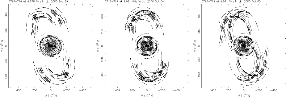
Figure 1: $(u,v)$ coverage of 0716+714 at September 29 (left), October 4 (middle), October 5 (right). The individual coverage are nearly identical, which allows a reliable comparison of the obtained maps.

An array of 12 antennas consisting of the 10 stations of NRAO’s VLBA, the 100 m radio telescope of the Max-Planck-Institut für Radioastronomie in Effelsberg (Germany), and the 8 m HALCA antenna of the VSOP was used to follow the short-term variability of 0716+714 at 5 GHz within one week. The source was observed at 5 GHz during three epochs, namely September 29 (project code: V053 A2), October 4 (V053 A4), and October 5 2000 (V053 A5). We note that a total intensity VSOP image of 0716+714 from these experiments was used already in another publication, where we study the long-term jet kinematics of the sources (Bach et al. 2005, hereafter B05). Each of the three 16 h VSOP observations resulted in dense and nearly identical ($u,v$)-coverages, which are shown in Fig. 1. The details of the observations are summarised in Table 1. The sources 0836+710 and 0615+820 were used as calibrators for the ground array to check the stability of the amplitude calibration between the epochs and to calibrate the polarization data. The calibrators were not observed by the HALCA antenna, because it is not possible to steer HALCA to different source positions during one observation.

Table 1: Observing log. The total integration time, mutual observing time with HALCA, total flux density, the uniform weighted beam size, and the residual noise are given for each epoch and each source.

Epoch	Source	Int.	HALCA	$S_{\rm tot}$	Beam, P.A.	$S_{\rm rms}$
		[h]	[h]	[Jy]	[${\rm mas\times mas}$], [∘]	[mJy]
Sep. 29	0716+714	7.67	2.75	0.55	$0.58\times 0.27$, $-80$	0.492
		7.67	0.00	0.58	$0.95\times 0.78$, $-26$	0.034
	0836+710	1.17	0.00	2.23	$1.10\times 0.88$, $-10$	0.193
	0615+820	1.17	0.00	0.74	$0.90\times 0.78$, $-42$	0.191
Oct. 4	0716+714b	7.72	4.59	0.52	$0.58\times 0.23$, $-79$	0.513
		7.72	0.00	0.55	$0.92\times 0.77$, $-25$	0.041
	0836+710	1.20	0.00	2.28	$0.99\times 0.83$, $-46$	0.168
	0615+820	1.19	0.00	0.75	$0.84\times 0.82$, $-47$	0.173
Oct. 5	0716+714b	7.92	5.47	0.52	$0.58\times 0.24$, $-71$	0.580
		7.92	0.00	0.56	$0.85\times 0.81$, $-28$	0.038
	0836+710	1.21	0.00	2.27	$0.96\times 0.81$, $-74$	0.175
	0615+820	1.23	0.00	0.76	$0.93\times 0.76$, $-55$	0.171

The 100 m RT at Effelsberg not only participated as a VLBI antenna, but also was used to monitor the flux density and polarization variability of all programme sources. These flux density measurements were made in gaps between VLBI scans using pointing cross-scans in azimuth and elevation. From this and the flux and polarization measurements of primary calibrators (3C 286, 3C 48 and 3C 295) before and after the VLBI experiments, the orientation of the polarization E-vector (EVPA, Electric Vector Position Angle) was also obtained (see Sect. 2.2 for details).

The data were recorded in VLBA format with two 16 MHz baseband channels per circular polarization in two-bit sampling, resulting in a recording rate of 128 Mbps at the ground array stations. The HALCA antenna observed only LCP and the data was recorded at several tracking stations (typically 3 per epoch). The correlation was done at the VLBA correlator in Socorro, NM.

Although HALCA is only able to observe in left circular polarization (LCP), VLBI polarimetry becomes possible, if enough other stations of the remaining VLBI array measure both circular polarizations. It is possible to cross-correlate LCP from HALCA with RCP from the ground array stations and thus obtain the cross-polarized correlations on the space baselines. Normally one needs both cross polarizations, $RL$ and $LR$, to image the linear polarization of a source; but using a complex $Q+iU$ image, it is possible to include antennas with only a single cross polarization (e.g., AIPS Memo 79, 1992, W.D. Cotton). Further details about polarization observations using HALCA are given in, e.g., Gabuzda (1999), Kemball et al. (2000), and Gabuzda & Gómez (2001).

The post-correlation analysis was done using NRAO’s Astronomical Image Processing System (Aips). After loading the data into Aips, the standard amplitude and phase calibrations were performed. Since HALCA does not provide pulse calibration information, a manual phase calibration was done to remove offsets between the two intermediate frequency channels (IFs).

At this point the data were exported as $(u,v)$-FITS files (task FITTP) from Aips to Difmap (Shepherd 1994), where the imaging, phase, and amplitude calibration was done, using the CLEAN (Högbom 1974) and SELFCAL procedures. Because of the small diameter of the HALCA antenna, the data from the ground array stations yield a much better signal-to-noise ratio (Fig. 2). Therefore, we first imaged the ground array data alone to obtain a good initial Stokes $I$ image. After this, we included the HALCA antenna in the imaging and self-calibration process, using a strong Gaussian taper (10 % at 450 M $\lambda$) during the first iterations and subsequently decreasing the taper. All images were obtained using uniform weighting. For the ground array images the gridding weights were scaled by the amplitude errors raised to the power $-2$, which favours high quality data with small errors, and for the VSOP images equal weights were applied to achieve highest possible angular resolution. The amplitude errors were derived by the scattering of the data when we averaged the data sampled at 4-second intervals to 60-second intervals.

The self-calibration was done in total intensity in steps of several phase-calibrations followed by careful amplitude calibration. During the iteration process, the solution interval of the amplitude self-calibration was shortened from intervals as long as the whole observational time (in the initial imaging steps) down to minutes at the end of the imaging process. Finally the self-calibrated data were reimported into Aips (using task FITLD), where the calibration of the leakage terms (D-terms) and the polarization imaging was done.

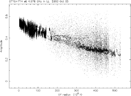
Figure 2: Amplitude vs. $(u,v)$-distance of 0716+714 (Oct. 5). Clearly visible is the higher noise at the HALCA baselines at large $(u,v)$-distances. The dotted line (marginally visible in the centre of the HALCA data) represents the final clean model.

2.1.1 Feed calibration

Calibration of the instrumental polarization and the leakage terms (D-terms) from the left to the right circular polarization feeds at each antenna was done using the task LPCAL in Aips (for the method see: Leppänen et al. 1995). Therefore the total-intensity model produced with IMAGR was split into sub-models using the task CCEDT. The model was separated into three to four sub-models that should represent a small number of “isolated components”, with clearly defined individual polarization properties, suitable for determining the instrumental cross-polarization with LPCAL. This was done in several steps and with different sub-models, to ensure that the D-terms do not depend critically on the choice of the different source and sub-models.

The LPCAL algorithm is robust against different source structures, nevertheless one should prefer core-dominated sources for the calibration. All sources in our observations meet this criterion. The VLBA antennas and Effelsberg exhibit D-term values between 0.5 % and 2 %. For HALCA we derived about $4$ %, similar to what was found by previous observations (e.g., Gabuzda 1999). A number of feed solutions were calculated by using slightly different source models and/or different calibrator sources (0816+710 and 0615+820). The RMS differences between these D-terms are typical smaller than 0.3 % for the ground array stations and reach $\sim 0.5$ % for the HALCA satellite. The D-terms of HALCA could only be checked with different source models of 0716+714, since the calibrators were not observed by the satellite. Plots of the real versus imaginary cross-hand polarization data indicated that a satisfactory D-term solution was obtained. This was also verified in plots of the real and imaginary cross-hand data versus $(u,v)$ parallactic angle. After applying the D-term solution, the variations in the visibility amplitudes with parallactic angle were removed. In Fig. 3 we illustrate this, showing some visibilities before and after application of the D-term calibration.

To estimate how the D-term variations affect the source polarization images, fractional polarization maps with different feed calibration tables were made and then subtracted. The residual amount of fractional polarization in the subtracted images can be used to measure the uncertainty introduced by the different calibrations. This yields an accuracy of $\Delta P/P=0.1$ % in fractional polarization for the VLBI core of 0716+714 and $\Delta P/P=1.2$ % for the weaker jet. The effect of different D-terms on the accuracy of the EVPA was measured in a similar way. Here we obtained an uncertainty of the orientation on the E-vector of $\Delta{\rm EVPA}=0.3^{\circ}$ for the core and $\Delta{\rm EVPA}=2.0^{\circ}$ for the jet.

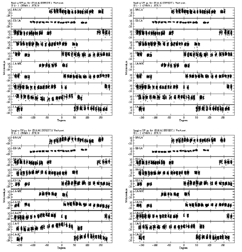
Figure 3: An example for the tests made to check the reliability of the D-term solutions: the panels show the real (top) and imaginary part (bottom) of the Stokes $U$ data on all ground array baselines to Los Alamos plotted versus the parallactic angle (Sep. 29). Left panels: Before application of D-term calibration. Right panels: After the D-term calibration was applied. The calibration successfully removes the systematic variation of the amplitude with parallactic angle.

2.1.2 Polarization imaging

The usual imaging technique for linear polarization is to form $Q$ and $U$ values from the observed $RL$ and $LR$ correlations and separately image and deconvolve the $Q$ and $U$ images. The Aips task COMB can be used to combine the $Q$ and $U$ images to obtain a linear polarization intensity map ($I_{\rm P}=\sqrt{Q^{2}+U^{2}}$) and a map that represents the electric vector polarization angle ($EVPA=\chi=0.5\,\arctan{\frac{U}{Q}}$). But this is only possible in observations where both cross-polarized correlations, $RL$ and $LR$, are available for each interferometer baseline.

Since the HALCA antenna observed only in LCP, only one of the two cross polarized correlations is available for the space-baselines. Nevertheless, it is still possible to form a linear polarization image: in this case complex imaging with a complex deconvolution of $Q+iU$ has to be applied. The Aips software package also offers these tasks. We used the procedure CXPOLN to build the complex image and beam, along with the task CXCLN, which does the complex cleaning and which provides the cleaned $Q$ and $U$ images. These images were then combined with COMB in the usual way to obtain linear polarization intensity and polarization angle images.

2.1.3 EVPA calibration

For the EVPA calibration we used Effelsberg measurements of the quasar 0836+710, orienting its E-vector to ${\rm P.A.}=106.3\,^{\circ}$, previously determined from measurements relative to the primary calibrator 3C 286. We further assumed that between the angular scales covered by the Effelsberg beam and the VLBI scale, there is no dominant polarized component that could affect the EVPA calibration of the VLBI data. The existing VLA maps of 0836+710 support this assumption, as does the comparison of the total intensity and linear polarization measurements at Effelsberg (Tables 3 & 6) with the flux density seen with the VLBA (Table 1 & 2).

Table 2: Comparison of the polarization properties of 0836+710 on single-dish ($P_{\rm Eff}$ and $\chi_{\rm Eff}$) and VLBI ($P_{\rm VLBI}$ and $\chi_{\rm VLBI}$) scales. Using the fixed EVPA from Effelsberg, the measured EVPA from VLBI was corrected by $\Delta\chi=\chi_{\rm Eff}-\chi_{\rm VLBI}$. The different value for the correction in the last epoch is due to the choice of a different reference antenna during the calibration.

Epoch	$P_{\rm Eff}$	$\chi_{\rm Eff}$	$P_{\rm VLBI}$	$\chi_{\rm VLBI}$	$\Delta\chi$
	[mJy]	$[^{\circ}]$	[mJy]	$[^{\circ}]$	$[^{\circ}]$
29 Sep	$160\,\pm\,1$	$106.3\,\pm\,0.3$	$131\,\pm\,13$	$125.8\,\pm\,1.2$	$-19.5\,\pm\,1.2$
04 Oct	$160\,\pm\,1$	$106.3\,\pm\,0.3$	$133\,\pm\,13$	$125.6\,\pm\,1.0$	$-19.3\,\pm\,1.0$
05 Oct	$160\,\pm\,1$	$106.3\,\pm\,0.3$	$128\,\pm\,13$	$96.0\,\pm\,1.1$	$10.3\,\pm\,1.1$

2.2 Effelsberg measurements

In gaps between VLBI scans, we measured the flux density and polarization of the program sources and calibrators. The measurements were performed using standard pointing cross-scans with slews in azimuth and elevation. In addition to the VLBI targets, we observed 0951+699 and 3C 286 as additional flux density and polarization calibrators. In Table 3 we summarise the mean flux density (col. 2) for each source, the number of pointing scans (col. 3), the modulation index $m=100\cdot S/\langle S\rangle$, with the mean flux density $\langle S\rangle$ (col. 4), and the reduced chi-square testing the assumption of non-variability.

Table 3: Effelsberg observing log. Shown are the mean flux density, $\langle S\rangle$, the number of scans, $N$, the modulation index, $m$, and the reduced $\chi^{2}_{\rm r}$ from a linear fit (see text for details).

Source	$\langle S\rangle$ [Jy]	$N$	$m$ [%]	$\chi^{2}_{\rm r}$
0615+820 a	$0.773\,\pm\,0.003$	35	0.42	0.08
0716+714 a	$0.747\,\pm\,0.018$	31	2.38	2.25
0836+710 a	$2.500\,\pm\,0.008$	45	0.33	0.05
0951+699	$3.367\,\pm\,0.005$	4	0.14	0.01
3C 286	$7.521\,\pm\,0.074$	11	0.98	0.42
3C 295	$6.593\,\pm\,0.056$	8	0.85	0.31
3C 48	$5.537\,\pm\,0.019$	2	0.34	0.05
$a$: target for VLBI

A detailed description of the Effelsberg data reduction procedures is given in Kraus et al. (2003). In this experiment we used 3C 286, 3C 295, and 3C 48 as the main flux density calibrators ($S_{\rm 3C\,286}=7.50$ Jy, $S_{\rm 3C\,295}=6.59$ Jy and $S_{\rm 3C\,48}=5.63$ Jy) and 0836+710 as a secondary calibrator, which was observed adjacent to each scan on 0716+714. Also 0615+820 was observed regularly as a secondary calibrator and is known to be non-variable at least on time-scales of days (Kraus 1997). The linear polarization measurements were calibrated using 0836+710 and 3C 286, which both have known polarization properties, as well as 0951+699 which is unpolarized, and all only vary over longer time-scales. After calibration, the residual error of the Effelsberg EVPA was $\sim 0.3^{\circ}$.

3 Results

In this section the total intensity and linear polarization maps of 0716+714 from the ground array data and the VSOP data are presented and analysed. The high dynamic range of the ground array data (peak/RMS $\sim 15\,000$) enables us to follow and study the weak jet up to $\sim 12$ mas core separation. The three times higher resolution in the VSOP images allows a detailed study of the core structure and its variability. The results and analysis of the total intensity and polarization measurements with the 100 m RT in Effelsberg are presented in Sect. 3.3. We would like to note that during each of the three VSOP observations, 0716+714 showed only moderate variations in total intensity ($\sim 5$ %, peak to peak during one epoch). A more pronounced variable source would violate the principle of stationarity in aperture synthesis and would lead to a severe degradation of the reconstructed interferometric image. Here, these effects are small and can be neglected.

Imaging simulations performed by Hummel (1987) have shown that intra-day variability during VLBI observations mainly reduces the achievable dynamic range due to residual side lobes in the images without changing the source structure. In these simulations even larger variations ($\sim 80$ %) were considered. Intensity variations of about 5 %, which are present in our observations, are comparable to the usual uncertainties of the $T_{\rm sys}$ measurements ($\sim 5-10$ %), which are used to calibrate the visibility amplitudes. The final images after self-calibration show a nearly constant noise level outside the source structure without any symmetric features indicating that there are no residual side lobes present. Therefore, we can neglect the effects of the IDV on our VLBI maps. The larger variability of the linear polarization (up to $\sim 40$ %) probably degrades the linear polarization images to some extent, but should not severely affect the self-calibration procedure, because the phase and amplitude self-calibration of $LL$, $RR$, $LR$, and $RL$ during the imaging process was done using the total intensity data.

3.1 Ground array data

                                                                                

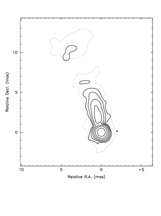
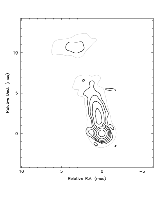
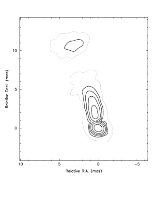
Figure 4: Left panels: Ground array contour maps of Stokes $I$ of 0716+714 with polarization vectors superimposed. The length of the polarization vectors is proportional to the intensity of the linear polarization (1 mas corresponds to 2.5 mJy/beam in $P$). Contours start at 0.13 mJy/beam, increasing in steps of 2. Right panels: Contour maps of the linear polarization. Contours start at 0.25 mJy/beam, increasing in steps of 2. The lowest contour of the total intensity is given by the outer grey line. Time order is from top to bottom: 29 Sep, 4 Oct, and 5 Oct 2000. The beam size, total flux density, and RMS are given in the observing log, Table 1.

The ground array images showing the parsec-scale structure of the jet of 0716+714 are shown in Fig. 4. The panels in the left row show the total intensity contours of 0716+714 with polarization E-vectors superimposed for all three epochs. The right panels of the figure show polarization contour maps. The intensity maps reveal a one-sided core jet structure with a north-oriented jet extending up to $\sim 12$ mas core separation along P.A. $\approx 15^{\circ}$. Between the core and the jet the EVPA is misaligned by $\sim 60^{\circ}$. In the jet and on mas-scales, the electric field vectors are aligned well with the jet axis. Provided that the jet emission is optically thin, which is supported by the high degree of fractional polarization (Fig. 6), the alignment suggests that the magnetic field is oriented perpendicular to the jet axis. The $60^{\circ}$ misalignment of the EVPA of the core can be either explained by Faraday rotation, the fact that the core is optically thick, or by jet bending in the inner most region near the core. High Faraday rotation has been found in many AGN cores (e.g., Zavala & Taylor 2004, 2003 and references therein) with the tendency towards lower rotation measures in BL Lac objects than in quasars, but we are not aware of any rotation measures for the core of 0716+714. However, recent mm-VLBI observations at 43 GHz and 86 GHz show that on the 0.2 mas scale, the jet is strongly curved, oriented along P.A. $\approx 50^{\circ}$ (Fig. 5). This supports the idea that the EVPA orientation follows the bent jet down to the sub-mas scale and that even in the vicinity of the core, the magnetic field is perpendicular to the jet axis.

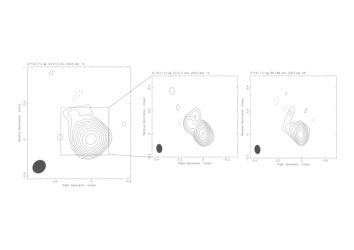
Figure 5: Contour images of 0716+714 at 43 GHz and 86 GHz showing that the jet is bent by about $20^{\circ}$ in the inner 1 mas with respect to the jet at lower resolution. Left: 43 GHz VLBA contour map at a resolution of $166\times 196\,\mu$as at $-43.5^{\circ}$ from March 14, 2003. The peak flux density is 2 Jy/beam and the contours start at 6 mJy increasing in steps of 2. Middle: Super resolved ($76\times 49\,\mu$as at $3.5^{\circ}$) version of the 43 GHz map. Right: 86 GHz map at a resolution of $76\times 49\,\mu$as at $3.5^{\circ}$ from April 28, 2003. Peak flux density is 2.4 Jy/beam and the contours start at 20 mJy.

Inspection of the three 6 cm VLBI images in Fig. 4 reveals no major changes in the total intensity structure between the epochs. Table 1 shows a small and, at this stage, marginal decrease of 5 % in the peak flux from the first to the last two epochs. A more detailed parametrization of the maps, however, is given by Table 4. Here we show the integrated flux densities separately for core and jet.

The measurements were made using the tasks IMSTAT and TVSTAT in Aips, and the errors are derived from the scatter between the individual measurements on slightly different calibrated maps and with different window sizes. The task IMSTAT integrates over a rectangular region that is not necessarily in good agreement with the source structure, whereas TVSTAT integrates over a polygonal region that is specified by the user. We preferred to use IMSTAT and TVSTAT instead of model-fitting Gaussian components to the images, since they also give us more precise measurement of the extended emission.

Attempts to parameterise the total intensity and polarization images with model fitting were focused on the problem that one either needs to use a different number of components to fit $I$ and $P$ or to fix the component position in the $I$ or $P$ images. In both cases one cannot be sure that all of the extended jet emission is adequately represented by the model fit and, more important, if measurements are comparable between the epochs.

Table 4: Summary of the ground VLBI maps.

Epoch		I [mJy]	P [mJy]	$\chi$ [∘]
29 Sep	Core	$520.3\,\pm\,26.9$	$12.1\,\pm\,1.3$	$49.4\,\pm\,4.1$
	Jet	$56.0\,\pm\,\hskip 5.0pt4.7$	$7.4\,\pm\,0.8$	$-10.8\,\pm\,5.6$
04 Oct	Core	$499.3\,\pm\,26.1$	$11.8\,\pm\,1.3$	$40.7\,\pm\,4.0$
	Jet	$54.8\,\pm\,\hskip 5.0pt6.3$	$7.3\,\pm\,0.8$	$-11.2\,\pm\,7.8$
05 Oct	Core	$503.9\,\pm\,25.4$	$6.5\,\pm\,1.1$	$52.7\,\pm\,5.2$
	Jet	$54.7\,\pm\,\hskip 5.0pt6.0$	$7.5\,\pm\,0.8$	$-9.5\,\pm\,7.4$

From Table 4 one can see that the core flux density decreases from 520 mJy to about 500 mJy in the later epochs, whereas the jet flux density stays relatively stable at $\sim 55$ mJy. Using the technique of amplitude self-calibration improves the quality of the VLBI images by applying antenna-based gain corrections to remove residual calibration errors that were not corrected by the a priory amplitude calibration. Provided that the signal-to-noise ratio is sufficiently high, after several iterations the data and the model should converge around an average value set by the a priory amplitude calibration. In these experiment time-dependent station gain corrections of a few percent (typically $\sim 5$ %) were applied. Since the procedure used in all epochs was the same, the relative accuracy of the flux densities after self-calibration should be better than the absolute calibration and can be measured by using the flux of the extended jet emission seen in each experiment. Due to its parsec-scale size, the flux of the integrated jet emission should not be variable on time-scales of days. From Table 4 we obtain 56, 54.8, and 54.7 mJy for the integrated jet flux for each epoch, respectively. Thus, we could attribute this 2.3 % variation between the individual measurements of the extended jet emission to the remaining calibration uncertainty. While the integrated jet flux remained constant at this level, the core flux varied by $\sim 20$ mJy or $\sim 4$ %, a factor of two more than the jet.

In contrast to the marginal variability of the total flux density, strong variability is seen in linear polarization. A visual inspection of the polarization vectors in Fig. 4 indicates that the linear polarization of the core component varies significantly. From the integrated values in Table 4, one can see that there are no changes (within the errors) in the polarized intensity between the first two epochs, but in the last epoch the polarized intensity of the core drops by $\sim$45 %, from $\sim 12.0$ mJy to $\sim 6.5$ mJy, corresponding to a decrease in fractional polarization from $\sim 2.4$ % to $\sim 1.3$ %. As in total intensity, the polarized intensity of the jet shows no variability and stays very constant with a polarized flux of $7.4\pm 0.1$ mJy (or 1.3 % accuracy) at an average degree of polarization of $\sim 13.6$ %. The average EVPA of the jet is also constant at an angle of $-10.5\pm 0.9^{\circ}$, whereas the core EVPA rotates by $\sim 10-13^{\circ}$, from $\sim 50^{\circ}$ to $\sim 40^{\circ}$ and back to $\sim 53^{\circ}$ during the observations.

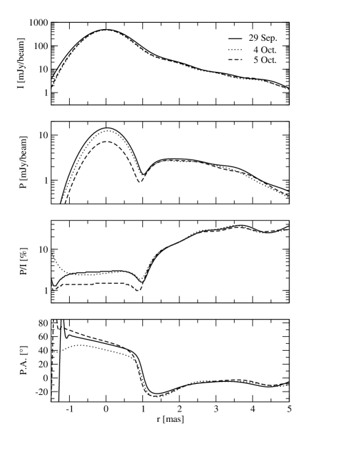
Figure 6: Slices along ${\rm P.A.}=12.5^{\circ}$ through the total intensity, linear polarization intensity, fractional polarization, and EVPA images of the core and the jet of 0716+714.

Figure 6 summarises all these results. It shows profiles of total intensity, linear polarization, degree of polarization, and the orientation of the E-vector plotted versus core separation. To avoid confusion between the different profiles, we did not display the error bars in the plots. The errors of the total intensity and the polarization are dominated by the uncertainties of the amplitude calibration, about 2 %. The error of the EVPA depends on the SNR of the linear polarization and varies between $0.3\,^{\circ}$ for the VLBI core component and about $2\,^{\circ}$ in the bright parts of the jet (see also Sects. 2.1.1 & 2.1.3).

In summary, it seems that between the 3 observations no variation was seen in the jet, neither in intensity nor in polarization. On the other hand, the total flux density of the VLBI core component varied by about $4\pm 2$ % in total intensity and by about a factor of 2 in polarization. The polarization angle of the jet remained constant within $\sim 2^{\circ}$, while the polarization angle of the core varied by $\sim 10^{\circ}$. Therefore all variability appears in the bright and unresolved VLBI core component of 0716+714.

Noticeable are the two peaks of up to 40 % fractional polarization in the jet at $r\approx 2.5$ mas, $r\approx 3.5$ mas, and $r\approx 4.5$ mas distance from the core in Fig. 6. At the same positions, B05 found modelfit components in total intensity, which were used to study the kinematics in the jet. These jet components apparently move superluminally, with speeds of 6.9 $c$ to 8.3 $c$. This provides further evidence that these are real structures in the jet, probably shocks, where we might have a higher density that enhances the total intensity and a more ordered magnetic field that enhances the linear polarization.

3.2 Space VLBI data

Combining the VLBI ground stations with the radio antenna onboard HALCA improves the resolution at 5 GHz by a factor of three (see Table 1). Owing to the small diameter of the HALCA antenna (diameter, $\varnothing=8$ m), the sensitivity on the VLBI baselines to the satellite is relatively low, leading to higher noise on the longest VLBI baselines. The nominal system equivalent flux density (SEFD) of the HALCA antenna is 15300 Jy at 5 GHz (Hirabayashi et al. 2000b) compared to 312 Jy for each VLBA antenna ($\varnothing=25$ m) and 18 Jy for Effelsberg ($\varnothing=100$ m). The uniform weighted $I$ and $P$ images are presented in Fig. 7. To achieve the highest possible resolution, equal weights were applied to all antennas.

In total intensity, the jet extends to core separations of up to 3.5 mas. In comparison to the ground array maps, the jet appears less straight, with bends, followed by back-bends. Although the intensity is weak, the polarization vectors in the jet seem to follow these oscillations. The VLBI core itself completely dominates the weak jet. Due to the 3 times higher resolution with HALCA, it is easier to distinguish between compact emission from the core and extended emission from the mas-jet. The right panel of Fig. 7 shows the polarization contour maps. Owing to their relatively low dynamic range of 70:1, only the VLBI core component is detected at a significant level. Most of the polarized jet emission remains only marginally visible, as indicated by the grey line, which marks the lowest contour of the emission in total intensity. In addition to the core region, a region of slightly enhanced jet polarizations is visible between 1.5 mas to 2 mas from the core. As for the ground array maps, we summarise the integrated flux densities of core and jet in total intensity and polarization in Table 5. Since the marginal detection of linear polarization in the jet prevents reliable measurements, we do not give linear polarization values for the jet in Table 5.

                                                                       

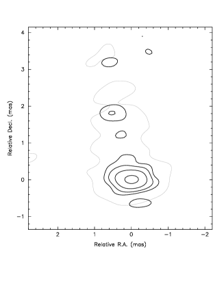
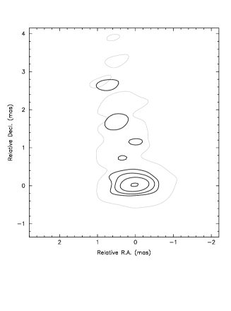
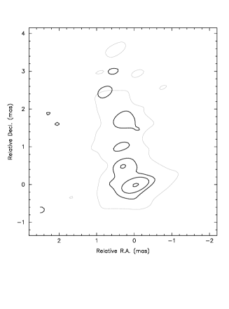
Figure 7: Left panels: VSOP contour maps of Stokes $I$ of 0716+714 with polarization vectors superimposed (1 mas corresponds to 6.7 mJy/beam). Contours start at 1.8 mJy/beam and increasing in steps of 2. Right panels: Contour maps of the linear polarization. Contours start at 1.3 mJy/beam and increasing in steps of 2. The outline of the total intensity is indicated by the outer grey contour. Time order is from top to bottom: 29 Sep, 4 Oct, and 5 Oct 2000. The beam size, total flux density and RMS are given in the observing log, Table 1. Intensity profiles through the core component that better show the variability are given in Fig. 8

In comparison to the ground array data (see Table 4), we measured a core flux density that is $25-35$ % lower, but a jet flux density that was comparable, although the jet is much shorter. This is most likely due to blending effects between core and jet emission, as we could not properly separate both regions using the ground array images. In all three VSOP observations, $\sim 6$ % of the total flux density seen in the ground array maps is missing in the space-VLBI maps. This is reasonable, since the outer jet is partially resolved and therefore much shorter. It is possible to recover the missing flux density by using natural weighting, but this would also decrease the resolution. Since from the ground array images it is already known that the jet flux density is not variable, we can concentrate in the following on the analysis of the core-variability with the highest possible angular resolution.

Table 5: Summary of the flux densities of the VSOP maps (Note that reliable measurements of the jet’s linear polarization were not possible).

Epoch		I [mJy]	P [mJy]	$\chi$ [∘]
Sep 29	Core	$492.5\,\pm\,25.0$	$11.8\,\pm\,2.8$	$49.6\,\pm\,\hskip 5.0pt4.3$
	Jet	$62.4\,\pm\,\hskip 5.0pt4.0$
Oct 4	Core	$465.4\,\pm\,23.6$	$10.8\,\pm\,2.6$	$40.3\,\pm\,4.1$
	Jet	$59.5\,\pm\,\hskip 5.0pt3.7$
Oct 5	Core	$462.4\,\pm\,23.3$	$5.6\,\pm\,1.4$	$54.9\,\pm\,4.5$
	Jet	$60.1\,\pm\,\hskip 5.0pt3.7$

The VSOP images show the same variability behaviour as the ground array images. The total intensity of the core varied at a marginal level of $\sim 6.5$ %. The flux density of the jet emission remained constant at the 4.8 % level. Again, the linearly polarized flux density of the core was highly variable, with an amplitude modulation of a factor 2 between October 4 and 5. The integrated polarization flux densities of the core is comparable to the ground-array images, which suggests that the linear polarized component itself is still compact on the VSOP scales ($\leq 0.25$ mas). We note that 0716+714 was recently detected with VLBI at 230 GHz on transatlantic baselines (Krichbaum et al. 2004). This sets an upper limit to the source size of $\sim 20\,\mu$as, an order of magnitude smaller than the resolution obtained by VSOP.

As in the ground array maps, the EVPA in the core of 0716+714 rotates between the three epochs. Within the measurement errors, the vectors rotated by the same amount as in the ground array images, namely around $-9^{\circ}$ between the first and the second epochs and around $+12^{\circ}$ between the second and the third epochs. The source profile of the VSOP-images is shown in Fig. 8. For the core region, it looks very similar to the profiles from the ground-array images (Fig. 6). The VSOP profiles reveal a small but clearly visible position shift of the linear polarized peak between the epochs. Since these shifts are very small ($<50$ $\mu$as), we are not confident that they are real. Small position shifts could be caused by the motion of the components, which – with regard to the short observing time interval (6 days) and the resulting extreme apparent velocities – does not appear very likely. An alternative and perhaps more realistic interpretation could invoke blending effects between two or more polarized and variable sub-components, located below the angular resolution of this data sets and inside the core region (see also Sect. 4.3).

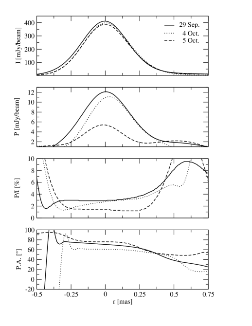
Figure 8: Slices along ${\rm P.A.}=12.5^{\circ}$ through the VSOP images of the core of 0716+714 in total intensity, linear polarization intensity, fractional polarization and EVPA. It is a virtual zoom into the core region of Fig. 6, and $r=0$ marks the same position in both plots.

3.3 Results from total flux density measurements

Table 3 summarises the total flux density measurements, which were taken between VLBI scans with the 100 m radio telescope in Effelsberg. The last two columns of the table give the modulation index $m$ and the reduced $\chi^{2}_{\rm r}$ for testing the variability. Comparison of the modulation indices and $\chi^{2}_{\rm r}$ of 0836+71, 0615+82, and 0716+714 clearly shows that 0716+714 was variable during the observations. The formal $\chi^{2}$-test yields a probability of significant intra-day variability of 99.984 %. The same arguments apply for the polarization. In Table 6 we summarise the linear polarization properties of 0716+714 and the polarization calibrators. The calibrators 0615+82 and 0951+69 are not shown since they are unpolarized.

Table 6: Linear polarization as observed by Effelsberg. $\langle\rangle$ indicate mean values.

Source	$\langle P\rangle$	$\langle P/I\rangle$	$m_{\rm P}$	$\chi^{2}_{\rm r}$	$\langle\chi\rangle$	$\chi^{2}_{\rm r}$
	[mJy]	[%]	[%]		[∘]
0716+71	$19.9\,\pm\,\hskip 3.5pt3.3$	$2.7\,\pm\,0.4$	$9.26$	$15.39$	$18.8\,\pm\,\hskip 3.5pt4.6$	$24.2$
0836+71	$160.0\,\pm\,\hskip 3.5pt1.1$	$6.4\,\pm\,0.1$	$0.00$	$0.05$	$106.3\,\pm\,\hskip 3.5pt0.3$	$0.2$
3C 286	$823.3\,\pm\,12.8$	$11.0\,\pm\,0.3$	$0.78$	$0.27$	$33.0\,\pm\,\hskip 3.5pt0.2$	$0.2$

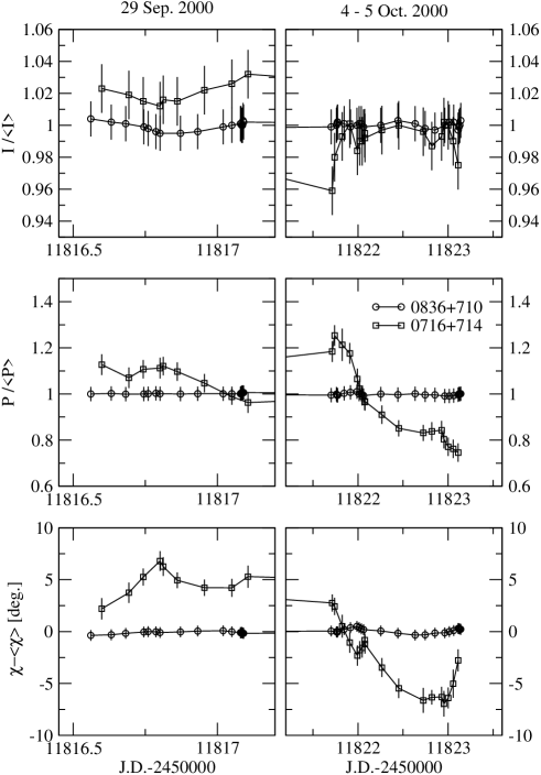
Figure 9: Total intensity (top), linear polarization (middle), and EVPA variations of 0716+714 and the calibrator 0836+710, as measured at Effelsberg at 5 GHz. The left panel shows the data from September 29 and the right panels from October 4 to 5 (note that the time axis between left and right panels differ). For intensity and polarization, we show relative variations, normalised to the mean (average taken over all three days). For the EVPA we plot the absolute difference relative to the mean EVPA. The mean values are given in Table 3 & 6.

Again 0716+714 is the only source that showed significant variability. The total intensity, linear polarization, and EVPA light curves for 0716+714 and 0836+710 are presented in Fig. 9. Since these measurements were made primarily for telescope pointing, the accuracy for flux density measurements is not as high, as it is typically the case for dedicated IDV monitoring observations. We therefore smoothed the light curves, using a three-point running mean, in order to reduce the noise. Figure 9 clearly shows the variability of 0716+714 and the non-variability of its nearby secondary calibrator 0836+710. In 0716+714, up to 5 % variations are seen in total intensity and about 40 % in linear polarization. The polarization angle changed by up to 10 degrees.

4 Discussion

Here we compare the intra-day variability seen in total intensity and linear polarization with the Effelsberg telescope to the variations seen in the VLBI images and discuss then their implications for the origin of the variability (Sect. 4.1 & 4.2) and for the brightness temperature of the VLBI core of 0716+714 (Sect. 4.3). We also discuss possible physical causes for our findings. Using the results of a recent VLBI study of the jet kinematics of 0716+714 (B05), we were able to derive some basic jets parameters, like speed, Doppler-factor, and inclination (Sect. 4.4).

4.1 Origin of variablity

A simple comparison of the average flux density measurements from Effelsberg and the integrated flux densities of the core and the jet region at the three VLBI epochs reveals that all the variablity originates in the VLBI core component (see Table 7). The mean difference between the total flux density in the VLBI maps and the single-dish flux density is ($183.4\pm 3.1$) mJy, corresponding to about 24.5 % less flux density in the VLBI images. This is plausible, since the arcsecond-scale structure of 0716+714 shows two radio-lobes and a surrounding halo-like structure with a diameter of 10 arcsec (Antonucci et al. 1986), which is inside the Effelsberg beam but not seen on VLBI scales. Within the measurement uncertainties, the absolute values of the core variability are similar to those seen at Effelsberg. We observed a decrease of 21 mJy ($\sim 3$ %) with VLBI and 27.5 mJy ($\sim 5$ %) at Effelsberg between epochs one and two and a constant flux density level between epochs two and three. This also confirms our estimate of about 2.3 % for the relative flux density error between the VLBI epochs (Sect. 3.1).

Table 7: The VLBI results in comparison with the single-dish measurements from Effelsberg. The total linear polarization values of the VLBI images were calculated from the vector sum of the core and the jet polarization vectors.

Instrument	Part	I [mJy]	P [mJy]	$\chi$ [∘]
A2: 29 Sep 2000
VLBI	Core	$520.3\,\pm\,26.9$	$12.1\,\pm\,1.3$	$49.4\,\pm\,4.1$
	Jet	$56.0\,\pm\,\hskip 5.0pt4.7$	$7.4\,\pm\,0.8$	$-10.8\,\pm\,5.6$
	Total	$576.3\,\pm\,31.6$	$17.0\,\pm\,2.6$	$27.3\,\pm\,6.0$
Eb		$763.2\,\pm\,\hskip 5.0pt6.9$	$21.4\,\pm\,2.6$	$23.4\,\pm\,2.1$
A4: 4 Oct 2000
VLBI	Core	$499.3\,\pm\,26.1$	$11.8\,\pm\,1.3$	$40.7\,\pm\,4.0$
	Jet	$54.8\,\pm\,\hskip 5.0pt6.3$	$7.3\,\pm\,0.8$	$-11.2\,\pm\,7.8$
	Total	$554.1\,\pm\,32.4$	$17.3\,\pm\,2.7$	$21.3\,\pm\,4.8$
Eb		$735.7\,\pm\,16.2$	$21.6\,\pm\,2.6$	$18.6\,\pm\,2.2$
A5: 5 Oct 2000
VLBI	Core	$503.9\,\pm\,25.4$	$6.5\,\pm\,1.1$	$52.7\,\pm\,5.2$
	Jet	$54.7\,\pm\,\hskip 5.0pt6.0$	$7.5\,\pm\,0.8$	$-9.5\,\pm\,7.4$
	Total	$558.6\,\pm\,31.4$	$12.0\,\pm\,2.3$	$19.1\,\pm\,5.3$
Eb		$740.2\,\pm\,14.6$	$15.7\,\pm\,1.1$	$13.3\,\pm\,2.5$

The variablity of the polarized flux density is anti-correlated with the total intensity variation. The core polarization shows nearly no variation between the first two epochs and a decrease of 5.3 mJy in the VLBI images and 5.9 mJy at Effelsberg between epochs two and three, which corresponds to a 40 % decrease.

Only $4.2\pm 0.3$ mJy of linear polarization are missing in the VLBI maps in comparison to the $\sim 180$ mJy missing in total intensity. This yields an average fractional polarization for the large-scale structure of only 2.3 %, which is small when compared to the $\sim 40$ % linear polarization found with the VLA at 1.4 GHz in the lobe-like structure (Saikia et al. 1987). However, the VLA image shows a variety of EVPA orientations, and the discrepancy is most likely due to in-beam depolarization at Effelsberg, so that polarization vectors at opposite position angles cancel. The missing polarization flux density also causes a difference between the EVPA measured from the VLBI images and at Effelsberg ranging from $2.7^{\circ}$ to $5.8^{\circ}$, but an inspection of the absolute differences between the epochs reveals that the VLBI-core EVPA varied in a similar manner to the EVPA of the Effelsberg data.

Unfortunately, the time sampling of the Effelsberg light curve was not dense enough to measure reliable intra-day variability for most of the time. However, on Oct. 4 the light curve showed a significant decrease in polarization from $(24.5\pm 1.7)$ mJy between $03^{00}$ UT and $07^{00}$ UT to $(20.1\pm 1.1)$ mJy between $14^{00}$ UT and $18^{00}$ UT. At the same time the polarization vector rotated by $(4\pm 2)^{\circ}$. To check whether this polarization IDV is also seen in the VLBI data, the data were split into the corresponding time intervals and imaged separately. The resulting maps show a decrease in the linear polarization in the core from ($13.5\pm 1.4$) mJy to ($9.5\pm 1.0$) mJy (Fig. 10 and Table 8).

Table 8: Linear polarization variability from two time intervals of VLBI data (October 4th) in comparison to the single-dish measurements from Effelsberg.

UT [h]	$P_{\rm Eb}$ [mJy]	$P_{\rm VLBI}$ [mJy]	$\chi_{\rm Eb}$ [∘]	$\chi_{\rm VLBI}$ [∘]
03–07	$24.5\,\pm\,1.7$	$13.5\,\pm\,1.4$	$21.0\,\pm\,2.3$	$40.8\,\pm\,4.2$
14–18	$20.1\,\pm\,1.1$	$9.5\,\pm\,1.0$	$17.2\,\pm\,1.8$	$43.0\,\pm\,5.1$

Although the inaccuracy of the core EVPA measurements in the VLBI images is too large to also confirm a rotation of the EVPA, the very good agreement between the intensity variation from hours to days between the VLBI-core and the single-dish measurements leaves no doubt that the IDV is coming from the VLBI core of 0716+714.

  

Figure 10: Linear polarization contour images of the split Oct. 4 VLBI data with polarization E-vectors superimposed. At a resolution of about 2 mas $\times$ 1 mas at $\sim 85^{\circ}$, the contours start at 0.5 mJy/beam, increasing in steps of 2.

We note that similar variations were previously observed in the IDV sources 0917+624 and 0954+658, where ground-based VLBI observations revealed significant polarization IDV on mas-scales, without showing large variations in the total intensity (Gabuzda et al. 2000b).

4.2 Multiple components

The only moderate variability of the total intensity, the relatively large variation of the polarized flux density, and the relatively small variation of the polarization angle indicate that the variations are caused by the vector sum of the variability of multiple compact and differently polarized sub-components, which are located within the VLBI core region on scales that are smaller than the beam size. The slope of the polarization angle over the core region as seen with the higher resolution from the VSOP data (see Fig. 8) supports the idea that the VLBI core component itself is a composite of several sub-components. Such a multi-component structure is required to explain the polarization IDV by refractive interstellar scintillation (RISS) (e.g. Rickett et al. 1995; Rickett 2001b; Qian et al. 2001), but is also indispensable in models using solely jet intrinsic (e.g. Qian 1993) or mixtures of intrinsic and extrinsic effects (Qian et al. 2002).

If interstellar scintillation is the dominant cause of the variability of the sub-components, their size cannot be much larger than the scattering size of the interstellar medium, which at 5 GHz and towards 0716+714 is believed to be of the order of several ten micro-arcseconds (e.g. Rickett et al. 1995). Under these circumstances, the number of sub-components located within the VLBI-core region (smaller than about 100 $\mu$as, see next section) is limited to a few. The independent and possibly partly quenched scintillation (Rickett 1986) of the sub-components could then explain the variability of the polarization intensity and the variation in the polarization vector. The relative strength of the variability of the polarized flux density ($\sim 40$ %) suggests (i) that at least one of the sub-components is considerably smaller than the scattering size (strong scintillation), and (ii) that the number of independently variable components is not very large, otherwise the time averaged vector sum of the polarization would cancel. Since the polarization angle variations are small ($\leq 15^{\circ}$), we conclude that either (i) the polarization vectors of the sub-components are more or less aligned or (ii) that the more variable sub-component has to be less polarized than the less variable (and most likely more extended) sub-component.

It is tempting to identify the smaller and less polarized sub-component with the optically thick jet-base and the larger and more polarized sub-component with the optically thin inner jet. The fact that the total intensity is less variable than the polarized intensity indicates that the polarized sub-components are considerably smaller than the component(s), which dominate in total intensity. Of course, this simple scenario could change, if a larger number of independently varying sub-components exist or if some sub-components vary in a coherent manner. It is also possible that the variability of the sub-components is not due to scintillation, but is source intrinsic or, more likely, a mixture of both effects.

4.3 Brightness temperature

Assuming that the variability has, at least partly, an intrinsic origin restricts the emitting region to being extremely compact, which then results in very high brightness temperatures exceeding the inverse-Compton limit of $10^{12}$ K (Kellermann & Pauliny-Toth 1969). The short time-scales observed imply linear dimensions of

$$l=\frac{c\,\delta\,\Delta t}{1+z},$$ (1)

where $\delta$ is the Doppler factor. Assuming stationarity and a redshift of 0.3, the size of the emission region responsible for the variability is around $8\cdot 10^{12}$ m or $\sim 55$ A.U., which is slightly larger than our solar system. The brightness temperature for a stationary source is given by

$$T_{\rm b}=3.06\times 10^{8}\ S\ \left(\frac{d_{\rm L}}{\nu\ t\ (1+z)^{2}}\right)^{2}$$ (2)

where $S$ (in Jy) is the flux density, $d_{\rm L}$ (in Mpc) the luminosity distance, $\nu$ (in GHz) the observing frequency, $t$ (in yr) the variability timescale, and $z$ the redshift. The luminosity distance was calculated by adopting an analytical fit by Pen (1999) resulting in $d_{\rm L}=1545.8$ Mpc (see also B05). To calculate the variability time-scale we use:

$$t=\frac{\langle S\rangle}{\Delta S}\ \frac{\Delta t}{(1+z)},$$ (3)

where $\langle S\rangle$ (in Jy) is the mean flux density, $\Delta S$ (in Jy) the standard deviation, and $\Delta t$ (in yr) the duration of the variation (e.g. Wagner et al. 1996). Calculating the corresponding $T_{\rm b}$ of the linear polarization decrease between October 4th and 5th ($\langle S\rangle=9.2$ mJy, $\Delta S=3.8$ mJy, and $\Delta t=24$ h) results in $T^{\prime}_{\rm b}\approx 3.8\times 10^{15}$ K and the decrease during October 4th ($\langle S\rangle=11.5$ mJy, $\Delta S=2.8$ mJy, and $\Delta t=10$ h) yields $T^{\prime}_{\rm b}\approx 9.6\times 10^{15}$ K. Since the observed brightness temperature $T^{\prime}_{\rm b}$ derived from variability is connected to the intrinsic brightness temperature by $T^{\prime}_{\rm b}=T_{\rm b}\cdot\delta^{3}$, a Doppler factor of 14 to 22 is needed to reduce the brightness temperature to the inverse-Compton limit. These calculations usually require a densely sampled light curve to estimate $\langle S\rangle$, $\Delta S$, and $t$. However, considering that, due to the insufficient sampling we, have probably not observed the full amplitude or missed the most rapid variations, the calculated values of $T_{\rm b}$ are underestimates rather than overestimates of the true values.

If instead of the inverse-Compton limit, the equipartition brightness temperature of $5\times 10^{10}$ K to $10^{11}$ K is used (cf. Readhead 1994), a Doppler factor of up to 60 is obtained. However, only a small departure from equipartition, e.g. by a factor of two, would bring the Doppler factor back to 30, which is well within the range of possible Doppler factors derived from our kinematic study (B05).

Gaussian modelfits to the VSOP $(u,v)$-data of the first epoch reveals a flux density of ($0.42\pm 0.06$) Jy and a size of $(0.09\pm 0.02$) mas for the core component. Since the core is not resolved, the size only represents an upper limit. However, this measurement already yields a brightness temperature of $(2.6\pm 0.7)\times 10^{12}$ K and therewith exceeds the inverse-Compton limit. To bring these temperatures down, a Doppler factor of $>4$ is needed. We note that all these values depend on the redshift of 0716+714 which is not yet known. The used value of $z=0.3$ is based on the non-detection of an underlying host galaxy (Wagner et al. 1996), but newer studies already place the limit to $>0.5$ (Sbarufatti et al. 2005) which would increase the observed $T^{\prime}_{\rm b}$ by at least a factor of three. A lower limit of the Doppler factor of 2.1 comes from synchrotron self-Compton (SSC) models (Ghisellini et al. 1993).

The VSOP 5 GHz AGN survey (Hirabayashi et al. 2000a), which contains nearly all extra-galactic flat-spectrum radio sources brighter than 1 Jy and at galactic latitude $\geq 10\,^{\circ}$ ($\sim 300$ sources), has shown that about 50 % of these types of sources have brightness temperatures of $T_{\rm b}>10^{12}$ K, and about 20 % even have $T_{\rm b}>10^{13}$ K (Scott et al. 2004; Horiuchi et al. 2004). The VSOP observations of a sub-sample ($\sim 30$ sources) of the Pearson-Readhead sample (Pearson & Readhead 1988) revealed a significant correlation between the IDV activity and the brightness temperature (Tingay et al. 2001). The authors find that sources showing rapid IDV have higher brightness temperatures than weakly variable or non-IDV sources. Therefore, independent of the physical model for the variability, relativistic beaming seems to play a role.

4.4 Jet inclination and Lorentz factor

Simulations of relativistic hydrodynamic jets show that shocks are likely to occur in highly supersonic flows. Those provide a natural way to locally enhance the magnetic field and relativistic electron density, producing knots of emission such as seen in VLBI images (e.g., Goméz et al. 1997, and references therein). Assuming that the knots in the jet are shocks travelling down the jet, we can use the observed degree of polarization of such a jet component to set limits on the angle to the line of sight and on the jet Lorentz factor (Cawthorne & Wardle 1988). The shock model used here is based on the scenario that Hughes et al. (1985) used to describe the polarization variability in BL Lac. In that model, a propagating shock compresses the magnetic field of the jet so that the initially random field is ordered in a plane transverse to the jet axis. With this we can constrain the amount of compression, defined as a unit length compressed to a length $k$, and the angle between the line of sight and the shock plane in the frame of the jet ($\epsilon$) using the measured degree of polarization ($m$) in the jet. If we assume that the shock travels with the same velocity as the emitting material, we can also relate $k$ and $\epsilon$ to the apparent speed of the jet and constrain the inclination of the jet, $\theta$, and the jet Lorentz factor, $\gamma$ (Cawthorne & Wardle 1988).

A modelfit to the linear polarization image with JMFIT in Aips reveals that the peak of the linear polarization in the jet corresponds to component C7 (B05), which moves with a speed of $(6.9\pm 0.2)\,c$ assuming $z=0.3$. Integrating the flux density in the total intensity and in the polarization image over a region of 1.5 times the beam width around the component centre ($r=2.7\pm 0.2$ mas) yields a fractional polarization, $m$, of about $(24\pm 4)$ %. For a spectrum of $\alpha_{\rm 5/15\,GHz}=-0.7$ (B05) and therewith $s\approx 2.5$, the nominal degree of polarization of synchrotron emission in a uniform magnetic field is $m_{0}\approx 0.72$.

We would like to distinguish two cases. First, if the jet is oriented at the viewing angle that maximizes the apparent superluminal motion, then $\epsilon=0$ and $k$ gives an upper limit on the amount of compression. We find $k_{\rm min}=0.71\pm 0.04$. Second, if we assume a maximum of compression ($k\ll 1$), then $\epsilon$ corresponds to the maximum angle between the shock plane and the line of sight, which yields $\epsilon_{\rm max}=\pm 45\pm 4^{\circ}$.

In the first case, the measured apparent speed of $(6.9\pm 0.2)\,c$ of component C7 yields a jet Lorentz factor of $\sim 7$ and an angle to the line of sight of $\sim 8^{\circ}$, which would not agree with the results (B05), where a minimum Lorentz factor of $11.6$ and $\theta_{\rm max}=4.9\,^{\circ}$ was found. The second case ($k\ll 1$ and $\epsilon=\pm 45^{\circ}$) yields $\gamma\approx 10$ and $\theta\approx 2.5^{\circ}$ or $14^{\circ}$ (depending on the sign of $\epsilon$), but the larger viewing angle can almost certainly be excluded from the kinematics (B05). From this the second case seems more likely, and the derived jet parameters show the same trend as the parameters ($\gamma>16$ and $\theta<2^{\circ}$) derived by B05. The shock scenario also favours the small-angle solution, where we have higher jet Lorentz factors and smaller viewing angles than those derived by maximization of $\beta_{\rm app}=\frac{\beta\sin\theta}{1-\beta\cos\theta}$. The corresponding Doppler factor is about 17 for $\gamma\approx 10$ and $\theta\approx 2.5^{\circ}$.

5 Conclusions

In order to search for the origin of the rapid IDV in 0716+714, a multi-epoch VSOP experiment was performed in September and October 2000. The ground array and the VSOP images show a bright core and a jet oriented to the north. The linear polarization images indicate that the jet magnetic field is perpendicular to the jet axis. Compared to the jet axis, the electric vector position angle in the core is misaligned by around 60 ^∘. This is explained either by opacity effects in the core region or by a curved jet. Jet curvature is supported by recent high resolution 3 mm VLBI observations that show the inner jet structure ($r<0.1$ mas) at a similar position angle as the EVPA in the core at 6 cm wavelength. A misalignment between the parsec-scale and the kiloparsec-scale structure is typical of BL Lacs (Pearson & Readhead 1988; Wehrle et al. 1992) and is also seen in 0716+714 (VLA images can be found in Antonucci et al. 1986; Gabuzda et al. 2000a; Bach et al., in prep.). The new VLBI observations suggest that the jet bending continues down to sub-parsec-scales. Possible explanations for such a misalignment are a helical jet, which is oriented towards us (Conway & Murphy 1993), possibly due to Kelvin-Helmholtz instabilities (e.g., Hardee 1986, 1981) or to being driven by precession (B05; Nesci et al. 2005), or due to interaction with the surrounding medium.

Simultaneous flux-density measurements with the 100 m Effelsberg telescope during the VSOP observations revealed variability in total intensity ($\sim 5$ %) and in linear polarization (up to $\sim 40$ %) accompanied by a rotation of the polarization angle by up to $15\,^{\circ}$. The analysis of the VLBI data shows that in 0716+714 the intra-day variability is associated to the VLBI-core region and not to the milli-arcsecond jet. Both the ground array and the VSOP maps show a similar decrease of the flux densities in total intensity and linear polarization of the core component, which is in good agreement with the variations in the total flux density and polarization seen with the Effelsberg 100 m radio-telescope. In this, 0716+714 displays a behaviour that is similar to what was previously observed in the IDV sources 0917+624 and 0954+658, where components in or near the VLBI core region were also made responsible for the IDV (Gabuzda et al. 2000b). Over the time interval of our VSOP observations, no rapid variability in the jet was observed and we cannot confirm the variability outside the core and in the jet found by Gabuzda et al. (2000a).

The simultaneous variation of the polarization angle with the polarized intensity in the core suggests that the variations might be the result of the sum of the polarization of more than one compact sub-component on scales smaller than the beam size. Assuming that these variations are intrinsic to the source, we derived brightness temperatures of $\sim 3\times 10^{15}$ K to $\sim 10^{16}$ K. Doppler factors of $>20$ are needed to bring these values down to the inverse-Compton limit. These numbers agree with the observed speeds in the jet if the angle to the line of sight is very small ($\theta<2^{\circ}$), as already proposed by B05. Because of the unknown redshift, the derived speeds and brightness temperatures represent only lower limits.

However, interstellar scintillation effects could also explain the IDV seen in the VLBI core, if the core region consists of several compact and polarized sub-components, with sizes of a few ten micro-arcseconds. To explain the observed polarization variations, the sub-components must scintillate independently in a different manner, which means that they must have slightly different intrinsic sizes and intrinsic polarizations (i.e. Rickett 2001b, a).

Independent of whether the interpretation of the IDV seen in the VLBI core is source intrinsic or extrinsic, the space-VLBI limit to the core size gives a robust lower limit to the brightness temperature of $\geq 2\times 10^{12}$ K and therewith exceeds the inverse-Compton limit. This implies a lower limit to the Doppler factor of about $\geq 4$ and, independent of the model we use to explain the variability, relativistic beaming seems to play a role. Unfortunately, the possible sub-components inside the core region cannot be observed directly. Future multi-frequency polarization VLBI observations, including simultaneous observations at higher frequencies, should help distinguishing which fraction of the IDV is due to source intrinsic variations and which is caused by the interstellar medium.

To explain the enhanced degree of polarization in the superluminal jet, we applied a simple shock model developed by Cawthorne & Wardle (1988) to our observations and found reasonable values for the jet Lorentz factor and the viewing angle. This supports the idea that the knots of bright emission in the jet are shocks travelling down the jet (Marscher & Gear 1985).