The importance of tides for the Local Group dwarf spheroidals

Abstract

There are two main tidal effects which can act on the Local Group dwarf spheroidals (dSphs): tidal stripping and tidal shocking. Using N-body simulations, we show that tidal stripping always leads to flat or rising projected velocity dispersions beyond a critical radius; it is $\sim 5$ times more likely, when averaging over all possible projection angles, that the cylindrically averaged projected dispersion will rise, rather than be flat. In contrast, the Local Group dSphs, as a class, show flat or falling projected velocity dispersions interior to $\sim 1$ kpc. This argues for tidal stripping being unimportant interior to $\sim 1$ kpc for most of the Local Group dSphs observed so far. We show that tidal shocking may still be important, however, even when tidal stripping is not. This could explain the observed correlation for the Local Group dSphs between central surface brightness and distance from the nearest large galaxy.

These results have important implications for the formation of the dSphs and for cosmology. As a result of the existence of cold stars at large radii in several dSphs, a tidal origin for the formation of these Local Group dSphs (in which they contain no dark matter) is strongly disfavoured. In the cosmological context, a naive solution to the missing satellites problem is to allow only the most massive substructure dark matter halos around the Milky Way to form stars. It is possible for dSphs to reside within these halos ($\sim 10^{10}$M_⊙) and have their velocity dispersions lowered through the action of tidal shocks, but only if they have a central density core in their dark matter, rather than a cusp. A central density cusp persists even after unrealistically extreme tidal shocking and leads to central velocity dispersions which are too high to be consistent with data from the Local Group dSphs. dSphs can reside within cuspy dark matter halos if their halos are less massive ($\sim 10^{9}$M_⊙) and therefore have smaller central velocity dispersions initially.

1 Introduction

The Local Group of galaxies provides a unique test-bed for galaxy formation models and cosmology. The abundance, spatial distribution and internal mass distribution, of satellites within the Local Group can provide sensitive tests of cosmological predictions (see e.g. Moore et al. 1999, Klypin et al. 1999, Kravtsov et al. 2004, Mayer et al. 2001a and Mayer et al. 2001b). However, central to such studies is an understanding of what the Local Group satellite galaxies are. Observationally, they are usually split into three types: dSph galaxies, which typically have old stellar populations, are spheroidal in morphology, lie close to their host galaxyand are devoid of HI gas; dIrr galaxies, which have younger stellar populations, irregular morphology, lie further away from their host galaxy and contain significant HI gas; and the transition galaxies, which are in between the dSph and dIrr types (Mateo, 1998).

Since the dSph galaxies lie, in general, closer to their host galaxy (there are notable exceptions - see e.g. Grebel et al. 2003) it has often been argued that the tidal field of the host galaxy has an important role to play in the formation and evolution of these galaxies. Mayer et al. (2001a) and Mayer et al. (2001b) have suggested that all of the Local Group satellite galaxies started out looking more like the dIrrs, the dSphs then forming through tidal transformations. Kuhn & Miller (1989) and Kroupa (1997) have argued that the dSphs might have formed in the tidal tail of a previous major merger; in their model, dSphs contain no dark matter and are nearly unbound. Stoehr et al. (2002) have argued that the dSphs inhabit the most massive substructure dark matter halos, of mass $\sim 10^{10}$M_⊙, predicted by cosmological N-body simulations (see e.g. Klypin et al. 1999 and Moore et al. 1999); in such a scenario, tides are unlikely to have significantly altered the visible distribution of stars in these galaxies.

Figure 1: Surface brightness profiles (left) and projected velocity dispersions (right) for three Local Group dSphs observed with good stellar kinematics. Data taken from Wilkinson et al. (2004), Kleyna et al. (2004), Irwin & Hatzidimitriou (1995) and Palma et al. (2003); but see also Martínez-Delgado et al. (2001) for deeper surface brightness data for UMi. Notice the similarities between each of the dSphs: the surface brightness profiles are roughly exponential, while the projected velocity dispersions are approximately flat with a sharp fall-off at large radii ($\sim 1$ kpc).

In this paper we compare a suite of N-body simulations of dSph galaxies orbiting in a tidal field, with the latest data from the Local Group dSphs (see Figure 1). In this way, we can constrain the importance of tidal effects for these galaxies and break the degeneracies between the above formation scenarios.

The effects of tides on the Local Group dSphs has been investigated extensively in the literature, both dynamically (Aguilar & White 1986, Oh et al. 1995, Piatek & Pryor 1995, Hayashi et al. 2003, Kazantzidis et al. 2004 and Mashchenko et al. 2005), and within a cosmological framework (Kravtsov et al., 2004). This present work complements that of previous authors. Like Hayashi et al. (2003) and Kazantzidis et al. (2004), we perform simulations which are not fully cosmologically consistent, but which have the advantage that the simulated satellites have very high resolution. Unlike these previous authors, however, our dSph galaxies contain both stars and dark matter. This allows us to compare our results more easily with the observational data from the Local Group dSphs.

We consider three possible scenarios for the tidal evolution of the Local Group dSphs. In the first (model A), we revisit the hypothesis that the Local Group dSphs contain no dark matter and that their high velocity dispersions arise instead from the action of tides. In the second scenario (models B and C), we investigate the hypothesis that the dSphs are dark matter dominated, but that their outer regions have been shaped by tidal effects. In this case we ask whether tides could directly cause the drop in projected velocity dispersion in the outer regions of the dSphs, recently observed by Wilkinson et al. (2004); and see also Figure 1. In the third scenario (model D), we investigate a scenario where dSphs were much more massive in the past. In this case, tidal shocks cause their central density and velocity dispersions to fall significantly over a Hubble time, becoming consistent with current data at the present epoch. It is important to state explicitly here that we do not wish to model any one specific Local Group dSph, which would require an extensive search through parameter space and probably not be relevant when taken out of a cosmological context. Rather, we wish to investigate the generic effects of tides and how they reshape a dSph.

This paper is organised as follows: in section 2, we briefly outline some key analytic results for tidal stripping and tidal shocking - the two dominant tidal effects which act on a satellite orbiting in a host galaxy potential. The analytic results and definitions therein will be referred to throughout this paper and are useful in both understanding and testing the simulation results. In section 3, we describe our numerical method for setting up the initial conditions and integrating the orbit of the satellite in the fixed potential of the Milky Way. In section 4, we present the results from a set of representative N-body simulations simulations. We demonstrate that tidal stripping will always lead to a flat or rising projected velocity dispersion. In section 5 we discuss our results in the context of cosmology; we place mass limits on the Local Group dSphs. Finally, in section 6 we present our conclusions.

2 Theoretical background

Model	$\rho_{*}$	$\rho_{DM}$	$N_{*}$	$\xi_{*}$(kpc)	$N_{DM}$	$\xi_{DM}$(kpc)	Orbit	Time(Gyrs)	$\gamma$
A	P: 5, 0.23	None	$10^{5}$	$0.01$	-	-	9 kpc,84 kpc,-34.7o	10.43	0.0011
B	P: 0.072, 0.23	P: 14, 0.5	$10^{5}$	$0.01$	$10^{6}$	$0.01$	23 kpc,85 kpc,-34.7o	4.5	0.00014
C	SP: 0.072, 0.1, 0	SP: 90, 1.956, 1	$10^{5}$	$0.01$	$10^{6}$	$0.01$	23 kpc,85 kpc,-34.7o	4.5	0.15
D	SP: 0.072, 0.1, 0	SP: $10^{3}$, 1.956, 1	$10^{5}$	$0.01$	$10^{6}$	$0.01$	6.5 kpc,80 kpc,7.25o	8.85	0.83

Table 1: Simulation initial conditions for models A-D. The columns from left to right show the model (labelled by a letter in order of discussion), the stellar density profile, $\rho_{*}$, the dark matter density profile, $\rho_{DM}$, the number of stars, $N_{*}$, the force softening for the stars, $\xi_{*}$, the number of dark matter particles, $N_{DM}$, the force softening for the dark matter, $\xi_{DM}$, the dwarf galaxy orbit, the output time in Gyrs at which we show the results from the model and the strength of tidal shocks, $\gamma$ (see section 2.2). The density profiles are either (P)lummer with parameters: mass ($10^{7}$M_⊙), scale length (kpc) or (S)plit (P)ower law with parameters: mass ($10^{7}$M_⊙), scale length (kpc) and central log slope, $\alpha$ (see equations 11 and 13 for more details). The orbit for the dwarf galaxy is given by its pericentre, apocentre and inclination angle to the Milky Way disc.

A satellite in orbit around a host galaxy will experience two main tidal effects which will reshape the stellar and dark matter distributions: tidal stripping and tidal shocking. Since both of the mechanisms will be referred to many times throughout this paper, it is instructive to briefly outline the salient properties of each in this section.

2.1 Tidal stripping

We discuss the theory of tidal stripping in much more detail in a companion paper, Read et al. (2005). Here we briefly summarise the main results of that work. Tidal stripping refers to the capture of stars by a host galaxy from a satellite galaxy beyond a critical radius: the tidal radius, $r_{t}$. In general, the tidal radius depends upon four factors: the potential of the host galaxy, the potential of the satellite, the orbit of the satellite and, which is new to the calculation presented in Read et al. (2005), the orbit of the star within the satellite. In Read et al. (2005), we demonstrate that this last point is critical and suggest using three tidal radii to cover the range of orbits of stars within the satellite. In this way we show explicitly that prograde star orbits will be more easily stripped than radial orbits; while radial orbits are more easily stripped than retrograde ones.

In general, these three tidal radii must be calculated numerically as outlined in Read et al. (2005). We will use these more accurate numerical calculations in the presentation of tidal radii later on in this paper. However, for the special case of point mass potentials, $r_{t}$ reduces to the following simple form:

$$r_{t}\simeq x_{p}\left(\frac{M_{s}}{M_{g}}\right)^{1/3}\left(\frac{1}{1+e}\right)^{1/3}\left(\frac{\sqrt{\alpha^{2}+1+\frac{2}{1+e}}-\alpha}{1+\frac{2}{1+e}}\right)^{2/3}$$ (1)

where $x_{p}$ and $e$ are the pericentre and eccentricity of the satellite’s orbit, $M_{s}$ is the total mass of the satellite, $M_{g}$ is the mass of the host galaxy and $\alpha=-1,0,1$ parameterises the orbit of the star within the satellite. From equation 1, we can see that stars on prograde orbits ($\alpha=1$) are more easily stripped than those on radial orbits ($\alpha=0$), which are more easily stripped than those on retrograde orbits ($\alpha=-1$). Notice that $\alpha=0$ recovers the standard King (1962) tidal radius. Other analytic solutions also exist for power-law and a restricted class of split power-law density profiles (Read et al., 2005).

Over long times, orbital transformations cause a convergence of these three tidal radii on the prograde stripping radius and leads to the onset of tangential anisotropy beyond this point.

A final key result from Read et al. (2005) is that the standard intuition that the tidal radius depends only (within a factor) on the densities of the host galaxy and satellite galaxy is only valid for stars within the satellite which are on radial orbits. For general star orbits, their stripping radius will depend upon the mass distribution within the satellite and not just the enclosed mass.

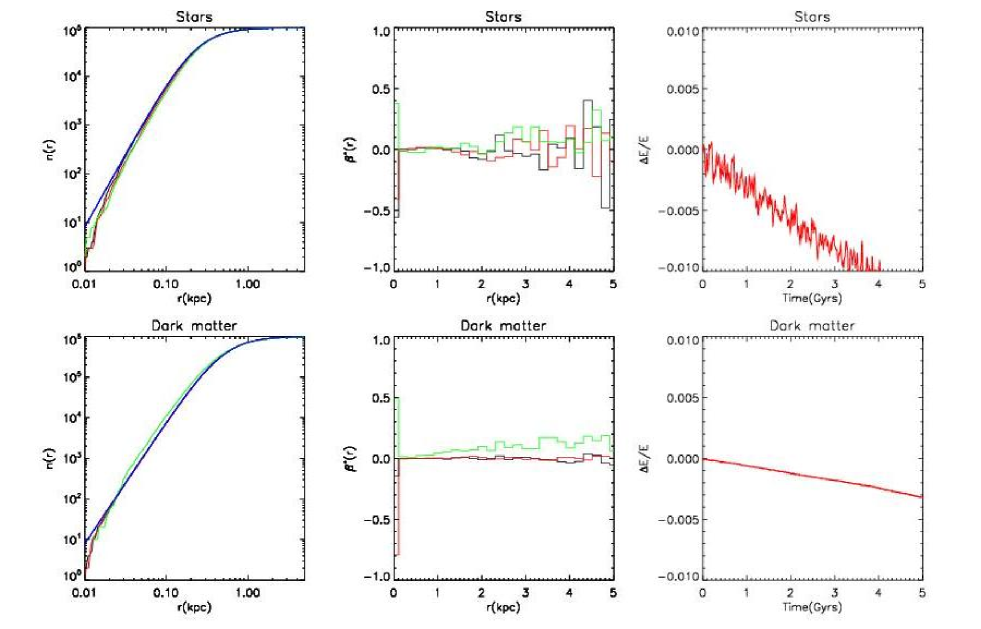
Figure 2: Equilibrium tests for model A: The upper panels are for the stars, while the lower panels are for the dark matter. The left panels show the cumulative mass profile, the middle panels show the velocity anisotropy and the right panels show the fractional change in energy as a function of time. The blue lines are for the analytic initial conditions, the black lines are for the simulated initial conditions with $10^{6}$ dark matter and $10^{5}$ star particles, the red lines are for the simulated initial conditions evolved for 5 Gyrs, while the green lines are for a simulation set up using the Maxwellian approximation (Hernquist, 1993) and evolved for 5 Gyrs.

2.2 Tidal shocking

A second important effect of tides is tidal shocking. Tidal shocks can be caused either as a satellite plunges through the disc of the host galaxy (see e.g. Ostriker et al. 1972) or moves on a highly eccentric orbit through the galactic centre (see e.g. Spitzer 1987). Both scenarios are discussed in detail by Gnedin & Ostriker (1997), Gnedin et al. (1999) and Gnedin et al. (1999).

In the impulsive limit, the mean energy injected into the satellite at the r.m.s. radius, $\overline{r}$, for disc shocks is given by (Gnedin et al., 1999):

$$\overline{\Delta E_{\mathrm{disc}}}=\frac{2g_{m}^{2}\overline{r}^{2}}{3V_{z}^{2}}(1+x^{2})^{-\alpha}$$ (2)

where: $g_{m}$ is the maximal disc force along the $z$ direction (in all of the calculations presented in this paper it is a assumed that the plane of the Milky Way disc lies perpendicular to the $z$-axis); $V_{z}$ is the $z$ component of the satellite velocity at the point it passes through the disc; $x=\omega\tau$ ($\omega$ is the angular velocity of a star within the satellite at $r$; $\tau\sim 2H/V_{z}$ is the typical shock time for a disc of scale height, $H$); and $\alpha$ is the adiabatic correction exponent which is $\sim 5/2$ for fast shocks (Gnedin et al., 1999).

Similarly, the mean energy injected for an eccentric orbit in a spherical system (here an isothermal potential for the host galaxy is assumed) is given by (Gnedin et al., 1999):

$$\overline{\Delta E_{\mathrm{sph}}}=\frac{1}{6}\left(\frac{v_{0}^{2}\pi\overline{r}}{R_{p}V_{p}}\right)^{2}(1+x^{2})^{-\alpha}$$ (3)

where $v_{0}$ is the asymptotic circular speed of test particles at large radii in the host galaxy potential, $R_{p}$ is the pericentric radius, $V_{p}$ is the satellite velocity at $R_{p}$ and $x$ is as above, but the shock time is now given by, $\tau\sim\pi R_{p}/V_{p}$.

We make the somewhat crude assumption that the total energy injected into the satellite due to a single shock at $\overline{r}$ is then given by the sum of the above two terms.

Assuming that the satellite is in virial equilibrium before the tidal shock and that it has an isotropic velocity distribution, the total specific energy of the satellite, $E$, is given by:

$$E=-T\sim\frac{1}{2}\overline{v^{2}(\overline{r})}=\frac{1}{2\rho_{s}(\overline{r})}\int_{\overline{r}}^{\infty}{\rho_{s}(r)\frac{GM_{s}(r)}{r^{2}}}dr$$ (4)

where $T$ is the satellite’s total specific kinetic energy, $\overline{v^{2}(\overline{r})}^{1/2}$ is the velocity dispersion, $\rho_{s}(r)$ and $M_{s}(r)$ are the mass and density profile of the satellite and the right hand side follows from the Jeans equations (Binney & Tremaine, 1987).

We assume that tidal shocks are important for the satellite if the energy injected is comparable to the total energy of the satellite initially. This gives:

$$\gamma=2\left[\frac{\overline{\Delta E_{\mathrm{sph}}}+\overline{\Delta E_{\mathrm{disc}}}}{\overline{v^{2}(\overline{r})}}\right]$$ (5)

where $\gamma$ parameterises the importance of tidal shocks: tidal shocks are important for $\gamma\sim 1$ and unimportant for $\gamma\ll 1$. Notice from equations 2, 3 and 5 that the effectiveness of tidal shocks depends on the mass density of the satellite, the potential of the host galaxy and on the orbit of the satellite. The strength of such shocks is very sensitive to the value of $R_{p}$. For the Milky Way potential employed in this paper, both disc shocks and spherical tidal shocks are negligible for orbits which never come closer than $\sim 20$ kpc.

The value of $\gamma$ for each of the four models presented in this paper (labelled A-D) are given in Table 1. Model D is a case of particular interest. For this model, $\gamma\sim 1$ and so tidal shocks are very important. Yet the tidal radius (as obtained using equation 1) lies at the edge of the light distribution. Thus it is possible that some of the Local Group dSphs could be in a regime where their visible light is strongly affected by tidal shocks but only very weakly perturbed by tidal stripping.

3 The numerical technique

3.1 Setting up the initial conditions

3.1.1 The dSph galaxy

The initial conditions for the dSph galaxy were set up in a similar fashion to Kazantzidis et al. (2004), but for two-component spherical galaxies comprising a dark matter halo and some stars. Since this procedure is non-trivial we briefly outline the major steps involved here:

(i) The particle positions for each component are realised using standard accept/reject techniques with numerically calculated comparison functions and analytic density profiles (Press et al., 1992).

(ii) We use isotropic, spherically symmetric, distribution functions (Binney & Tremaine, 1987). For each separate component, $i$, with density, $\rho_{i}$, in the total relative gravitational potential of all components, $\psi$, the distribution function is given by the Eddington formula:

$$f(\epsilon)=\frac{1}{\sqrt{8}\pi^{2}}\left[\int_{0}^{\epsilon}{\frac{d^{2}\rho_{i}}{d\psi^{2}}\frac{d\psi}{\sqrt{\epsilon-\psi}}+\frac{1}{\sqrt{\epsilon}}\left(\frac{d\rho_{i}}{d\psi}\right)_{\psi=0}}\right]$$ (6)

where $\epsilon$ is the specific energy. Note that, for any choice of $\rho_{i}$ and $\psi$ which are well behaved as $r\rightarrow\infty$, the second term in the brackets in equation 6 vanishes (Binney & Tremaine, 1987).

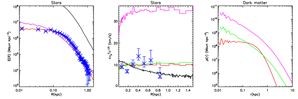
Figure 3: Initial conditions for models A-D. The blue data points are for the Draco dSph galaxy taken from Wilkinson et al. (2004). The black,red,green,purple lines are for models A,B,C,D respectively. Recall that in model A we have no dark matter, hence there is no black line in the right panel plot of the dark matter distribution.

For a general two component system $f(\epsilon)$ must be calculated numerically. In Kazantzidis et al. (2004), where only single component systems (dark matter only) were considered, the term $\frac{d^{2}\rho_{i}}{d\psi^{2}}$ could be calculated analytically. Here, where in general $\psi=\psi_{1}+\psi_{2}+...+\psi_{n}$ for an $n$ component system, this must be calculated numerically. We consider the special case where $\psi_{i}$ and $\rho_{i}$ are known analytically for each component. In this case we can write:

$$\frac{d^{2}\rho_{i}}{d\psi^{2}}=\left(\frac{dr}{d\psi}\right)^{2}\frac{d^{2}\rho_{i}}{dr^{2}}+\frac{dr}{d\psi}\frac{d\rho_{i}}{dr}\frac{d}{dr}\left(\frac{dr}{d\psi}\right)$$ (7)

This means that we can calculate $\frac{d^{2}\rho_{i}}{d\psi^{2}}$ in general analytically for a given value of $r$. This avoids the need for a noisy double numerical differential. However, we do still need to generate a look-up table to solve the inversion for $r(\psi)$. Once this is done, however, we may perform the integral in equation 6 and create a log look-up table for $f(\epsilon)$ over a wide range of $\epsilon$ as in Kazantzidis et al. (2004).

(iii) Once the distribution function, $f(\epsilon)$, is known for each component, we can set up particle velocities using standard accept/reject techniques (Press et al., 1992). We take advantage of the fact that the maximum value of the distribution function at a given point will be given by the maximum value of $\epsilon$; that is for $v=0$ (Kuijken & Dubinski, 1995).

This may seem like an unnecessarily large amount of effort to go to, when simple numerical techniques already exist for setting up multi-component galaxies (Hernquist, 1993). However, as pointed out by Kazantzidis et al. (2004), using approximate methods such as the Maxwellian approximation will lead to a small evolution away from the initial conditions. This can lead to significant radial velocity anisotropies being introduced at large radii. In a companion paper (Read et al., 2005) we show that such anisotropies lead to significantly increased tidal stripping. This is undesirable when we wish to perform controlled numerical simulations of tidal stripping.

In Figure 2 we show an equilibrium test for our two-component model B (the other models showed similar results). The upper panels are for the stars, while the lower panels are for the dark matter. The left panels show the cumulative mass profile, the middle panels show the velocity anisotropy and the right panels show the fractional change in energy as a function of time. We use a modified anisotropy parameter, $\beta_{*}$, given by:

$$\beta_{*}=\frac{\overline{v_{r}^{2}}-\overline{v_{t}^{2}}}{\overline{v_{r}^{2}}+\overline{v_{t}^{2}}}$$ (8)

where $\overline{v_{r}^{2}}$ and $\overline{v_{t}^{2}}$ are the radial and tangential velocity dispersions respectively. This definition gives $\beta_{*}=-1$ for pure circular orbits, $\beta_{*}=0$ for isotropic orbits, and $\beta_{*}=1$ for pure radial orbits.

The blue lines in Figure 2 are for the analytic initial conditions, the black lines are for the simulated initial conditions with $10^{6}$ dark matter and $10^{5}$ star particles, the red lines are for the simulated initial conditions evolved in isolation (i.e. with no external tidal field) for 5 Gyrs, while the green lines are for a simulation set up using the Maxwellian approximation (Hernquist, 1993) and evolved for 5 Gyrs.

The most important point to take away from Figure 2 is that we can confirm the findings of Kazantzidis et al. (2004) for our two-component model. In the Maxwellian approximation the dark matter evolves away rapidly and significantly from the initial conditions. In particular, significant radial anisotropy is introduced to the dark matter at large radii (see green line, bottom right panel). In contrast, the distribution function generated initial conditions are very stable over the whole simulation time.

Notice that the energy both in the stars and dark matter is conserved to better than 2% over the whole simulation time.

3.1.2 The host galaxy potential

We used a host galaxy potential chosen to provide a good fit to the Milky Way (Law et al., 2005), with a Miyamoto-Nagai potential for the Milky Way disc and bulge (Nagai & Miyamoto, 1976), and a logarithmic potential for the Milky Way dark matter halo. These are given by respectively (Binney & Tremaine, 1987):

$$\Phi_{\mathrm{mn}}(R,z)=\frac{-GM_{d}}{\sqrt{R^{2}+(a+\sqrt{z^{2}+b^{2}})^{2}}}$$ (9)

where $M=5\times 10^{10}$M_⊙ is the disc mass, $a=4$ kpc is the disc scale length and $b=0.5$ kpc is the disc scale height, and:

$$\Phi_{\mathrm{log}}(r)=\frac{1}{2}v_{0}^{2}\ln\left(R_{c}^{2}+r^{2}\right)+\mathrm{constant}$$ (10)

where $R_{c}=4.1$ kpc is the halo scale length and $v_{0}=220$km/s is the asymptotic value of the circular speed of test particles at large radii in the halo.

Note that with the choice $b=0.5$ kpc, we do not consider the case of maximal disk shocking which would occur for $b\rightarrow 0$ (see equation 2). However, given that the amount of disc shocking is also degenerate with the orbit of the dSph which is poorly constrained, our simulations span a range from typical to extreme levels of shocking. In addition, none of our conclusions would be altered by stronger disk shocks.

3.2 Force integration and analysis

The initial conditions were evolved using a version of the GADGET N-body code (Springel et al., 2001) modified to include a fixed potential to model the host galaxy.

A wide range of code tests were performed using different softening criteria, force resolution and timestep criteria and the results were found to be in excellent agreement with each other. We also explicitly checked the code against output from two other N-body codes: Dehnen (2000) and NBODY6 (Aarseth, 1999), and found excellent agreement. Our force softening was chosen using the criteria of Power et al. (2003) and is shown in Table 1. For the equilibrium tests, our simulations were found to conserve total energy to better than one part in $10^{3}$ over the whole simulation time of 5 Gyrs.

Finally, it is not trivial to mass and momentum centre the satellite when performing analysis of the numerical data. An incorrect mass centre can lead to spurious density and velocity features (Pontzen et al., 2005). We use the method of shrinking spheres to find the mass and momentum centre of the satellite (Power et al., 2003).

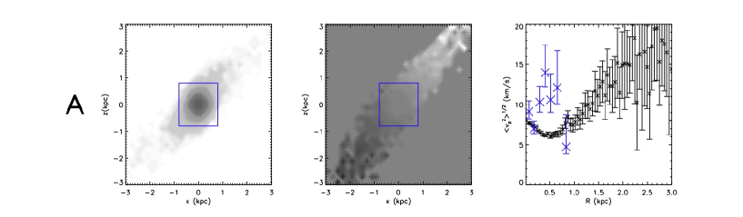
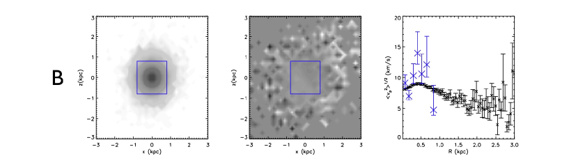
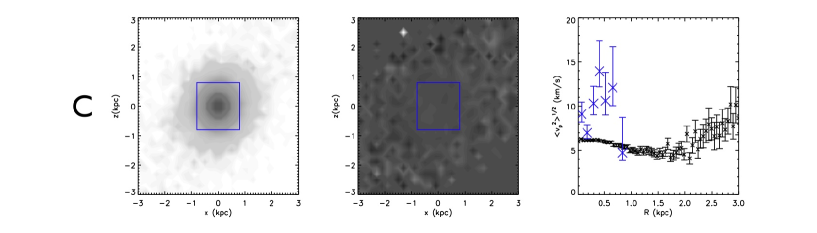
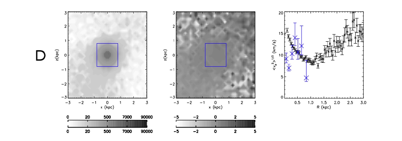
Figure 4: Projected surface density (left), velocity (middle) and velocity dispersion (right) for models A (top) through D (bottom). The grey contours show particle numbers per unit area (left) and velocities in km/s (middle). Over-plotted on the projected velocity dispersion plot (right) are the data for the Draco dSph galaxy taken from Wilkinson et al. (2004). The blue boxes overlaid on the contours mark approximate current observational limits. The projections shown are typical; different projections for model A are shown in Figure 6.

3.3 The choice of initial conditions: models A-D

We chose four models for our initial conditions labelled A-D as shown in Table 1 and Figure 3. In all models the density distribution for the stars and dark matter were given either by Plummer spheres (Binney & Tremaine, 1987) or by Split Power law profiles (SP) (Hernquist 1990, Saha 1992, Dehnen 1993 and Zhao 1996). The density-potential pairs for these distributions are given by respectively:

$$\rho_{\mathrm{plum}}=\frac{3M}{4\pi a^{3}}\frac{1}{(1+\frac{r^{2}}{a^{2}})^{5/2}}$$ (11)

$$\Phi_{\mathrm{plum}}=\frac{-GM}{\sqrt{r^{2}+a^{2}}}$$ (12)

$$\rho_{\mathrm{SP}}=\frac{M(3-\alpha)}{4\pi a^{3}}\frac{1}{(r/a)^{\alpha}(1+r/a)^{4-\alpha}}$$ (13)

$$\Phi_{\mathrm{SP}}=\frac{GM}{a(2-\alpha)}\left[(1+a/r)^{\alpha-2}-1\right]$$ (14)

where $M$ and $a$ are the mass and scale length in both cases, and $\alpha$ is the central log-slope for the SP profile (note that the SP profile always goes as $\rho_{\mathrm{SP}}\propto r^{-4}$ for $r\gg a$).

As detailed in section 1, each of these models was chosen to test a different scenario for the evolution of dSphs in the presence of tides. In all of the models, the dSph was placed on a plunging orbit which took it through the Milky Way disc. This ensured that both tidal stripping and shocking were important (see section 2). The initial conditions, orbit and output time for each of the models are given in Table 1. Models B and C placed the dSph on an orbit which is consistent with current constraints from the proper motion of Draco (Kleyna et al., 2001). However, these proper motion measurements are notoriously difficult and the errors large (see e.g. Piatek et al. 2002). Thus in models A and D, we also consider more extreme (i.e. more radial) orbits.

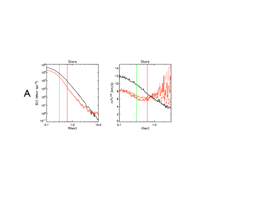
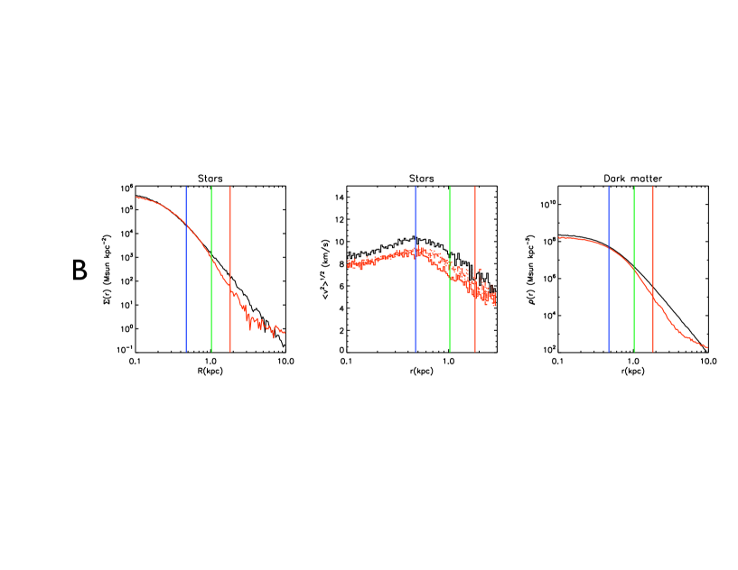
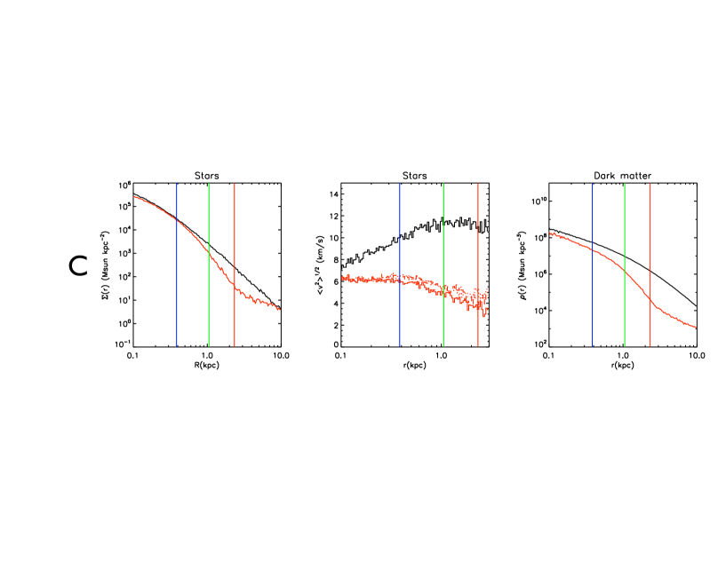
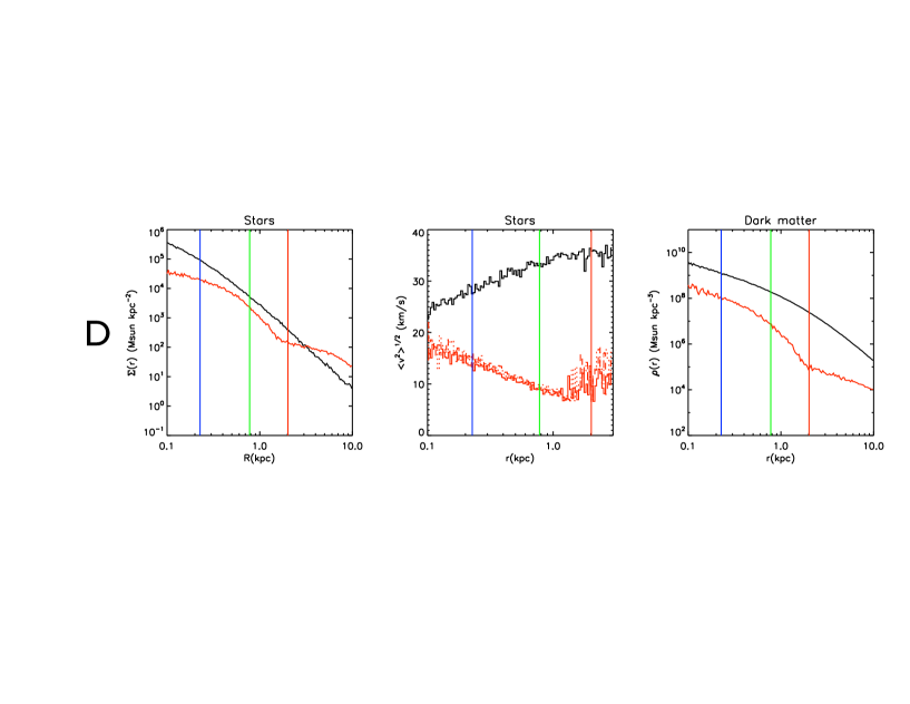
Figure 5: Projected surface brightness profile of the stars (left panel), velocity dispersion of the stars (middle panel) and the density profile of the dark matter (right panel). Over-plotted are three theoretical tidal radii calculated as described in Read et al. (2005); the blue/green/red vertical lines are for the prograde/radial/retrograde tidal radii respectively. The black lines show the initial conditions, while the red lines show the evolved profiles at the output times given in Table 1. In the velocity dispersion plot, the solid, dotted and dashed lines show the $r$, $\theta$ and $\phi$ components of the velocity dispersion respectively. Models A-D are shown from top to bottom. Model A did not contain any dark matter which is why no plot is shown for the dark matter in this case. The tidal radius for prograde star orbits (vertical blue line) cannot be seen for model A since it lies at very small radii (9 pc).

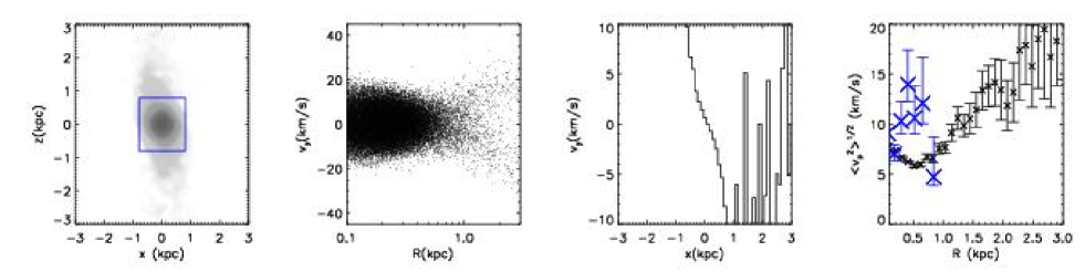
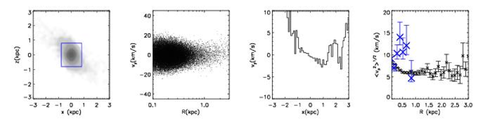
Figure 6: The effect of viewing projection for model A. Top panels show a typical projection; bottom panels show a rare projection which kinematically hides one of the tidal tails. From left to right panels show: projected surface density, individual projected star velocities, mean projected velocity and projected velocity dispersion. The grey contours show particle numbers per unit area as in Figure 4. Over-plotted on the projected velocity dispersion plot (right) are the data for the Draco dSph galaxy taken from Wilkinson et al. (2004). The blue boxes overlaid on the contours mark approximate current observational limits. Note that the velocity gradients shown here are averaged over the $y$ and $z$ coordinates and are necessarily different to the two dimensional gradients shown in Figure 4.

4 Results

The results for models A-D are presented in Figures 4 and 5. In Figure 4, we show the projected surface brightness (left panel), projected velocity (middle panel) and projected velocity dispersion (right panel) for the stars. For the projected velocity dispersion, the errors are determined from Poisson statistics. Models A-D are presented down the page. In Figure 5 we show the projected surface brightness profile for the stars (left panel), the true velocity dispersion of the stars (middle panel) and the density profile of the dark matter (right panel). For clarity on the plots, we compare the results of our simulations to data from the Draco dSph only, on the assumption that Draco is representative of the most dark matter dominated Local Group dSphs (see section 1 and Figure 1). In Figure 6 we show the effect of different viewing angles in projection on the sky, using model A as an example. In Figure 8 we show the mass loss, due to tides, as a function of time for all four models A-D.

4.1 The no-dark matter hypothesis: model A

In model A, we test the hypothesis that we can eliminate the need for dark matter in dSph galaxies by instead employing tidal heating to raise the velocity dispersions. One of the appealing aspects of such a model is that it produces tidally distorted isophotes, such as those which may have been seen in some dSphs (see e.g. Martínez-Delgado et al. 2001 and Palma et al. 2003).

In Figure 4, top left panel, we can see that distortions occur naturally in such a tidal model and the S-shaped isophotes caused by tides can be clearly seen in this projection. However, once the kinematic data are taken into account, it is clear that such a model runs into serious difficulties. The projected velocity shows a strong gradient (10 km/s/kpc) due to the near-dominant tidal arms, whereas no such velocity gradients have been observed in the Local Group dSphs so far (Wilkinson et al., 2004). Furthermore, the projected velocity dispersion rises out towards the edge of the light, whereas the Local Group dSphs like Draco have flat or falling projected velocity dispersions (see e.g. Wilkinson et al. 2004, Muñoz et al. 2005, Kleyna et al. 2004 and Figure 1). It is possible, however, that such tidal features could be hidden in projection. Figure 6 shows the effect of different viewing projections on the sky for model A. The top and bottom panels show two different projections: the top is a more typical projection, while the bottom, which kinematically hides one of the tidal tails, is more rare. By rare, we mean that such obscurations only occur for $\sim 1/5$ of all projection angles. While the orbit of any given dSph would rule out some projection angles, when studying the generic effect of tides on all of the Local Group dSphs, it seems reasonable to consider such random projections.

Notice from the middle left panels, that the primary cause of the rising velocity dispersion in projection is the cylindrical averaging which picks up both tidal tails. This is why, when a suitable projection is found which hides one of the tails, the velocity dispersion becomes flat rather than rising (bottom panels). In this case the velocity gradients are visible (middle right panel) only at large radii. Interior to $\sim 1$ kpc, the velocity gradient is less than $\sim 5$ km/s. Such a small velocity gradient would be difficult to detect observationally (Wilkinson et al., 2004). However, even this special projection is inconsistent with the data from Draco, UMi and Sextans which all show falling velocity dispersions in projection (see Figure 1).

It is worth recalling at this point that we are not trying to explicitly model the Draco, UMi or Sextans dSphs. Instead we show that the generic effect of tides is to produce velocity gradients and flat or rising projected velocity dispersions. That this is not seen in Draco, Sextans or UMi suggests that while tidal stripping may be important beyond the edge of the currently observed light ($\sim$1 kpc), it is unlikely to have been important within this radius.

An interesting feature of model A is that the small pericentre of the satellite (9 kpc) causes strong tidal shocks which over 10 Gyr lower the central density of the stars by a factor of $\sim 2$. This can be seen in Figure 5, top panels. These tidal shocks, as discussed in Read et al. (2005) wash out the tidal features which would otherwise be expected at the analytic tidal radii (blue, red and green vertical lines in Figure 5). However, the effects of tides can still be seen in the velocity dispersions. Notice that tangential anisotropy, which should be present beyond the prograde stripping radius is present at all radii over the satellite (see section 2.1). For model A, the prograde stripping radius lies at just 9 pc and hence does not show up in Figure 5.

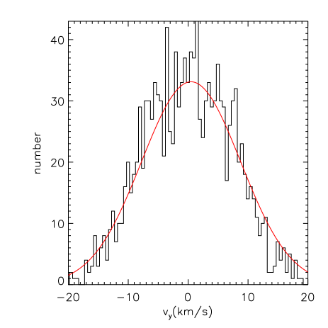
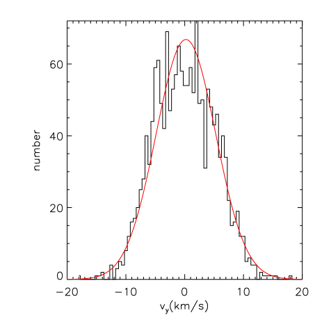
Figure 7: Histogram of the stellar velocities in a 0.2 kpc bin at 1 kpc for model B (left) and model C (right). Over-plotted are Gaussian fits in both cases (red lines).

4.2 Weak tides: models B and C

In models B and C we consider the effect of weak tides on the Local Group dSph galaxies. In this case we imagine that tides gently shape the outer regions of dSphs over a Hubble time.

In Figure 4, second and third panels from top, we can see that tides have little affected models B and C. The surface brightness distributions are nearly spherical, as in the initial conditions, and there are no visible velocity gradients across the galaxy. Tidal heating of the outermost stars is present in both models from about $\sim 2$ kpc outwards. Notice that in neither model is there a drop in the projected velocity dispersion. The decline in model A was present in the initial conditions and is not as sharp as that seen in the data from Draco.

This can also be seen in Figure 5, second and third panels from top. Notice that, as in model A, tangential velocity anisotropy appears at the prograde stripping radius (vertical blue line) in both models B and C. Notice also the action of tidal shocks, particularly on the dark matter in model C. As the satellite is puffed up by shocks, its velocity dispersion at all radii is lowered. This may seem counter-intuitive at first: the satellite is heated by tidal shocks and yet its velocity dispersion falls. However, it is the subsequent expansion of the satellite after the injection of energy from the tidal shock which causes a drop in its velocity dispersion at a given radius.

Notice further that it is only in projection that the velocity dispersions appear hot beyond the tidal radius. The true velocity dispersions are still gently falling, as in the initial conditions, at this point. This occurs for two reasons. First, and this is usually the dominant effect for a given projection, the cylindrically averaged tidal tails cause the projected velocity dispersion to rise (see Figure 6). Second, the onset of tangential anisotropy makes the outermost stars appear hot in projection. This second effect is only important when the tidal tails are viewed along the line of sight, thereby minimising the extent to which they can be observed in projection.

This is interesting: in all models tidal stripping leads to a rising or flat projected velocity dispersion. There is never a sharp decline such as that observed in the Draco, UMi and Sextans dSphs (see section 1). We now discuss why tidal stripping always leads to hot stars in projection by considering three mechanisms by which tidal stripping might have led instead to the opposite - namely a cold outer point in the projected velocity dispersion.

(i) The outer-most point is the result of a chance projection effect between the galaxy and its tidal tail along the line of sight.

We explicitly checked for this by searching over 5 degree projections every half orbital period for both models B and C and found no sharp features at any output time. If a projection effect could cause such a sharp drop it would be very rare and, while one could envisage this for one Local Group dSph galaxy, the fact that such a sharp feature has been observed in at least three renders this possibility unlikely.

(ii) The dSph galaxy is on a significantly plunging orbit. The outermost stars are heated up by a disc shock as the dSph plunges through the Milky Way disc. The dSph galaxy then moves out towards apocentre and the hot outer stars escape leaving a cold population behind.

This hypothesis was presented in Wilkinson et al. (2004) and formed one of the motivations for this current work. The output time chosen for models B and C has been specifically selected to test this hypothesis. We choose a time when the dwarf galaxy has spent a large amount of time away from the Milky Way disc and the outermost stars heated by the last passage have had time to escape. The hypothesis is falsified for three reasons. First, for the case of models B and C, tidal shocking replenishes stars beyond the tidal radius and so there is always a source of hot tidal stars which mask any cold populations. Secondly, the image of a sharp edge to the satellite beyond which a cold population of stars might exist is not correct. As shown in a companion paper (Read et al. 2005; and see also section 2), the tidal radius of the satellite depends on the orbit of the stars within the satellite. This leads to a continuum of tidal radii and, therefore, no sharp edge to the satellite. Finally, even if there were such a sharp edge, and tidal shocking did not refill stars beyond the tidal radius, there would be on average more stars on circular orbits than radial orbits at the tidal radius and the distribution would still appear hot in projection. We explicitly checked that this is indeed the case by considering some more extreme orbits with very large apocentres ($260$ kpc), and pericentres large enough to make the effect of tidal shocking negligible ($35$ kpc). Even in these cases the projected velocity dispersions are flat or rising, for the reasons presented above. As a final check, we considered also only the bound stars. Plotting only these removes the hot tidal tail, but still does not lead to cold outer stars in projection.

We conclude that if such cold outer populations in dSph galaxies are real then they cannot have formed as a result of tidal effects which always produce stars which appear hot in projection.

(iii) The velocity distribution of the outer-most stars is highly non-Gaussian, with a significant tail of high velocity stars. This could lead to a large fraction of stars being deemed non-members of the dSph galaxy and excluded from the data analysis, leading to a spurious detection of a cold outer point.

To test this hypothesis, we plot the distribution of line of sight velocities in a 0.2 kpc-wide bin at a projected radius of 1 kpc for models B and C (Figure 7). Over-plotted are Gaussian fits to the binned data in both cases (red lines). The distributions are close to Gaussian: neither shows a strong asymmetric tail. Similar results were found at other radii. We conclude that it is unlikely that a significant fraction of high velocity stars would be excluded as members of Draco from an observational data analysis.

4.3 Strong tidal shocking: model D

In model D, we consider the hypothesis that the progenitors of dSph galaxies were much more massive than they appear at the present time. As can be seen in models A, B and C, the action of tidal shocks puffs up the satellite and lowers the velocity dispersion at all radii. In model D, we start with a satellite which has a very large central velocity dispersion which is not consistent with current data from the Local Group dSphs. We consider the case where this velocity dispersion is lowered over time by the action of tidal shocks such that it becomes consistent with current data now.

As we showed in section 2.2, it is possible to find a regime where tidal shocks dominate over stripping interior to the stars. The existence of such a regime is demonstrated numerically by model D.

In Figure 4, bottom panels, we can see that the satellite has been little affected by tidal stripping inside $\sim 1$ kpc. It retains smooth spherical contours and shows no strong velocity gradients. Beyond $\sim 1$ kpc, tidal stripping becomes significant and the outer stars appear hot in projection. However, in Figure 5, we can see that tidal shocking has been much more important than the stripping over a Hubble time. The central density of the dark matter has lowered by a factor of $\sim 10$, and similarly for the stars. The velocity dispersion of the stars is lower at all radii, but notice that the central value is still high - similar to the initial conditions. This reflects the presence initially of a central dark matter cusp. This allows the density at the centre of the satellite to become high enough that tidal shocking is less effective, even over very long timescales and for this extreme orbit (recall that the satellite pericentre for model D is just 6 kpc). Finally, notice that despite such strong tidal shocks, the central dark matter cusp persists, albeit at a lower normalisation. This agrees with findings from previous authors (Kazantzidis et al., 2004). It is this central dark matter cusp which leaves the satellite with a central velocity dispersion which is too large to be consistent with data from any of the Local Group dSphs observed so far. In a similar model which we ran with a central dark matter core instead of a cusp, much better agreement was obtained. We will return to this issue in section 5.

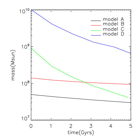
Figure 8: Total bound mass (stars and dark matter) as a function of time for models A-D.

In model D, as in models A and C, the satellite loses significant mass over a Hubble time as a result of tidal stripping and shocking. This is shown in Figure 8, where we compare the bound mass as a function of time for each of the models A-D. At the output time shown, the bound mass of the satellite in model D has been reduced by a factor of $\sim 10$. This explains why the final velocity dispersion matches the data from Draco, while the initial dispersions were much too high. Such mass loss continues steadily over the whole simulation time due to the action of shocks.

5 Discussion

5.1 Sagittarius: a tidally stripped dSph galaxy

We know of one Local Group dSph which is definitely undergoing tidal stripping: the Sagittarius dwarf (Ibata et al. 2001 and Law et al. 2005). Its tidal streams are quite cold, giving a flat velocity dispersion of $\sim 10$ km/s (Law et al., 2005), consistent with its central value (Ibata et al., 1997). Furthermore the velocity gradients across its minor axis ($\pm 1$ kpc) seem to be only $\sim 3$ km/s (Ibata et al., 1997).

Olszewski (1998) and Ibata et al. (1997) have argued that these data for the Sagittarius dwarf must imply large amounts of dark matter, similar to the other dSphs, such that the effects of tides become hard to detect within the body of the Sagittarius dSph. An alternative view is that even strong tides do not produce measurable effects in the kinematics, even out to radii which begin to sample the tidal tails. As we have shown in this paper, this second view is possible if Sagittarius is favourably aligned (see Figure 6). One might speculate that the other dSphs could be undergoing tidal disruption but the signs of it are masked in projection. Such favourable alignments seem unlikely to be the case for all of the Local Group dSphs. Furthermore, in at least three dSphs (UMi, Draco and Sextans), the velocity dispersion is actually falling. This is inconsistent with strong tidal effects interior to $\sim$ 1kpc.

5.2 The tidal model

Kroupa (1997) found that tidal models for the formation of dSphs without dark matter can reproduce the spatial and kinematic observations. Central to such models is the idea that the dSph galaxy starts out as a high density star cluster. Through tidal shocking and stripping the star cluster is heated up and becomes almost completely unbound. In such a scenario, high projected velocity dispersions are to be expected (c.f. model A). However, these do not correspond to a large mass for the satellite since the tidally heated stars are not bound and the Jeans equations or distribution function modelling do not apply.

In our simulations, we find similar results to those presented in Kroupa (1997). Kroupa (1997) also finds rising (cylindrically averaged) projected velocity dispersions for tidally stripped and shocked dSphs (see their Figure 10). It is the new data from the Local Group dSphs, which were not available to Kroupa (1997), that rule out these dark matter free tidal models, not an improvement in the simulations. Even using favourable projections (as in Figure 6), it is not possible to have a falling projected velocity dispersion in the tidal model - a result which concords with other studies of the tidal model too (see e.g. Fleck & Kuhn 2003).

Piatek & Pryor (1995) also argued against a dark matter free tidal origin for the dSphs. They found significant velocity gradients in their simulations which were inconsistent with observations. As in Kroupa (1997), we find that it is possible to hide such velocity gradients using suitable projections. Thus it is the existence of cold outer populations in projection which provide the hardest challenge for such tidal models, rather than the velocity gradients alone.

Finally, for Draco, Klessen et al. (2003) showed that the tidal model will not work since Draco cannot be very extended along the line of sight (something which is required in any projection which disguises the velocity gradients and significant tidal tails, but in which the velocity dispersion is inflated due the inclusion (in projection) of stars from the tidal tails). Through detailed modelling of Draco, Mashchenko et al. (2005) also find that the tidal model is not favourable. Here, we confirm these results, and extend the list of tidal stripping-free dwarfs to include UMi and Sextans.

5.3 Mass bounds from tides

It is interesting to now turn the problem of the cold outer stars in Draco, Sextans and UMi on its head. The presence of such stars tells us that either the tidal radius must lie beyond this point, or that the cold point was formed recently and has not had time to be disrupted by tides. The latter seems unlikely: Draco and UMi have very old stellar populations ($\lower 2.15277pt\hbox{$\;\buildrel>\over{\sim}\;$}10$ Gyrs), which suggests that any baryonic process which might cause such a cold point must have occurred long ago. As such, in this section, we discuss the implications of these Local Group dSphs having tidal radii $\lower 2.15277pt\hbox{$\;\buildrel>\over{\sim}\;$}0.8$ kpc, which is the current observational edge for kinematic observations in these galaxies. For brevity from here on, we use the term ‘Local Group dSphs’ to mean Draco, UMi and Sextans.

From Figures 4 and 5, we can see that the tidal heating of stars starts at the prograde stripping radius (this is where the tangential velocity anisotropy begins - see section 2.1 and Read et al. 2005). Thus from here on, by ‘tidal radius’ we refer to the prograde stripping radius.

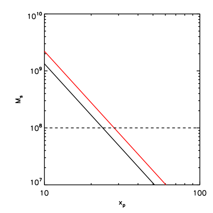
Figure 9: A lower mass bound on the Local Group dSphs as a function of their orbital pericentres. The red line is for highly eccentric dSph orbits ($e=1$) while the black is for circular orbits ($e=0$). The mass limits were obtained from the prograde tidal radius (see equation 1 with $\alpha=1$). Also marked is the approximate lower bound on the mass obtained from stellar kinematics and distribution function models for Draco (black dashed line; and see Kleyna et al. 2001). UMi and Sextans have similar lower bounds.

The tidal radius is a function of the satellite and Milky Way potentials, and the orbit of the satellite. However, assuming point masses leads to, at most, errors of the order of 2-3 in the prograde tidal radius (Read et al., 2005). Thus, rearranging equation 1 should give us a reasonable lower bound on the mass of Local Group dSphs within the tidal radius, as a function of their orbital pericentre. This is plotted in Figure 9. It is a lower bound because the tidal radius must be greater than the outermost measured kinematic point (in order to preserve a cold outer point) in the Local Group dSphs, which we take to be $\sim 0.8$ kpc.

Since we have shown that tidal stripping is not likely to act interior to $\sim 0.8$ kpc in at least Draco, UMi and Sextans, this suggests that these galaxies are close to equilibrium and a mass bound from the Jeans equations or distribution function modelling is sound. What, then, can we learn from a mass bound from tides which is degenerate with the orbit of the dSph and the potential of the Milky Way, both of which are poorly constrained? From Figure 9, we can see that, if the orbital pericentre of the Local Group dSphs is $\lower 2.15277pt\hbox{$\;\buildrel>\over{\sim}\;$}30$ kpc, then we learn nothing new from the tidal mass bound: tidal stripping and shocking are both negligible for all satellite masses $\lower 2.15277pt\hbox{$\;\buildrel>\over{\sim}\;$}10^{8}$M_⊙ - the mass bound obtained from distribution function modelling. However, if the pericentre of the orbit is $\lower 2.15277pt\hbox{$\;\buildrel<\over{\sim}\;$}30$kpc, then the satellite must have been more massive in the past than it is at present in order to have survived intact on its current orbit. Thus for small pericentre orbits, the tidal mass bound is a bound on the dSph’s initial mass, before tidal stripping and shocking. That it is now less massive than this then means that tidal shocking must have acted to lower the central mass and velocity dispersion over a Hubble time (as in models C and D).

5.4 Can dSphs reside in the most massive substructure halos?

The dark matter halo in model D had a total mass of $10^{10}$M_⊙, consistent with the most massive dark matter halos predicted by cosmological simulations to surround the Milky Way (Klypin et al., 1999). The initial mass within $0.8$ kpc for model D was $10^{9}$M_⊙, while after significant tidal shocking on its extreme orbit (with pericentre of 6.5 kpc), the final mass within $0.8$ kpc was $\sim 10^{8}$M_⊙. This final mass is consistent with current mass estimates for Draco, UMi and Sextans, but its concentration is not. The survival of the central dark matter density cusp in model D ensured that the central velocity dispersion of the surviving dSph galaxy was too large, even after extreme tidal shocking.

Interestingly, there may be tentative evidence that the UMi dSph has a centrally cored dark matter density profile, rather than a cusp (Kleyna et al., 2003). If this is the case then it is possible that UMi started out with total mass $10^{10}$M_⊙ and had its velocity dispersion lowered through the action of tidal shocks. With a central dark matter density core, rather than a cusp, such shocks can lower even the central velocity dispersion to 10 km/s in accord with the measured values for the Local Group dSphs. Thus it is only possible for the dSphs to inhabit the most massive substructure halos if they have density profiles which are not consistent with simple cosmological predictions.

A natural consequence of such strong tidal shocking is that we can expect a correlation between the central surface brightness of the Local Group dSphs and their pericentre: dSphs which pass closer to their host galaxies will show lower central surface brightnesses. While the orbits of the Local Group dSphs remain poorly constrained and so their pericentres are not well known, a correlation between central surface brightness and distance to the nearest host galaxy has been observed (Bellazzini et al. 1996 and Mcconnachie & Irwin 2005). While there are many possible explanations for such a correlation (for example selection effects), a plausible explanation would be tidal shocking.

Finally, tidal shocks could provide the necessary physics to remove angular momentum from the dSphs and transform them from an initially disc-like population to a spheroidal population as in Mayer et al. (2001a) and Mayer et al. (2001b). We argue in this paper that the Local Group dSphs have not been significantly stripped interior to 1 kpc, but this need not invalidate the tidal transformation model proposed by Mayer et al. (2001a).

6 Conclusions

We have compared the results from a suite of N-body simulations of the tidal stripping and shocking of two-component, spherical, dwarf galaxies in orbit around a Milky Way like galaxy, with recently obtained kinematic data for the Local Group dwarf spheroidals (dSphs).

Our main findings are summarised below:

(i) Tidal stripping always leads to flat or rising projected velocity dispersions beyond a critical radius; it is $\sim 5$ times more likely, over random projections, that the cylindrically averaged projected dispersion will rise than be flat.

(ii) In several of the dSphs observed so far, there appears to be a sharp fall-off in the projected velocity dispersion at large radii. If such a feature is real and not a statistical artifact, it would be rapidly destroyed by tidal stripping - tidal stripping cannot have acted interior to the currently visible light in these galaxies (interior to $\sim 1$ kpc).

(iii) By contrast, there exists a regime in which tidal shocking can be important interior to the visible light, even when tidal stripping is not. This could explain the observed correlation for the Local Group dSphs between central surface brightness and distance from the nearest large galaxy (Bellazzini et al. 1996 and Mcconnachie & Irwin 2005).

(iv) It is possible for dSphs to reside within the most massive substructure dark matter halos ($\sim 10^{10}$M_⊙) and have their velocity dispersions lowered through the action of tidal shocks, but only if they have a central density core in their dark matter, rather than a cusp. A central density cusp persists even after unrealistically extreme tidal shocking and leads to central velocity dispersions which are too high to be consistent with data from the Local Group dSphs. dSphs can reside within cuspy dark matter halos if their halos are less massive ($\sim 10^{9}$M_⊙) and therefore have smaller central velocity dispersions initially.

(v) A tidal origin for the formation of the Local Group dSphs in which they contain no dark matter is strongly disfavoured. This is because such a formation scenario requires very strong tidal stripping, the effects of which are at odds with the latest data from the Local Group dSphs.

7 Acknowledgements

JIR and MIW would like to thank PPARC for grants which have supported this research. We would like to thank the annonymous referee for useful comments which led to this final version.

References

- Aarseth (1999) Aarseth S. J., 1999, PASP, 111, 1333
- Aguilar & White (1986) Aguilar L. A., White S. D. M., 1986, ApJ, 307, 97
- Bellazzini et al. (1996) Bellazzini M., Fusi Pecci F., Ferraro F. R., 1996, MNRAS, 278, 947
- Binney & Tremaine (1987) Binney J., Tremaine S., 1987, Galactic dynamics. Princeton, NJ, Princeton University Press, 1987, 747 p.
- Dehnen (1993) Dehnen W., 1993, MNRAS, 265, 250
- Dehnen (2000) Dehnen W., 2000, ApJ, 536, L39
- Fleck & Kuhn (2003) Fleck J.-J., Kuhn J. R., 2003, ApJ, 592, 147
- Gnedin et al. (1999) Gnedin O. Y., Hernquist L., Ostriker J. P., 1999, ApJ, 514, 109
- Gnedin et al. (1999) Gnedin O. Y., Lee H. M., Ostriker J. P., 1999, ApJ, 522, 935
- Gnedin & Ostriker (1997) Gnedin O. Y., Ostriker J. P., 1997, ApJ, 474, 223
- Grebel et al. (2003) Grebel E. K., Gallagher J. S., Harbeck D., 2003, AJ, 125, 1926
- Hayashi et al. (2003) Hayashi E., Navarro J. F., Taylor J. E., Stadel J., Quinn T., 2003, ApJ, 584, 541
- Hernquist (1990) Hernquist L., 1990, ApJ, 356, 359
- Hernquist (1993) Hernquist L., 1993, ApJS, 86, 389
- Ibata et al. (2001) Ibata R., Lewis G. F., Irwin M., Totten E., Quinn T., 2001, ApJ, 551, 294
- Ibata et al. (1997) Ibata R. A., Wyse R. F. G., Gilmore G., Irwin M. J., Suntzeff N. B., 1997, AJ, 113, 634
- Irwin & Hatzidimitriou (1995) Irwin M., Hatzidimitriou D., 1995, MNRAS, 277, 1354
- Kazantzidis et al. (2004) Kazantzidis S., Magorrian J., Moore B., 2004, ApJ, 601, 37
- Kazantzidis et al. (2004) Kazantzidis S., Mayer L., Mastropietro C., Diemand J., Stadel J., Moore B., 2004, ApJ, 608, 663
- King (1962) King I., 1962, AJ, 67, 471
- Klessen et al. (2003) Klessen R. S., Grebel E. K., Harbeck D., 2003, ApJ, 589, 798
- Kleyna et al. (2001) Kleyna J. T., Wilkinson M. I., Evans N. W., Gilmore G., 2001, ApJ, 563, L115
- Kleyna et al. (2004) Kleyna J. T., Wilkinson M. I., Evans N. W., Gilmore G., 2004, MNRAS, 354, L66
- Kleyna et al. (2003) Kleyna J. T., Wilkinson M. I., Gilmore G., Evans N. W., 2003, ApJ, 588, L21
- Klypin et al. (1999) Klypin A., Kravtsov A. V., Valenzuela O., Prada F., 1999, ApJ, 522, 82
- Kravtsov et al. (2004) Kravtsov A. V., Gnedin O. Y., Klypin A. A., 2004, ApJ, 609, 482
- Kroupa (1997) Kroupa P., 1997, New Astronomy, 2, 139
- Kuhn & Miller (1989) Kuhn J. R., Miller R. H., 1989, ApJ, 341, L41
- Kuijken & Dubinski (1995) Kuijken K., Dubinski J., 1995, MNRAS, 277, 1341
- Law et al. (2005) Law D. R., Johnston K. V., Majewski S. R., 2005, ApJ, 619, 807
- Mcconnachie & Irwin (2005) Mcconnachie A., Irwin M., 2005, . In preparation.
- Martínez-Delgado et al. (2001) Martínez-Delgado D., Alonso-García J., Aparicio A., Gómez-Flechoso M. A., 2001, ApJ, 549, L63
- Mashchenko et al. (2005) Mashchenko S., Sills A., Couchman H. M. P., 2005
- Mateo (1998) Mateo M. L., 1998, ARA&A, 36, 435
- Mayer et al. (2001a) Mayer L., Governato F., Colpi M., Moore B., Quinn T., Wadsley J., Stadel J., Lake G., 2001a, ApJ, 559, 754
- Mayer et al. (2001b) Mayer L., Governato F., Colpi M., Moore B., Quinn T., Wadsley J., Stadel J., Lake G., 2001b, ApJ, 547, L123
- Moore et al. (1999) Moore B., Ghigna S., Governato F., Lake G., Quinn T., Stadel J., Tozzi P., 1999, ApJ, 524, L19
- Muñoz et al. (2005) Muñoz R. R., Frinchaboy P. M., Majewski S. R., Kuhn J. R., Chou M.-Y., Palma C., Sohn S. T., Patterson R. J., Siegel M. H., 2005, ApJ, 631, L137
- Nagai & Miyamoto (1976) Nagai R., Miyamoto M., 1976, PASJ, 28, 1
- Oh et al. (1995) Oh K. S., Lin D. N. C., Aarseth S. J., 1995, ApJ, 442, 142
- Olszewski (1998) Olszewski E. W., 1998, in ASP Conf. Ser. 136: Galactic Halos Internal Kinematics of Dwarf Spheroidal Galaxies. pp 70–+
- Ostriker et al. (1972) Ostriker J. P., Spitzer L. J., Chevalier R. A., 1972, ApJ, 176, L51+
- Palma et al. (2003) Palma C., Majewski S. R., Siegel M. H., Patterson R. J., Ostheimer J. C., Link R., 2003, AJ, 125, 1352
- Piatek & Pryor (1995) Piatek S., Pryor C., 1995, AJ, 109, 1071
- Piatek et al. (2002) Piatek S., Pryor C., Olszewski E. W., Harris H. C., Mateo M., Minniti D., Monet D. G., Morrison H., Tinney C. G., 2002, AJ, 124, 3198
- Pontzen et al. (2005) Pontzen A., Read J. I., Ricotti M., Viel M., 2005, . In preparation.
- Power et al. (2003) Power C., Navarro J. F., Jenkins A., Frenk C. S., White S. D. M., Springel V., Stadel J., Quinn T., 2003, MNRAS, 338, 14
- Press et al. (1992) Press W. H., Teukolsky S. A., Vetterling W. T., Flannery B. P., 1992, Numerical recipes in C. The art of scientific computing. Cambridge: University Press, —c1992, 2nd ed.
- Read et al. (2005) Read J. I., Wilkinson M. I., Evans N. W., Gilmore G., Kleyna J. T., 2005, . In preparation.
- Saha (1992) Saha P., 1992, MNRAS, 254, 132
- Spitzer (1987) Spitzer L., 1987, Dynamical evolution of globular clusters. Princeton, NJ, Princeton University Press, 1987, 191 p.
- Springel et al. (2001) Springel V., Yoshida N., White S. D. M., 2001, New Astronomy, 6, 79
- Stoehr et al. (2002) Stoehr F., White S. D. M., Tormen G., Springel V., 2002, MNRAS, 335, L84
- Wilkinson et al. (2004) Wilkinson M. I., Kleyna J. T., Evans N. W., Gilmore G. F., Irwin M. J., Grebel E. K., 2004, ApJ, 611, L21
- Zhao (1996) Zhao H., 1996, MNRAS, 278, 488