Weak lensing mass reconstructions of the ESO Distant Cluster Survey

We present weak lensing mass reconstructions for the 20 high-redshift clusters in the ESO Distant Cluster Survey. The weak lensing analysis was performed on deep, 3-color optical images taken with VLT/FORS2, using a composite galaxy catalog with separate shape estimators measured in each passband. We find that the EDisCS sample is composed primarily of clusters that are less massive than those in current X-ray selected samples at similar redshifts, but that all of the fields are likely to contain massive clusters rather than superpositions of low mass groups. We find that 7 of the 20 fields have additional massive structures which are not associated with the clusters and which can affect the weak lensing mass determination. We compare the mass measurements of the remaining 13 clusters with luminosity measurements from cluster galaxies selected using photometric redshifts and find evidence of a dependence of the cluster mass-to-light ratio with redshift. Finally we determine the noise level in the shear measurements for the fields as a function of exposure time and seeing and demonstrate that future ground-based surveys which plan to perform deep optical imaging for use in weak lensing measurements must achieve point-spread functions smaller than a median of $0\aas@@fstack{\prime\prime}6$ FWHM.

1 Introduction

The discovery of massive ($>10^{15}\mathrm{M}_{\odot}$), high-redshift ($z>0.6$) clusters in serendipitous X-ray surveys (eg the Einstein Medium Sensitivity Survey (EMSS), Gioia et al. 1990) resulted in constraints on the evolution of structure in the Universe that excluded an Einstein-de Sitter model and favored a low mass-density model (Oukbir & Blanchard 1992; Eke et al. 1996). Further constraints on cosmological models have come from measuring the evolution, or lack there of, of various traits of the clusters, such as the X-ray gas temperature and gas mass fraction (Evrard et al. 2002; Henry 2000).

These studies, however, have faced two potentially serious problems. The first is that the current X-ray surveys are only able to detect the most massive clusters at high-redshift, which often results in a mismatch in the mass range between these high-redshift clusters and the lower redshift samples to which they are compared. The ESO Distant Cluster Survey (EDisCS) is a sample of 20 fields likely to contain high-redshift clusters, chosen from the optically selected Las Campanas Distant Cluster Survey (Gonzalez et al. 2001), which detected clusters from smoothed overdensities in the sky level of shallow optical exposures. The LCDCS covered roughly the same sky area as the deepest pointings in the EMSS but found an order of magnitude more high-redshift clusters. As a result, the clusters in EDisCS should, on average, be of lower mass than the X-ray selected samples, and thus more directly comparable to lower redshift samples.

The second problem is that the high-redshift clusters are being observed at a time when structure formation is much more dynamic than it is today, so it is uncertain how well properties such as the X-ray gas temperature and cluster galaxy velocity dispersion, which depend upon the cluster being in virial equilibrium, relate to the mass of the cluster. Thus, to check for evolution in such cluster properties, one needs a measurement of the mass of the clusters using a method that does not require the cluster to be in a particular dynamical state. Weak gravitational lensing, in which one measures the distortion in the shapes of background galaxies by the gravitational potential of the cluster, provides a means to do this.

In this paper we use the deep optical VLT/FORS2 imaging from EDisCS to measure the gravitational shear field produced by the clusters and so derive mass estimates for them. In Section 2 we discuss the optical image reduction and object detection. In Section 3 we discuss the weak lensing analysis and present measurements of the mass and optical luminosity of the clusters. Results for the intermediate redshift ($z\sim 0.5$) clusters are discussed in Section 4, and those for the higher redshift sample in Section 5. Discussion of the results and potential systematic errors in the sample are given in Section 6. Throughout this paper we assume a $\Omega_{\mathrm{m}}=0.3,\Lambda\ =0.7,H_{0}=70\mathrm{km/s/Mpc}$ cosmology and give all errors as $1\sigma$ unless otherwise stated.

2 Data Reduction

2.1 Image Reduction and Object Detection

We use deep VLT/FORS2 images of the EDisCS clusters. Details of image acquisition and reduction process are described in White et al. (2004). A summary of the exposure times and PSF sizes for each of the three passbands for all twenty cluster fields is given in Table 1. For the weak lensing analysis, we make one alteration to the image reduction process compared to that used for the photometric analysis, which is to perform a smoothed sky subtraction on the individual input images before co-addition. This is done by using the IMCAT (http://www.ifa.hawaii.edu/$\sim$kaiser/imcat) findpeaks peak–finder inverted to find local minima on the images after being smoothed with a $1\arcsec$ Gaussian. Two images of the minima are then created, one with the minima values in the pixel locations where they are found and one in which the pixels with minima are set to 1, and both are smoothed with a $6\aas@@fstack{\prime\prime}8$ Gaussian. The smoothed minima image is then divided by the smoothed weight image to produce an image of the sky, which is subtracted from the original image. This process removes all small scale fluctuations in the sky from the input images along with extended stellar (and larger galaxy) halos and any intra-cluster light. This step was necessary to minimize the error in determining the second moments of the surface brightness of the galaxies, for which we assume the sky background can be modeled with a linear slope across the galaxy. An ultra-deep image was also created by co-adding the input images from all three passbands, weighted by the inverse of the square of the sky-noise in each image.

Table 1: Exposure times and PSF FWHM

$z\sim 0.5$ clusters
cluster	$I$		$V$		$B$
name	$t_{\mathrm{exp}}$ (m)	FWHM (″)	$t_{\mathrm{exp}}$ (m)	FWHM (″)	$t_{\mathrm{exp}}$ (m)	FWHM (″)
CLJ1018.8-1211	60	0.77	60	0.80	45	0.80
CLJ1059.2-1253	60	0.75	60	0.85	45	0.80
CLJ1119.3-1129	45	0.58	45	0.52	40	0.58
CLJ1202.7-1224	45	0.64	45	0.75	45	0.70
CLJ1232.5-1250	45	0.52	50	0.63	45	0.56
CLJ1238.5-1144	45	0.54	45	0.63	45	0.61
CLJ1301.7-1139	45	0.56	45	0.64	45	0.58
CLJ1353.0-1137	45	0.58	45	0.68	45	0.60
CLJ1411.1-1148	45	0.48	45	0.60	45	0.59
CLJ1420.3-1236	45	0.74	45	0.80	45	0.62
$z>0.6$ clusters
cluster	$I$		$R$		$V$
name	$t_{\mathrm{exp}}$ (m)	FWHM (″)	$t_{\mathrm{exp}}$ (m)	FWHM (″)	$t_{\mathrm{exp}}$ (m)	FWHM (″)
CLJ1037.9-1243	120	0.56	130	0.54	120	0.55
CLJ1040.7-1155	115	0.62	120	0.72	120	0.62
CLJ1054.4-1146	115	0.72	150	0.78	120	0.67
CLJ1054.7-1245	115	0.50	110	0.77	120	0.79
CLJ1103.7-1245	115	0.64	120	0.75	130	0.83
CLJ1122.9-1136	115	0.65	115	0.70	120	0.71
CLJ1138.2-1133	125	0.60	110	0.68	120	0.58
CLJ1216.8-1201	115	0.60	110	0.72	130	0.68
CLJ1227.9-1138	145	0.74	130	0.83	155	0.73
CLJ1354.2-1230	115	0.66	120	0.70	125	0.70

We detected objects in the ultra-deep images using SExtractor (Bertin & Arnouts 1996) set to find groups of three contiguous pixels that are $1\sigma$ above the sky-level. SExtractor was then used in two-image mode, with the ultra-deep image as the detection image, to measure the magnitudes, in both a $1\arcsec$ radius aperture and to an isophotal limit of $1\sigma$ in the ultra-deep image, for the objects in all three passbands. These produced catalogs with $\sim 110$ objects/sq. arcmin for the intermediate redshift clusters and $\sim 200$ objects/sq. arcmin for the high redshift clusters, with the majority of the objects being noise peaks. We determined the significance and size of each object in each passband by convolving the images with a series of Mexican-hat filters and determining the smoothing radius, $r_{\mathrm{g}}$, at which the filtered objects achieved maximum significance, $\nu$. The catalogs were then cut by removing all of the objects that are measured as having a smaller smoothing radius than the stars in all of the passbands, those which did not reach a significance of $10\sigma$ in at least one passband, and those which had a bad or saturated pixel or image border within an aperture of radius $3r_{\mathrm{g}}$. For each surviving object, typically $\sim 40\%$ of the detected objects, we measured a local sky level, flux within an aperture of radius $3r_{\mathrm{g}}$, and a $50\%$ encircled light radius, $r_{\mathrm{h}}$, in each passband. Stars were separated from galaxies by selection in $r_{\mathrm{h}}$, with only objects selected as stars in all three passbands being designated stars, and objects selected as stars in only one or two passbands having their significances set to 0 for those passbands.

The next step was to measure the reduced shear $\@vec{g}$, corrected for PSF smearing, for each object in each passband separately. The objects had their zeroth, second, and fourth moments, weighted by a Gaussian with $\sigma=r_{\mathrm{g}}$, measured and used to construct ellipticities, $\@vec{e}$, and shear and smear tensors as per the KSB technique (Kaiser et al. 1995). Stellar ellipticities, shear, and smear tensors were measured over the full range of weight function sizes used in the galaxy measurements, and in all subsequent steps the stellar ellipticities and tensors used in the KSB corrections are those which have the same weight function size as the galaxy being corrected. We determined the PSF ellipticity field by fitting the stellar ellipticities with a bi-cubic polynomial, which was then scaled by the ratio of galaxy to stellar smear tensors and subtracted from the galaxy ellipticities (Kaiser et al. 1995). A shear susceptibility tensor, $\@tens{P}^{\gamma}$ (Luppino & Kaiser 1997), was created for each galaxy. Because $\@tens{P}^{\gamma}$ is extremely noisy, instead of calculating $\@vec{g}_{i}={\@tens{P}^{\gamma}_{ij}}^{-1}\@vec{e}_{j}$ for each object from its measured $\@tens{P}^{\gamma}$ one needs to average the $\@tens{P}^{\gamma}$s of galaxies with similar light profiles. Since one expects that the shear susceptibility tensor depends mainly on the size and shape of the object, we fit each component of $\@tens{P}^{\gamma}_{ij}$ as a bi-pentic polynomial of $r_{\mathrm{g}}$ and $e_{j}$ and use the values of the fitted components. The final reduced shear measurement for each galaxy was then created from a weighted mean of the reduced shear in each passband, weighting by the square of $\nu$ for each passband with a minimum $\nu>10$ required in a passband for inclusion in the mean.

We created a background galaxy catalog from the full galaxy catalog by applying color cuts to eliminate probable cluster or foreground galaxies, a magnitude cut of $V>23$, and a requirement of having $\nu>10$ in at least one passband. The color cuts were chosen to remove all cluster galaxies and most foreground galaxies while preserving higher redshift ($z>0.9$) galaxies. The number densities of the background galaxy catalogs are given in Tables 2 and 3. A discussion of the number densities of the background galaxies detected in each passband along with their contribution to the combined catalog is given in Appendix A. Simulations using the PSFs in our images show that this method tends to underestimate the true shear in the images by $\sim 4\%$ on average, although the exact amount is highly dependent upon the models used for the background galaxies. Because the spread in correction factors based on the background galaxy models used is comparable to the mean correction factor in the simulations and the error in the weak lensing masses for the clusters in this sample is typically an order of magnitude larger than this correction factor, we have chosen not to apply a correction factor to our measured shear values. We instead present the results with the caveat that we are likely underestimating the true masses of the clusters by a few percent.

2.2 Weak Lensing Analysis

The goal of weak lensing analysis of a cluster field is to determine the convergence, $\kappa$, across the field, which is related to the surface mass density, $\Sigma$, via

$$\kappa={\Sigma\over\Sigma_{\mathrm{crit}}}.$$ (1)

$\Sigma_{\mathrm{crit}}$ is a scaling factor:

$$\Sigma_{\mathrm{crit}}^{-1}={4\pi G\over c^{2}}{D_{\mathrm{ol}}D_{\mathrm{ls}}\over D_{\mathrm{os}}}$$ (2)

where $D_{\mathrm{os}}$ is the angular distance from the observer to the source (background) galaxy, $D_{\mathrm{ol}}$ is the angular distance from the observer to the lens (cluster), and $D_{\mathrm{ls}}$ is the angular distance from the lens to the source galaxy. With knowledge of the redshift of the cluster, redshift distribution of the background galaxies used to derive $\kappa$, and a chosen cosmology, one can convert a $\kappa$ distribution into a surface mass density distribution for the cluster. What is measured from the background galaxies, however, is the reduced shear

$$\@vec{g}={\@vec{\gamma}\over 1-\kappa}$$ (3)

which is a function of both the convergence and the gravitational shear, $\@vec{\gamma}$. To convert the measured reduced shear field around the clusters to a $\kappa$ distribution, we use three different methods.

Figure 1: Shown above are a plot of weights assigned to background galaxies in the CLJ1232$-$1250 cluster. The plotted points show a weight calculated from the inverse rms of $g$ for the 50 nearest neighbors to each galaxy in a magnitude–size plane while the line shows the weight using $\min(\nu_{\mathrm{t}},40)$, with both distributions normalized to give an average weight of 1.

The first method produces a two-dimensional map of $\kappa$ using a finite-field inversion with Neumann boundary conditions (Seitz & Schneider 1996). This technique utilizes the fact that both $\kappa$ and $\@vec{\gamma}$ are combinations of second derivatives of the surface potential, and therefore

$$\nabla\ln(1-\kappa)={1\over 1-g_{1}^{2}-g_{2}^{2}}\left({\begin{array}[]{cc}1+g_{1}&g_{2}\\ g_{2}&1-g_{1}\end{array}}\right)\left({\begin{array}[]{c}g_{1,1}+g_{2,2}\\ g_{2,1}-g_{1,2}\end{array}}\right)$$ (4)

(Kaiser 1995), and solves for $\ln(1-\kappa)$ within a field except for an unknown additive constant. The technique also requires a continuous field for both $\@vec{g}$ and its first derivative, which we created by using a regularly spaced grid for the shear field, with the shear value at each position being the weighted mean of the shear values of the surrounding galaxies. The weighting function used was

$$w=\exp\left({d^{2}\over 2d_{0}^{2}}\right)\times\min(\nu_{\mathrm{t}},40)$$ (5)

where $d$ is the distance between the grid point and the galaxy, $d_{0}$ is the chosen smoothing length ($25\aas@@fstack{\prime\prime}6$ for the reconstructions shown in Figs. 2–21), and $\nu_{\mathrm{t}}$ is the sum in quadrature of the significances in each passband. The $25\aas@@fstack{\prime\prime}6$ smoothing length for the reconstructions shown in the figures was chosen as a compromise between wanting to suppress small-scale noise peaks in the mass reconstructions while also preserving the shape of the mass distribution of the clusters in the inner few hundred kpc.

The capping of $\nu_{\mathrm{t}}$ in the weight function was performed to prevent the shear field from being dominated by a handful of small, bright, and presumably fairly low redshift galaxies, and the chosen value (40) was determined by finding where the root mean square of the shear measurements began to increase with decreasing significance. This is illustrated in Fig. 1 where we have plotted our chosen weight formula, $\min(\nu_{\mathrm{t}},40)$, and the inverse of the rms dispersion of $g$ for each galaxy, calculated from its 50 nearest neighbors in magnitude and size, versus $\nu_{\mathrm{t}}$ for CLJ1232.5$-$1250. At small values of $\nu_{\mathrm{t}}$, the weight from the inverse rms of $g$ for the majority of galaxies decreases linearly with $\nu_{\mathrm{t}}$, which is due to the increase in the measurement noise of the second moments with decreasing galaxy brightness. The large scatter in the inverse rms of $g$ at large $\nu_{\mathrm{t}}$ is due partly to sampling noise from using only 50 galaxies to measure the rms and partly to the most strongly lensed galaxies, which have higher mean values of $g$ due to being more strongly lensed, tending to occupy a different part of the magnitude, size plane compared to galaxies which are more weakly lensed. This latter effect also means that if one were to use the inverse rms of $g$ as a weight, the most strongly lensed galaxies will tend to be given low weights, and thereby biasing the lensing measurements toward low cluster mass. The use of our chosen weight function increased the significance of the weak lensing detections by an average of $\sim 30\%$ over both the unweighted measurement and a measurement using the inverse rms of $g$ as the weight. We note that our chosen weighting scheme may bias the weak lensing measurements if there is a relation between galaxy ellipticity and $\nu_{\mathrm{t}}$. Simulations, however, indicate that any such bias is smaller than the $1\%$ level.

We converted the $\ln(1-\kappa)$ solutions into the $\kappa$ distributions shown in Figs. 2–21 by assuming that $\kappa$ is zero at the edge of the fields. The true solution is

$$\kappa_{\mathrm{real}}(\@vec{\theta})=(1-\lambda)\kappa_{\mathrm{obs}}(\@vec{\theta})+\lambda$$ (6)

over the field $\@vec{\theta}$ where $\lambda$ is the mean $\kappa$ at the edge of the field. Because of the small size of the fields, $\kappa$ will still be above the cosmic mean at the edges of the field, and our surface density maps will be too sharply peaked compared to the real mass distribution. However, this uncertainty should be only a few percent effect and well within the noise level from the intrinsic ellipticity distribution of the background galaxies.

The second method produces a best-fit mass model by comparing the azimuthally-averaged reduced shear profile about a chosen center of mass with reduced shear profiles calculated from various mass models. Provided the correct center of mass is chosen, tests with N-body simulations of clusters have proved that this technique measures the correct spherically-averaged cluster mass profile on average, but can produce up to a $\sim 30\%$ error in the total mass of a given cluster depending primarily on how closely aligned the major-axis of 3-D cluster mass distribution is to the line of sight (Clowe et al. 2004a).

To create the shear profiles, we azimuthally averaged the tangential shear measurements, weighted by $\min(\nu_{\mathrm{t}},40)$, within logarithmically-spaced radial bins. The model shear profiles are also geometrically averaged within the same radial bins during the fitting process. The error in the shear measurements were calculated from the rms of the $45^{\circ}$ component to the tangential shear of all of the galaxies and divided by the square root of the number of galaxies in each bin. The rms dispersion of the $45^{\circ}$ component for each cluster is given in Tables 2 and 3.

We tried fitting three different mass models to the clusters - a singular isothermal sphere

$$\kappa=\gamma_{\mathrm{t}}=2\pi{\sigma\over c}^{2}{D_{l}s/D_{o}s},$$ (7)

a NFW profile (Navarro et al. 1997), and a cored King profile (Clowe et al. 2004b). We found that due to the small field size of the optical images ($\leavevmode\nobreak\ 7\arcmin$), the two parameters in both the NFW and King profiles were extremely degenerate with each other, and thus could not be used to provide an accurate mass profile for the cluster. As such we only give the best-fit parameters and errors on the SIS profile in Tables 2 and 3. We also quote an overall significance for the fit, as determined by the difference in the $\chi^{2}$ of the best fit model and a 0 km/s model. This significance provides a minimum value for the overall significance of the mass detection, as it assumes that the SIS profile provides a correct description of the true mass profile and that there are no other mass peaks in the fitting region.

In order to convert the mass models into reduced shear profiles, we first had to change the surface density profiles into $\kappa$ profiles, which requires the knowledge of the mean redshift of the background galaxies used to measure the reduced shear. Because the background galaxies used in the shear catalogs are too faint, we could not obtain either accurate photometric or spectroscopic redshifts. Instead we used the photometric redshift catalog of Fontana et al. (1999) from the HDF-S, which has the advantage of having photometry measured from the VLT, and therefore not needing any photometric transformations of passbands (and associated systematic errors). We quote in Tables 2 and 3 the mean lensing redshifts for each of the fields, which were calculated by applying the same magnitude and color cuts to the HDF-S catalog as were used for the background galaxy catalog, and averaging the $\Sigma_{\mathrm{crit}}^{-1}(z_{\mathrm{cl}},z_{\mathrm{bg}})$ values from each surviving galaxy. Errors in the mean lensing redshifts were calculated from bootstrap resamplings of the catalog.

The third method used is aperture densitometry (Fahlman et al. 1994; Clowe et al. 2000), which, like the shear profile fitting technique, produces a radial mass measurement from an arbitrarily chosen center of mass:

$$\zeta_{\mathrm{c}}(r_{1},r_{2},r_{\mathrm{m}}) = \bar{\kappa}(<r_{1})-\bar{\kappa}(r_{2}<r<r_{\mathrm{m}})$$

$$= 2\int_{r_{1}}^{r_{2}}d\ln r\langle\gamma_{\mathrm{T}}\rangle+{2\over(1-r_{2}^{2}/r_{\mathrm{m}}^{2})}\int_{r_{2}}^{r_{\mathrm{m}}}d\ln r\langle\gamma_{\mathrm{T}}\rangle$$

where $r_{2}$ and $r_{\mathrm{m}}$ are the inner and outer radii of an annular region whose mean surface density is subtracted from that inside the cylinder of radius $r_{1}$, and $\gamma_{\mathrm{T}}$ is the component of the shear for the galaxy at radius $r$ which is tangential to the chosen center of mass. Due to the subtraction of the mean $\kappa$ inside the defined annular region, $\zeta_{\mathrm{c}}$ measures a lower bound for the mean surface mass density inside $r_{1}$, and can be converted to a lower bound on the surface mass by multiplying by $\pi r_{1}^{2}\Sigma_{\mathrm{crit}}$. Errors on $\zeta_{\mathrm{c}}$ were calculated by assigning each galaxy an error on the shear equal to the rms of the $45^{\circ}$ component of all of the galaxies in the field, and propagating the errors. It is important to note that the statistic assumes that one is measuring $\gamma$; because we must instead measure the reduced shear $g$, the calculated surface masses will be slightly too large for regions of high surface mass density $\kappa>0.1$. This error, however, is much smaller than the random error for all of the fields in this paper. The aperture densitometry profile for each cluster is shown in Figs. 2–21.

Table 2: $z\sim 0.5$ clusters. The columns show the cluster name, spectroscopic redshift, number density of background galaxies, rms 1–D reduced shear measurement of a background galaxy, mean lensing redshift of the background galaxies, best-fit SIS velocity dispersion with $1\sigma$ errors, significance of the SIS fit, significance of the mass aperture peak, filter radius for the mass aperture measurement, cluster mass-to-light ratio in $I$, and the cluster mass-to-light ratio in $B$.

cluster	$z_{\mathrm{cl}}$	$n_{\mathrm{g}}$ ($\#/\Box\arcmin$)	$\sigma_{g}$	$\bar{z}_{\mathrm{bg}}$	$V$ (km/s)	$\sigma_{V}$	$\sigma_{\mathrm{map}}$	$r_{\mathrm{map}}$	$M/L_{I}$	$M/L_{B}$
CLJ1018.8-1211	0.472	22.4	0.278	0.99	$603^{+82}_{-100}$	3.2	2.9	$2\aas@@fstack{\prime}0$	$174^{+50}_{-53}$	$235^{+68}_{-71}$
CLJ1059.2-1253	0.457	21.4	0.272	0.97	$1033^{+69}_{-80}$	5.8	4.7	$2\aas@@fstack{\prime}5$	$339^{+47}_{-51}$	$445^{+61}_{-66}$
CLJ1119.3-1129	0.550	30.9	0.283	1.03	$349^{+142}_{-349}$	1.0	0.7	$3\aas@@fstack{\prime}0$	$137^{+134}_{-136}$	$181^{+177}_{-181}$
CLJ1202.7-1224	0.424	25.6	0.308	0.96	$447^{+136}_{-214}$	1.4	1.5	$3\aas@@fstack{\prime}0$	$191^{+134}_{-139}$	$252^{+177}_{-184}$
CLJ1232.5-1250	0.542	35.4	0.289	1.03	$948^{+50}_{-55}$	8.1	7.1	$2\aas@@fstack{\prime}0$	$189^{+20}_{-21}$	$247^{+27}_{-28}$
CLJ1238.5-1144	0.465	34.2	0.295	0.98	$375^{+138}_{-254}$	1.1	0.4	$2\aas@@fstack{\prime}5$	$116^{+101}_{-104}$	$240^{+209}_{-215}$
CLJ1301.7-1139	0.485	36.4	0.277	0.99	$628^{+86}_{-104}$	3.2	2.0	$1\aas@@fstack{\prime}5$	$142^{+42}_{-43}$	$183^{+54}_{-56}$
CLJ1353.0-1137	0.577	33.8	0.272	1.05	$546^{+130}_{-180}$	1.8	1.4	$3\aas@@fstack{\prime}0$	$107^{+57}_{-59}$	$155^{+82}_{-85}$
CLJ1411.1-1148	0.52	34.4	0.302	1.01	$594^{+103}_{-128}$	2.6	1.4	$3\aas@@fstack{\prime}0$	$132^{+50}_{-51}$	$187^{+70}_{-62}$
CLJ1420.3-1236	0.497	24.7	0.241	1.00	$582^{+98}_{-118}$	2.7	1.8	$3\aas@@fstack{\prime}0$	$125^{+45}_{-46}$	$192^{+70}_{-70}$

Table 3: $z>0.6$ clusters. Same columns as in Table 2

cluster	$z_{\mathrm{cl}}$	$n_{\mathrm{g}}$ ($\#/\Box\arcmin$)	$\sigma_{g}$	$\bar{z}_{\mathrm{bg}}$	$V$ (km/s)	$\sigma_{V}$	$\sigma_{\mathrm{map}}$	$r_{\mathrm{map}}$	$M/L_{I}$	$M/L_{B}$
CLJ1037.9-1243	0.580	54.2	0.328	1.11	$503^{+84}_{-102}$	2.7	3.0	$2\aas@@fstack{\prime}5$	$171^{+62}_{-62}$	$183^{+66}_{-67}$
CLJ1040.7-1155	0.704	44.4	0.320	1.19	$438^{+138}_{-221}$	1.3	1.0	$2\aas@@fstack{\prime}5$	$60^{+44}_{-46}$	$74^{+54}_{-56}$
CLJ1054.4-1146	0.697	38.4	0.342	1.18	$885^{+99}_{-117}$	3.8	2.9	$1\aas@@fstack{\prime}0$	$105^{+25}_{-26}$	$151^{+36}_{-37}$
CLJ1054.7-1245	0.750	35.8	0.333	1.22	$906^{+88}_{-102}$	4.4	4.9	$1\aas@@fstack{\prime}5$	$173^{+35}_{-37}$	$217^{+44}_{-46}$
CLJ1103.7-1245	0.960	32.5	0.369	1.36	$899^{+129}_{-159}$	3.0	2.9	$2\aas@@fstack{\prime}5$	$785^{+241}_{-253}$	$1063^{+327}_{-343}$
CLJ1122.9-1136	0.807	34.9	0.341	1.26	$589^{+172}_{-262}$	1.4	2.3	$1\aas@@fstack{\prime}0$	$179^{+120}_{-124}$	$208^{+139}_{-144}$
CLJ1138.2-1133	0.480	43.1	0.318	1.13	$529^{+78}_{-96}$	2.9	1.5	$1\aas@@fstack{\prime}0$	$177^{+56}_{-58}$	$209^{+66}_{-69}$
CLJ1216.8-1201	0.794	37.6	0.337	1.25	$1152^{+70}_{-78}$	6.8	5.2	$3\aas@@fstack{\prime}0$	$98^{+12}_{-12}$	$130^{+16}_{-17}$
CLJ1227.9-1138	0.634	31.1	0.326	1.14	$308^{+221}_{-308}$	0.5	1.2	$1\aas@@fstack{\prime}0$	$51^{+100}_{-51}$	$65^{+128}_{-65}$
CLJ1354.2-1230	0.757	37.1	0.299	1.23	$747^{+87}_{-98}$	3.9	3.7	$1\aas@@fstack{\prime}0$	$137^{+34}_{-34}$	$160^{+39}_{-39}$

We also calculated the significance of each cluster detection using a mass aperture statistic (Schneider 1996; Schneider et al. 1998):

$$M_{\mathrm{ap}}=4\sum_{i=1}^{n}\,x_{i}^{2}\,(1-x_{i}^{2})\,g_{\mathrm{T,}i}$$ (9)

where $x$ is the radial distance from galaxy $i$ to the aperture center normalized by the maximum filter radius, $g_{\mathrm{T,}i}$ is the component of the reduced shear measurement for galaxy $i$ tangential to the center of the aperture, and the sum is taken over all galaxies within the maximum radius of the aperture. This statistic calculates the value of the surface mass inside a chosen radius convolved with a compensated filter. In the absence of a massive structure, the mass aperture statistic will have a 0 average and a Gaussian error distribution from the intrinsic ellipticities of the background galaxies. The significance of the mass aperture statistic therefore can be calculated by dividing the measured value by the rms value of simulations performed by subtracting the azimuthally-averaged shear profile about the chosen center from the background galaxy ellipticities, randomizing the orientation of each background galaxy while preserving its position and total shear, and calculating the mass aperture statistic on the randomized shears. Because the filter is designed to be compensated in mass, however, it will underestimate the significance of structures which are more extended than the filter size as well as those with neighboring mass peaks.

We calculated the mass aperture statistic for a series of filter sizes ($0\aas@@fstack{\prime}5$ to $3\aas@@fstack{\prime}0$ in steps of $0\aas@@fstack{\prime}5$), and give in Tables 2 and 3 the maximum significance and corresponding filter size. Due to the compensated filter, the significances for this technique are a lower bound on the significance of the lensing detection, especially for clusters which are less concentrated than average. A small filter size for the maximum significance generally indicates the presence of another large mass peak in the field of view, although the higher redshift clusters will naturally have a smaller filter size (as measured in arcminutes) due to the increasing angular diameter distance to the cluster.

For all three of the one-dimensional mass measurement techniques discussed above, we assumed that the center of mass of the cluster was at the location of the brightest cluster galaxy (hereafter BCG). While there is often a small offset between the location of the BCG and the peak of the mass distribution in the two-dimensional $\kappa$ maps, these offsets are usually consistent with being caused by noise peaks superimposed on the mass distribution (Clowe et al. 2000). Centering the one-dimensional mass measurements on these peaks in the $\kappa$ maps results in a systematic overestimate of the mass and significance in all three techniques described above (van Waerbeke 2000). If the observed offsets are real, then using the BCG as the center results in a systematic underestimate of the mass and significance measurements. We therefore present the results in Tables 2 and 3 with the caveat that they are minimum masses for the clusters and are accurate only if the center of mass of the clusters is spatially coincident with the BCG.

2.3 Mass-to-Light Ratios

Likely cluster galaxies were selected from a union of two photometric redshift catalogs using a technique described in Pello et al. (2004) which is based on the photometric redshift code of Bolzonella et al. (2000); Rudnick et al. (2001, 2003). In addition to the photometric redshift selection, objects were only allowed into the cluster galaxy catalog if they had a total $I$ flux and central surface brightness less than the brightest cluster galaxy, whose selection is described in White et al. (2004). Absolute rest-frame luminosities were then calculated from the cluster galaxy catalogs, taking into account Galactic extinction (Schlegel et al. 1998), field crowding, and an aperture correction for the extended PSF wings. The details of the luminosity calculations can be found in Rudnick et al. (2004).

The luminosity density of a cluster was determined by summing the absolute luminosities of all of the cluster galaxies within 500 kpc of the BCG, dividing by the surface area of the 500 kpc radius aperture, and subtracting the luminosity density of cluster galaxies at distances greater than 1 Mpc from the BCG. This last step corrects for the fact that the photometric redshift selection can still allow a significant fraction of interlopers among the true cluster galaxies in the catalog.

The cluster mass density was then measured from the best-fit SIS profile by taking the mean surface density within 500 kpc of the BCG and subtracting the mean surface density of those regions within the image greater than 1 Mpc from the BCG. The resulting mass-to-light ratios are given in Tables 2 and 3 for both the rest frame $B$ and $I$ bands, and are correct if the clusters have a constant mass-to-light ratio over the VLT images. If the mass-to-light ratio of the clusters is not a constant, then the measured values will have a slight bias due to the subtraction of the large-radius luminosity and mass surface densities.

Figure 2: A. Shown in greyscale is the $I$-band image of CLJ1018.8$-$1211, $6\aas@@fstack{\prime}93$ or 2.45 Mpc in the cluster restframe on a side. Overlayed in contours are the weak lensing mass reconstruction of the field, smoothed with a $25\aas@@fstack{\prime\prime}6$ Gaussian, with contour intervals of $10^{8}\mathrm{M}_{\odot}/\mathrm{kpc}^{2}$. The solid lines indicate positive mass and the dashed contours indicate negative mass relative to the mean mass density at the edge of the image. A box is drawn around the chosen BCG, which is used as the center of the cluster for the radial profile fits. In this an all other figures north is up and east is to the left. B. Shown in greyscale is the luminosity density of cluster galaxies, as selected by photometric redshifts, smoothed by the same amount as the mass reconstruction. Overlayed in contours is the mass reconstruction, with the same contour levels as in panel A. C. Shown in greyscale is the number density of cluster galaxies, with the same smoothing and contours as panel B. D. Shown in greyscale is the mass reconstruction of the field. Overlayed in contours are significance levels of the peaks as calculated from the mass aperture statistic, with each contour giving a change of $1\sigma$ significance, and calculated from a $2\aas@@fstack{\prime}5$ aperture radius. E. The data points (with error bars) show the azimuthally-averaged reduced shear profile for the cluster, centered on the brightest cluster galaxy. The solid line gives the reduced shear profile for the best fitting SIS model, and the dashed lines show the reduced shear profiles for the $1\sigma$ variations in the fit models. F. Shown in greyscale is a mass reconstruction of the field after all of the background galaxies were rotated by $45^{\circ}$, using the same greyscale as in panel D. This provides a good assessment of the noise level in the reconstruction. Overlayed are contours of this reconstruction, with the same mass density levels as shown in panel A. G. The data points show the aperture densitometry profile of the cluster calculated from the shear profile in panel E. The solid line gives the SIS profile of the model which was best-fit to the shear profile, with the dashed lines indicating the $1\sigma$ variations. H. Shown in greyscale is the same noise reconstruction as panel F. Overlayed are contours of the mass aperture statistic calculated from the $45^{\circ}$ rotated background galaxies, using the same contour levels and mass aperture radius as in panel D.

Figure 3: Shown in panels A–F are the figure for CLJ1059.2$-$1253, with images $6\aas@@fstack{\prime}93$ or 2.40 Mpc in the cluster restframe on a side, using the same layout as Fig. 2. The aperture densitometry significance contours of panels D and H use a $2\aas@@fstack{\prime}5$ aperture radius.

Figure 4: Shown in panels A–F are the figure for CLJ1119.3$-$1129, with images $6\aas@@fstack{\prime}99$ or 2.69 Mpc in the cluster restframe on a side, using the same layout as Fig. 2. The aperture densitometry significance contours of panels D and H use a $3\aas@@fstack{\prime}0$ aperture radius.

Figure 5: Shown in panels A–F are the figure for CLJ1202.7$-$1224, with images $6\aas@@fstack{\prime}99$ or 2.32 Mpc in the cluster restframe on a side, using the same layout as Fig. 2. The aperture densitometry significance contours of panels D and H use a $3\aas@@fstack{\prime}0$ aperture radius.

Figure 6: Shown in panels A–F are the figure for CLJ1232.5$-$1250, with images $6\aas@@fstack{\prime}99$ or 2.66 Mpc in the cluster restframe on a side, using the same layout as Fig. 2. The greyscale in panels B and C have their maximum value at twice that in Fig. 2. The aperture densitometry significance contours of panels D and H use a $2\aas@@fstack{\prime}0$ aperture radius.

Figure 7: Shown in panels A–F are the figure for CLJ1238.5$-$1144, with images $6\aas@@fstack{\prime}99$ or 2.44 Mpc in the cluster restframe on a side, using the same layout as Fig. 2. The aperture densitometry significance contours of panels D and H use a $2\aas@@fstack{\prime}5$ aperture radius.

Figure 8: Shown in panels A–F are the figure for CLJ1301.7$-$1139, with images $6\aas@@fstack{\prime}99$ or 2.50 Mpc in the cluster restframe on a side, using the same layout as Fig. 2. The aperture densitometry significance contours of panels D and H use a $3\aas@@fstack{\prime}0$ aperture radius.

Figure 9: Shown in panels A–F are the figure for CLJ1353$-$1137, with images $6\aas@@fstack{\prime}93$ or 2.76 Mpc in the cluster restframe on a side, using the same layout as Fig. 2. The aperture densitometry significance contours of panels D and H use a $3\aas@@fstack{\prime}0$ aperture radius.

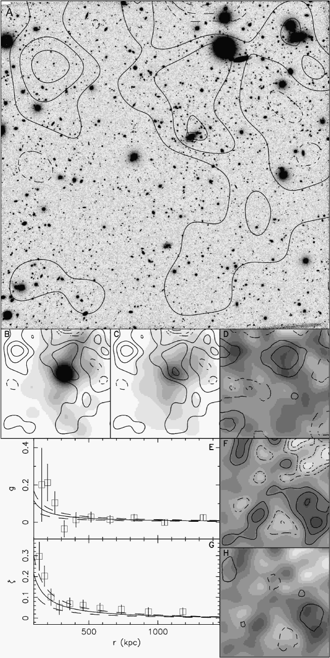
Figure 10: Shown in panels A–F are the figure for CLJ1411.1$-$1148, with images $6\aas@@fstack{\prime}99$ or 2.61 Mpc in the cluster restframe on a side, using the same layout as Fig. 2. The aperture densitometry significance contours of panels D and H use a $3\aas@@fstack{\prime}0$ aperture radius.

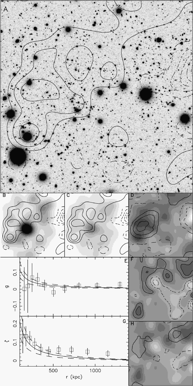
Figure 11: Shown in panels A–F are the figure for CLJ1420.3$-$1236, with images $6\aas@@fstack{\prime}6$ or 2.44 Mpc in the cluster restframe on a side, using the same layout as Fig. 2. The aperture densitometry significance contours of panels D and H use a $3\aas@@fstack{\prime}0$ aperture radius.

3 $z\sim 0.5$ Clusters

The weak lensing analyzes for the intermediate redshift sample are shown in Figs. 2–11, all of which have the same layout. The top panel (A) shows the $I$-band VLT image in greyscale overlayed with contours of the mass reconstruction. Each contour represents a change in the surface mass density of $10^{8}\mathrm{M}_{\odot}/\mathrm{kpc}^{2}$ relative to the mean surface mass at the edge of the image, with solid contours indicating a surface mass increase and dashed contours indicating a decrease. The mass reconstruction has been smoothed with a $25\aas@@fstack{\prime\prime}6$ circular Gaussian profile to remove high-frequency noise, which results in the cluster mass peaks having a broad core in the reconstruction even if the true mass profile has a cusp. As the edges of an image are located typically between 1000 kpc (nearest edge) and 1800 kpc (furthest corner) from the cluster core, the mean surface mass at the edge will still be significantly above the cosmic mean, and thus some of the negative mass contours may be real. The mass reconstructions are, to a good approximation, the sum of the true surface mass density field and a white-noise field resulting from the intrinsic ellipticities of the background galaxies. This noise field results not only in false mass peaks, but also in the displacement of true mass peaks, with less massive peaks suffering, on average, a greater displacement. Simulations have shown that a $5\sigma$ peak can be routinely displaced by up to $10\arcsec$ from its true position (Clowe et al. 2000). The chosen BCG for each cluster is indicated by a box drawn around it. In all of the figures north is up and east is to the left.

The middle left-hand panel (B) shows a luminosity map, also smoothed with a $25\aas@@fstack{\prime\prime}6$ circular Gaussian profile, of the photometric-redshift selected cluster galaxies in greyscale with the positive mass weak lensing reconstruction contours overlayed. The middle panel (C) shows a greyscale map of the number density of the cluster galaxies, again smoothed with a $25\aas@@fstack{\prime\prime}6$ circular Gaussian profile, with the positive mass weak lensing reconstruction contours overlayed. The greyscale for all of the clusters in panels B and C are identical except for CLJ1232.5$-$1250, which has the maximum of the scale extending to twice the values of the other clusters. The upper-middle right-hand panel (D) shows the mass reconstruction in greyscale with significance contours of the mass aperture statistic overlayed, with each contour indicating a significance step of $1\sigma$. The difference in positions of the reconstruction mass peaks and the mass aperture significance peaks are a result of the different weighting functions the two methods give to the shear field, and can be used as an estimate to the amount of error in the centroid positioning of the mass peaks due to noise. Using the mass aperture significance map to measure the significance of additional peaks results in a systematic overestimate of the peaks’ significance (van Waerbeke 2000) as what is being measured is the significance of the highest noise peak superimposed on the underlying mass distribution.

The two graphs show the reduced shear profile about the BCG (panel E) and the resulting aperture densitometry profile (panel G) as a function of radius from the BCG. Both graphs show the best fitting SIS profile (solid line) to the reduced shear profile and the $1\sigma$ errors (dashed lines).

The lower-middle right-hand panel (F) shows in both greyscale and contours, using the same contour levels as the mass reconstruction in the previous panels, the mass reconstruction of the field after rotating all of the background galaxies by 45 degrees. The mean shear profile of the cluster was first subtracted from the background galaxies’ shear measurements prior to the rotation. Because the weak lensing shear field is irrotational, the rotation of the background galaxies (equivalent to taking the curl of the shear field) produces an estimate of the noise in the reconstruction. The lower right-hand panel (H) has the same noise field in greyscale as panel F, but has the significance of the mass aperture statistic for the 45 degree rotated background galaxies overlayed in contours, with each contour indicating a significance step of $1\sigma$.

A summary of the weak lensing data for each cluster can be found in Table 2. A description of each cluster’s lensing analysis follows.

3.1 CLJ1018.8$-$1211

CLJ1018.8$-$1211 ($z=0.472$) is detected as a $\sigma_{\mathrm{v}}=603^{+82}_{-100}$ km/s cluster at moderate significance ($3.2\sigma$ in shear, $2.9\sigma$ in $M_{\mathrm{ap}}$). The offset observed between the BCG and the mass peak in the reconstruction is consistent with shifts of peaks due to noise with this significance. A second peak, with higher $\kappa$ but lower significance, is also detected in the south-west corner of the field. No spectra currently exist for this peak, but photometric redshifts indicate that is likely at a lower redshift and therefore unrelated to this cluster. The relatively high mass-to-light ratio of this cluster may indicate that the lensing mass includes some significant contribution from the lower redshift structure. The structure in the northwest corner in the mass reconstructions is detected at only $1\sigma$ in $M_{\mathrm{ap}}$, so is likely a noise peak.

3.2 CLJ1059.2$-$1253

CLJ1059.2$-$1253 ($z=0.457$) is the second most massive cluster in the sample, and the most massive in the intermediate redshift subsample, having a best fit SIS profile with $\sigma_{\mathrm{v}}=1033^{+69}_{-80}$ km/s and is detected at $5.8\sigma$ with the shear profile fitting and $4.7\sigma$ with $M_{\mathrm{ap}}$. The relatively low significance for the detection of a cluster of this mass is due to all three VLT passbands having higher than average seeing levels, and therefore having the lowest number density of background galaxies with which to measure the shear field. The $2\sigma$ peak located northwest of the cluster at the edge of the VLT field does not correspond to an overdensity of galaxies within the VLT image, but could, in theory, be caused by a structure immediately outside of the image.

3.3 CLJ1119.3$-$1129

No significant peaks are detected in this field. The shear profile about the BCG does indicate a positive mass, although only at $1.0\sigma$ significance. A $2\sigma$ upper limit on the velocity dispersion of the cluster is 600 km/s.

3.4 CLJ1202.7$-$1224

Several small peaks in this field exist in the mass reconstruction, the nearest of which is $\sim 1\aas@@fstack{\prime}5$ away from the likely BCG. In the $M_{\mathrm{ap}}$ map, however, a significant peak is located near this BCG, about $\sim 30\arcsec$ to the southeast. Using this galaxy ($z=0.424$) as the BCG gives a best fit SIS profile of $447^{+136}_{-214}$ km/s with a significance of $1.4\sigma$ from the shear profile and $1.5\sigma$ with $M_{\mathrm{ap}}$. Using a slightly fainter galaxy, located $28\arcsec$ south-east of the BCG, as the center of mass results in a best fit SIS profile of $570^{+120}_{-164}$ km/s with $2.0\sigma$ significance, $2.6\sigma$ significance with $M_{\mathrm{ap}}$. We do not have redshift information on this second galaxy, but photometric redshifts give it a high probability of being at the same redshift as the BCG. Several of the other peaks, none of which are significant at more than $1.3\sigma$, are also spatially coincident with red galaxy overdensities. The redshifts of these galaxy overdensities are not currently known, so it is uncertain if these smaller mass peaks are physically associated with the cluster.

3.5 CLJ1232.5$-$1250

CLJ1232.5-1250 ($z=0.542$) is the third most massive cluster in the sample, having a best fit SIS profile with $\sigma_{\mathrm{v}}=948^{+50}_{-51}$ km/s. The cluster is detected at $8.1\sigma$ significance with the shear profile and $7.1\sigma$ with $M_{\mathrm{ap}}$, which makes it the most significant lensing detection in the EDisCS sample. The mass peak, as one would expect for a peak with this high significance, is spatially coincident with the brightest cluster galaxy in both the mass reconstruction and $M_{\mathrm{ap}}$. There is a second mass peak in the south-west corner of the image which is also detected at more than $3\sigma$ significance and is near a group of red galaxies which have colors consistent with the cluster red-sequence. This secondary peak is the reason the filter radius for the highest significance $M_{\mathrm{ap}}$ statistic is smaller than most of the other clusters in the intermediate redshift sample. The larger radius would put this peak in the negative weight portion of the filter, and therefore decrease the significance of the cluster detection. As such, the $7.1\sigma$ significance is only a lower bound on the true significance of the cluster peak. The weak lensing mass measurement is in reasonable agreement with the $\sigma_{\mathrm{v}}=1080^{+119}_{-89}$ km/s velocity dispersion measured spectroscopically with 58 cluster galaxies (Halliday et al. 2004).

3.6 CLJ1238.5$-$1144

No significant peaks are detected in the mass reconstruction of this field. Using the likely BCG as the center of the shear profile gives a best-fit velocity dispersion of $\sigma_{\mathrm{v}}=375^{+138}_{-254}$ km/s and a significance of $1.1\sigma$ from the shear profile, but only a $0.4\sigma$ significance from $M_{\mathrm{ap}}$.

3.7 CLJ1301.7$-$1139

One massive peak, spatially coincident with several galaxy overdensities, is evident in the mass reconstruction shown in Fig. 8. At smaller smoothing radii, however, this peak breaks up into 3 peaks, each one located near one of the bright galaxies surrounding the peak shown in the figure. The southeast galaxy overdensity is the structure which was targeted by the observations and is a galaxy cluster at $z=0.48$. The northwest structure appears to be a second galaxy cluster at $z=0.39$, and it is currently unknown whether the middle structure is associated with one of these two clusters. These two clusters are too close in redshift to allow the photometric redshift measurements with our filter set to accurately determine to which cluster a given galaxy belongs, so the luminosity measurement can only be made for the sum of the two clusters. Using the BCG of the $z=0.48$ cluster as the center of the shear profile gives a best-fit velocity dispersion of $\sigma_{\mathrm{v}}=628^{+86}_{-104}$ km/s. This mass estimate, however, is certain to be contaminated with mass from the lower redshift cluster. The mass-to-light ratio for the system is consistent with the sample mean, as both the mass and luminosity measurements are being contaminated by the lower redshift cluster. Attempts to simultaneously fit both clusters result in a high degree of degeneracy between the two mass measurements.

3.8 CLJ1353.0$-$1137

A $\sigma_{\mathrm{v}}=546^{+130}_{-180}$ km/s peak, detected at $1.8\sigma$ significance in the shear profile and $1.4\sigma$ significance with $M_{\mathrm{ap}}$, is spatially coincident with the CLJ1353.0-1137 BCG ($z=0.577$). Another peak, with higher $\kappa$ but a lower significance, is located north-west of the cluster and between two galaxy overdensities. The southern-most of these galaxies overdensities has photometric redshifts consistent with the cluster, while the northern overdensity appears to be at lower redshift. The peak south-east of the cluster in the mass reconstruction is not spatially coincident with any galaxy overdensities. Neither of the additional peaks are significant in $M_{\mathrm{ap}}$ measurements.

3.9 CLJ1411.1$-$1148

A broad mass peak of low significance is detected at the location of the BCG ($z=0.520$). Using the BCG as the center of the peak gives a best fit SIS profile of $\sigma_{\mathrm{v}}=594^{+103}_{-128}$ km/s with a significance of $2.6\sigma$ from the shear profile and $1.4\sigma$ with $M_{\mathrm{ap}}$. The mass reconstruction shows evidence for long extensions to the south and west, although again at low significance. The extensions are not detected using $M_{\mathrm{ap}}$, although this is not unexpected as the cluster would be in the negative weight portion of the filter and therefore canceling any possible filamentary mass in the positive weight portion. Any filamentary mass will also be in the negative weight portion of the filter when centered on the cluster, which could explain the lower significance from $M_{\mathrm{ap}}$. An additional, low significance peaks are found in the north-east and south-east corners of the field, possibly associated with a lower-redshift galaxy overdensities found to near the peaks.

3.10 CLJ1420.3$-$1236

A broad mass peak is detected at moderate significance ($3.7\sigma$ from shear, $3.2\sigma$ from $M_{\mathrm{ap}}$) near CLJ1420.3$-$1236 ($z=0.497$). The offset between the centroid of the peak and the BCG is $\sim 50\arcsec$, which for a $4\sigma$ peak is significant at $\sim 3\sigma$. At smaller smoothing filters than that shown in Fig. 11, however, the peak breaks into two components, one of which is $\sim 20\arcsec$ from the BCG. The second component is not located near any significant concentration of galaxies. Using the BCG as the center of the cluster, one obtains a shear profile which is best fit by a $\sigma_{\mathrm{v}}=583^{+98}_{-118}$ km/s velocity dispersion and is significant at $2.7\sigma$ in the shear profile $1.8\sigma$ in $M_{\mathrm{ap}}$. Two additional peaks are located $\sim 1\aas@@fstack{\prime}5$ north-west and south-east of the cluster, both near galaxy overdensities which have the same photometric redshift as the cluster. The multiple peaks and the fact the reduced shear and aperture densitometry mass at large radius from the cluster core are much larger than the best fit SIS model predicts indicate that this is a massive cluster which is either just forming or undergoing one or more major mergers.

4 $z\sim 0.7$ Clusters

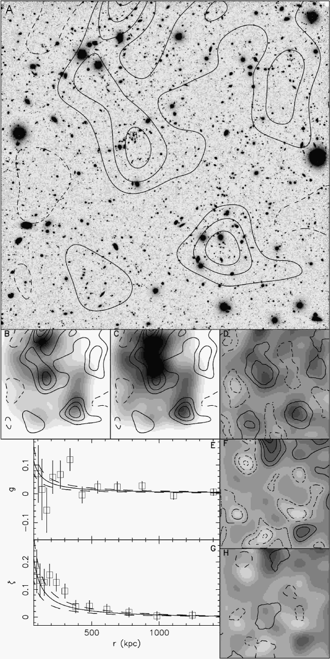
Figure 12: Shown in panels A–F are the figure for CLJ1037.9$-$1243, with images $6\aas@@fstack{\prime}80$ or 2.80 Mpc in the cluster restframe on a side, using the same layout as Fig. 2. The aperture densitometry significance contours of panels D and H use a $2\aas@@fstack{\prime}5$ aperture radius.

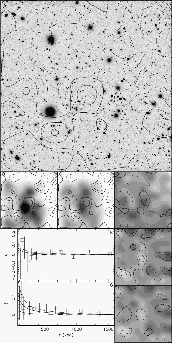
Figure 13: Shown in panels A–F are the figure for CLJ1040.7$-$1155, with images $7\aas@@fstack{\prime}15$ or 3.07 Mpc in the cluster restframe on a side, using the same layout as Fig. 2. The aperture densitometry significance contours of panels D and H use a $3\aas@@fstack{\prime}0$ aperture radius.

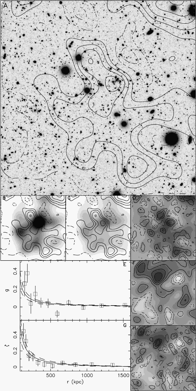
Figure 14: Shown in panels A–F are the figure for CLJ1054.4$-$1146, with images $7\aas@@fstack{\prime}09$ or 3.04 Mpc in the cluster restframe on a side, using the same layout as Fig. 2. The greyscale in panels B and C have their maximum value at twice that in Fig. 2. The aperture densitometry significance contours of panels D and H use a $1\aas@@fstack{\prime}0$ aperture radius.

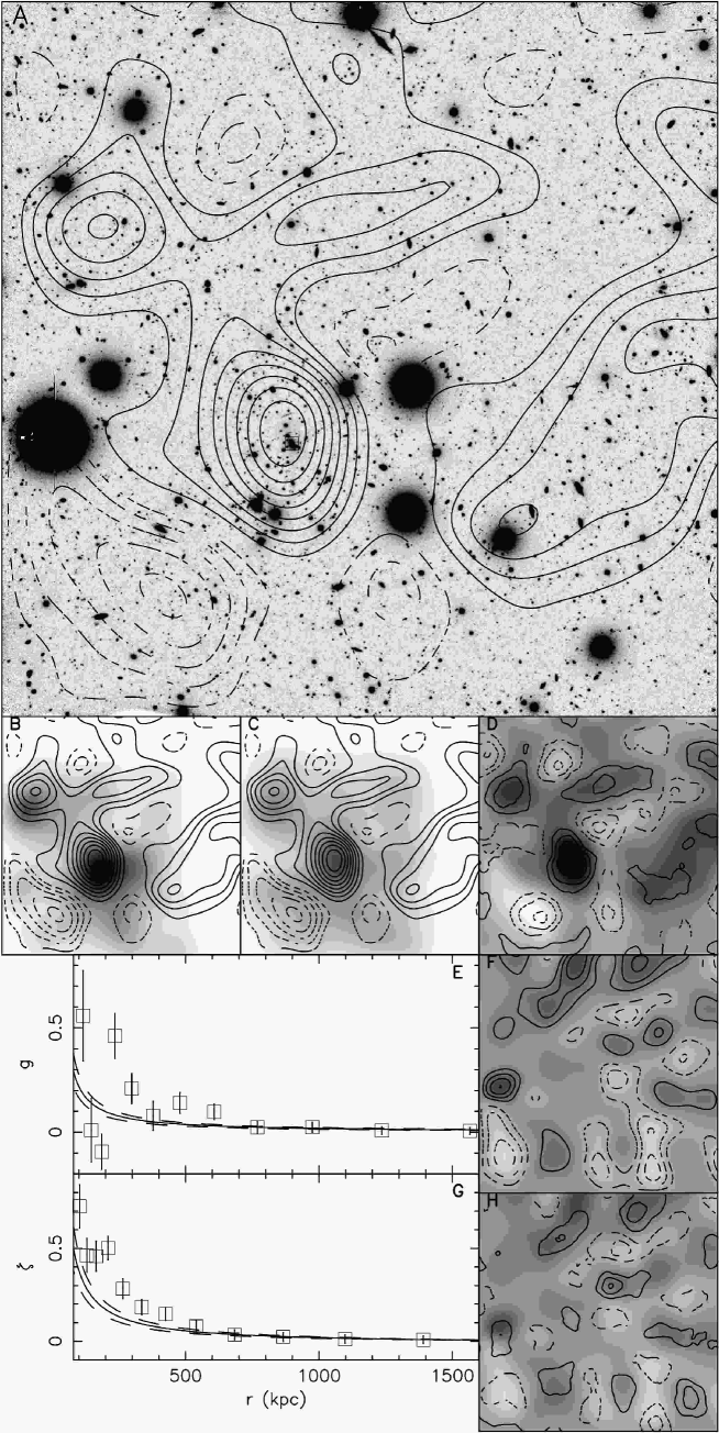
Figure 15: Shown in panels A–F are the figure for CLJ1054.7$-$1245, with images $7\aas@@fstack{\prime}04$ or 3.10 Mpc in the cluster restframe on a side, using the same layout as Fig. 2. The greyscale in panels B and C have their maximum value at twice that in Fig. 2. The aperture densitometry significance contours of panels D and H use a $1\aas@@fstack{\prime}5$ aperture radius.

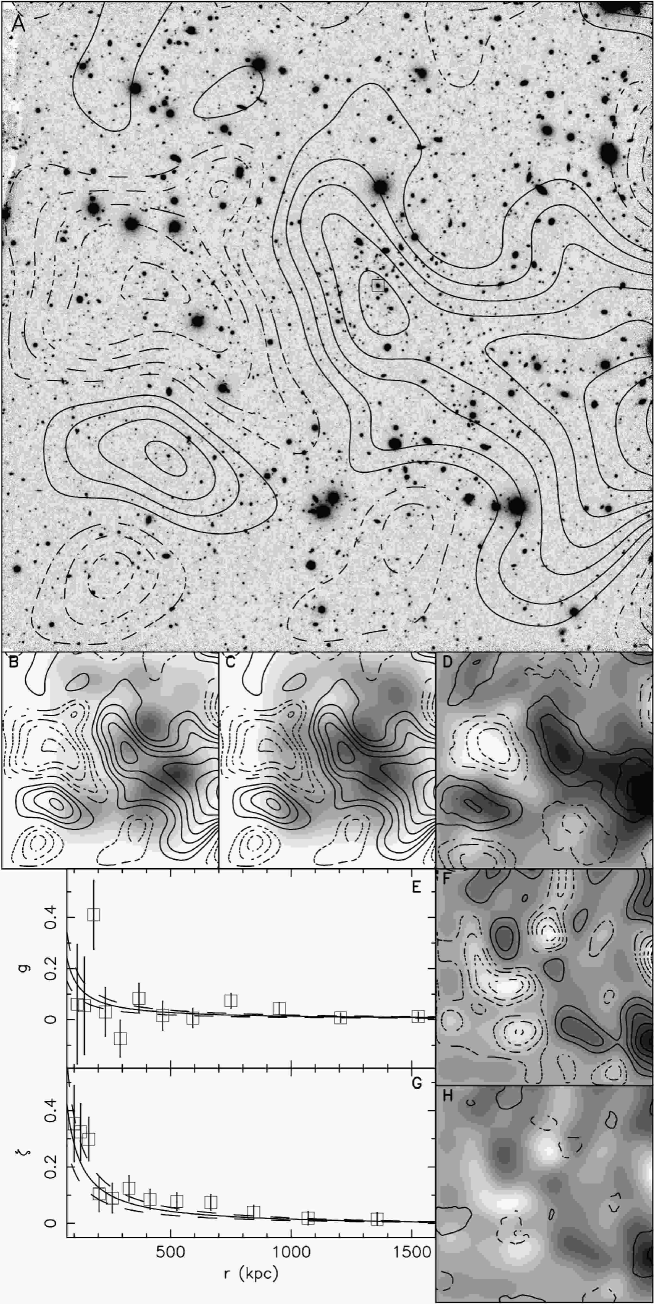
Figure 16: Shown in panels A–F are the figure for CLJ1103.7$-$1245, with images $7\aas@@fstack{\prime}15$ or 3.40 Mpc in the cluster restframe on a side, using the same layout as Fig. 2. The aperture densitometry significance contours of panels D and H use a $2\aas@@fstack{\prime}5$ aperture radius.

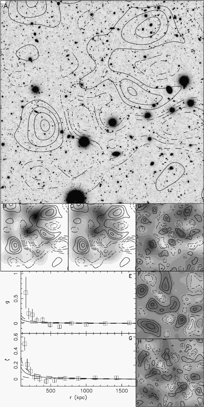
Figure 17: Shown in panels A–F are the figure for CLJ1122.9$-$1136, with images $7\aas@@fstack{\prime}09$ or 3.21 Mpc in the cluster restframe on a side, using the same layout as Fig. 2. The aperture densitometry significance contours of panels D and H use a $1\aas@@fstack{\prime}0$ aperture radius.

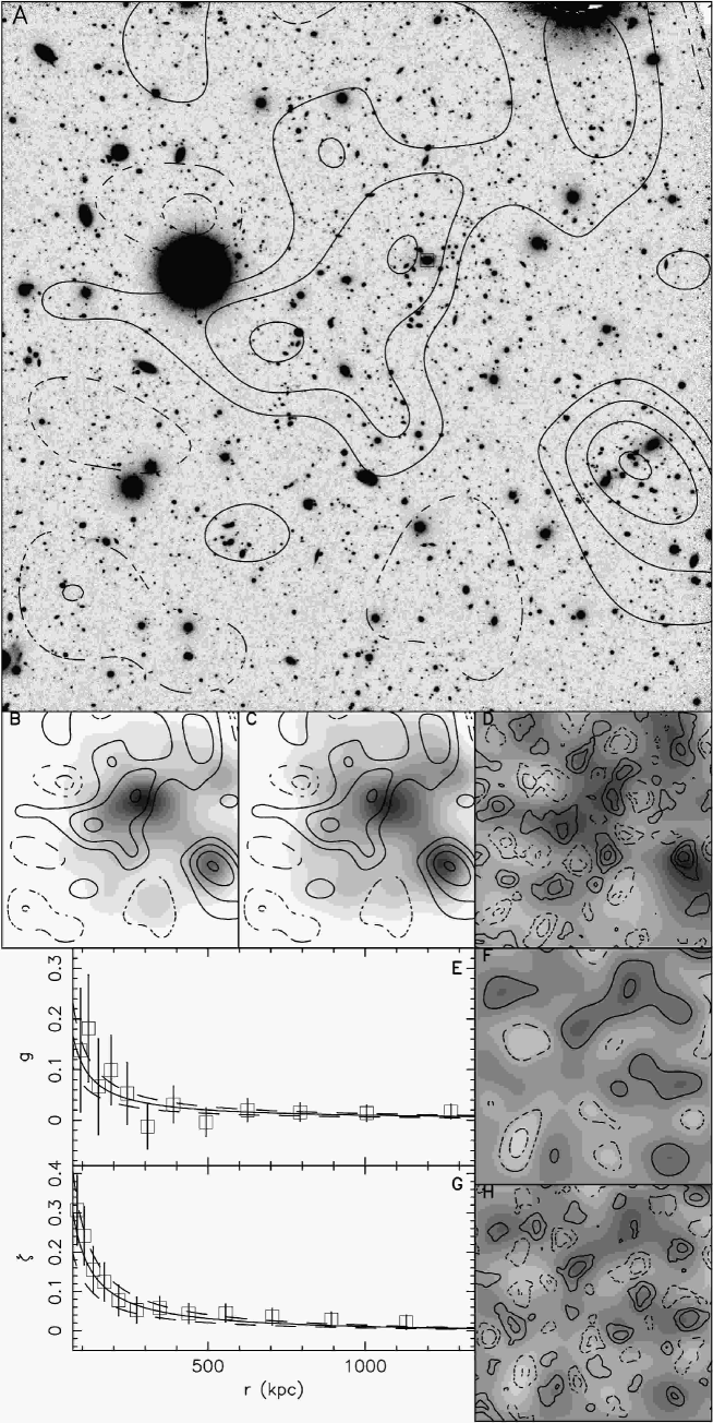
Figure 18: Shown in panels A–F are the figure for CLJ1138.2$-$1133, with images $7\aas@@fstack{\prime}04$ or 2.52 Mpc in the cluster restframe on a side, using the same layout as Fig. 2. The aperture densitometry significance contours of panels D and H use a $1\aas@@fstack{\prime}0$ aperture radius.

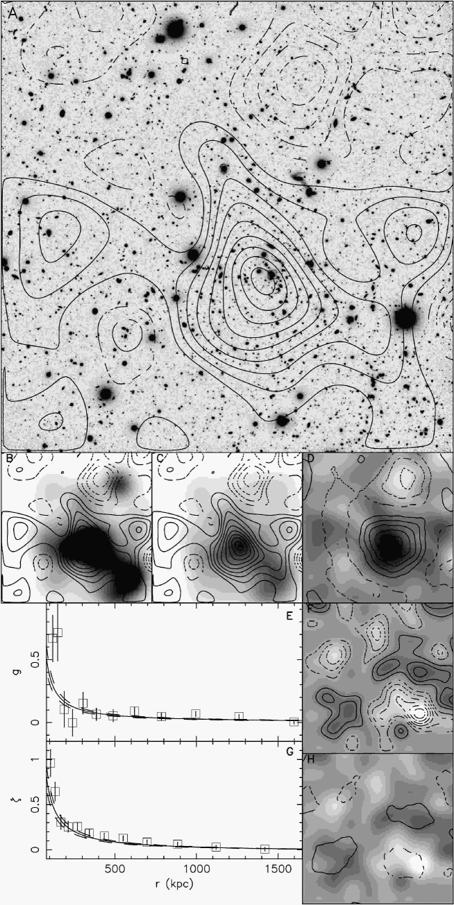
Figure 19: Shown in panels A–F are the figure for CLJ1216.8$-$1201, with images $7\aas@@fstack{\prime}09$ or 3.19 Mpc in the cluster restframe on a side, using the same layout as Fig. 2. The greyscale in panels B and C have their maximum value at twice that in Fig. 2. The aperture densitometry significance contours of panels D and H use a $3\aas@@fstack{\prime}0$ aperture radius.

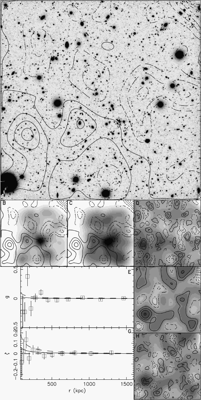
Figure 20: Shown in panels A–F are the figure for CLJ1227.9$-$1238, with images $7\aas@@fstack{\prime}15$ or 2.94 Mpc in the cluster restframe on a side, using the same layout as Fig. 2. The aperture densitometry significance contours of panels D and H use a $1\aas@@fstack{\prime}5$ aperture radius.

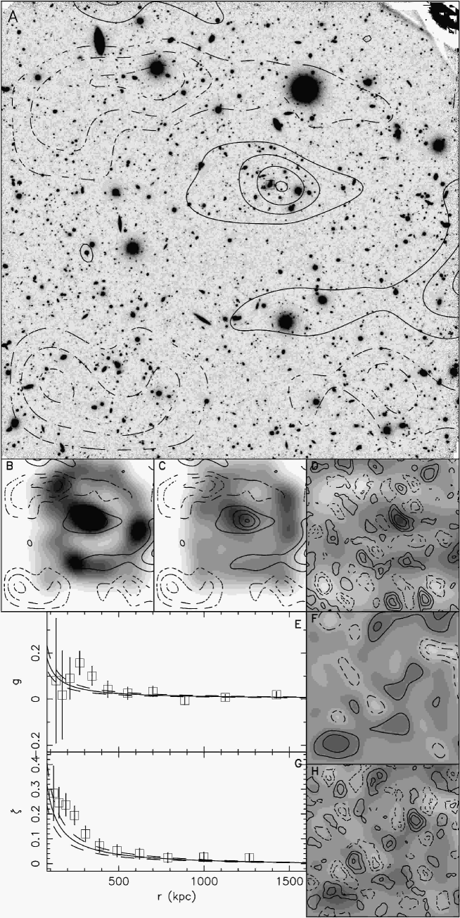
Figure 21: Shown in panels A–F are the figure for CLJ1354.2$-$1230, with images $7\aas@@fstack{\prime}15$ or 3.16 Mpc in the cluster restframe on a side, using the same layout as Fig. 2. The aperture densitometry significance contours of panels D and H use a $1\aas@@fstack{\prime}0$ aperture radius.

The weak lensing results for the high-redshift sample are shown in Figs 12–21, using the same layout as the intermediate redshift sample. The greyscale range in panels B and C are the same as for the intermediate redshift sample except for CLJ1054.4$-$1146, CLJ1054.7$-$1245, and CLJ1216.8$-$1201, which have the maximum in the scale range at twice the normal value. A summary of the weak lensing data for each cluster can be found in Table 3. A description of each cluster’s lensing analysis follows.

4.1 CLJ1037.9$-$1243

In this field are two clusters, a $z=0.580$ cluster located slightly north-east of the center of the field and a $z=0.43$ cluster located in the southwest portion of the field. Both clusters are detected in the weak lensing reconstruction at moderate significance. The north-eastern cluster, which is the one identified in the LCDCS as being at high-redshift, is best fit with a $\sigma_{\mathrm{v}}=503^{+84}_{-102}$ km/s SIS model and is detected at a $2.7\sigma$ significance in the shear profile and $3.0\sigma$ with $M_{\mathrm{ap}}$. The south-western cluster is best fit with a $\sigma_{\mathrm{v}}=513^{+61}_{-72}$ km/s SIS model and is detected at a $3.7\sigma$ significance in the shear profile and $2.8\sigma$ with $M_{\mathrm{ap}}$. Both of these mass measurements are presumably biased toward higher masses by the other peaks. Attempts at fitting both peaks simultaneously results in a large covariance between the two peaks, due mainly to the small field size not providing a good constraint on the total mass. Additionally, in the lensing reconstruction is a northern extension from the north-eastern cluster which continues until the edge of the image. This northern extension is also found in the cluster galaxy distribution. The sharp rise in the surface mass density in the reconstruction at the northern edge of this extension is not found in the mass aperture significance map, and is likely due to the increased noise level at the edges of the reconstruction.

4.2 CLJ1040.7$-$1155

No significant peaks are detected in this field. Using the BCG as the center of the cluster we find a best-fit mass model which has positive mass, but is significant only at $1.3\sigma$ in shear and $1.0\sigma$ with $M_{\mathrm{ap}}$. The $2\sigma$ upper limit on the velocity dispersion for this cluster is 684 km/s. The weak lensing mass measurement is in good agreement with the $\sigma_{\mathrm{v}}=418^{+55}_{-46}$ km/s velocity dispersion measured from spectra of 30 cluster members (Halliday et al. 2004).

4.3 CLJ1054.4$-$1146

A $\sigma_{\mathrm{v}}=885^{+99}_{-117}$ km/s mass peak is detected near the BCG of CLJ1054$-$1146 ($z=0.697$) at $3.8\sigma$ significance in shear and $2.9\sigma$ with $M_{\mathrm{ap}}$. Additional peaks are found $3\arcmin$ south-southwest of the cluster, $3\arcmin$ south-southeast of the cluster, $1\aas@@fstack{\prime}5$ east-southeast of the cluster, and $1\arcmin$ northeast of the cluster. The SSW cluster is detected at the $2.4\sigma$ level with $M_{\mathrm{ap}}$, the other three at $\sim 2\sigma$. The SSW peak is located near a galaxy group with photometric redshifts of 0.25, while the two southeastern peaks are located near large, unconcentrated galaxy overdensities with photometric redshifts consistent with cluster galaxies. The northwestern peak does not have any galaxy overdensities nearby. In addition, there is a long filamentary like extension starting $\sim 1\arcmin$ south of the cluster and running due west, which overlaps two galaxy overdensities, one of which is likely to be around $0.8<z<1.0$ while the other is at lower redshift than the cluster, from the photometric redshifts. The weak lensing mass measurement is much larger than the $\sigma_{\mathrm{v}}=589^{+78}_{-70}$ km/s velocity dispersion measured from spectra of 48 cluster members (Halliday et al. 2004). This mass discrepancy, combined with the large swath of similar redshift galaxies to the east of the cluster and that the mass-to-light ratio from the weak lensing mass measurements are consistent with the sample average, suggests that a large amount of mass is currently infalling into the cluster. Such mass would be included in the weak lensing estimates but would not have yet affected the velocity dispersion of the cluster galaxies. A large, diffuse screen of mass would also explain why the $M_{\mathrm{ap}}$ significance is lower than that from the shear profile and why the highest $M_{\mathrm{ap}}$ significance is from the smallest filter radius used.

4.4 CLJ1054.7$-$1245

CLJ1054$-$1245 ($z=0.750$) is detected as the fourth most massive cluster in the EDisCS sample, with a $\sigma_{\mathrm{v}}=906^{+88}_{-102}$ km/s velocity dispersion at $4.4\sigma$ significance in shear and $4.9\sigma$ with $M_{\mathrm{ap}}$. Three additional, less significant peaks are located $\sim 2\arcmin$ west, north and northeast of the cluster. The northeastern peak is located near an overdensity of galaxies with photometric redshifts of $\sim 0.6-0.66$. The western peak is located near an overdensity of lower redshift galaxies, while the northern peak is not obviously associated with any large galaxy grouping. The weak lensing cluster mass is much larger than the spectroscopic velocity dispersion $\sigma_{\mathrm{v}}=504^{+113}_{-65}$ km/s (Halliday et al. 2004). One possible explanation for the discrepancy would be that the cluster has a triaxial mass distribution with a dominant major axis, and that this axis is closely aligned to the line-of-sight through the cluster. This would result in a large amount of mass being projected into a small area centered on the cluster BCG, and produce an overestimate of the central density of the cluster in the weak lensing mass measurements. Such alignments in simulated clusters result in large overestimates of the dynamical mass of the cluster (Clowe et al. 2004a). Another possible explanation stems from the spectroscopic survey, which shows that this cluster may have an extended tail toward high-redshift, and that many of these galaxies in this high-redshift tail are spatially coincident in projection with the cluster core. This may indicate an extended filamentary structure along the line-of-sight associated with the cluster, with the weak lensing observations including all of the mass of the filament. The mass-to-light ratio of the cluster, however, is consistent with the sample average, suggesting that the high weak lensing mass is not an overestimate due to noise. Using the velocity dispersion of the cluster galaxies to calculate the mass, results in a mass-to-light ratio which is significantly lower than the sample average. There are also two probable strong lensing giant arcs in the cluster, both located north of the BCG. The brighter of these two is at a distance of $17\arcsec$ from the BCG, which is consistent with the weak lensing mass measurement if this galaxy is at $z\sim 1.5$. We do not have a spectroscopic redshift for this arc, but photometric redshifts give it a best-fit redshift of 1.7, with an allowable range of 1.2 to 1.8.

4.5 CLJ1103.7$-$1245

At $z=0.96$, CLJ1103.7$-$1245 is the highest redshift cluster in the EDisCS sample. Using the chosen BCG as the mass centroid results in a moderately significant mass peak ($3.0\sigma$ in shear and $2.9\sigma$ with $M_{\mathrm{ap}}$). Spectroscopy has shown, however, that there are two additional galaxy concentrations near this cluster, one to the southwest of the cluster at $z=0.63$ and one to the northwest at $z=0.70$. The $z=0.70$ structure is not detected in the weak lensing mass reconstruction, while the $z=0.63$ structure is likely responsible for the large $\kappa$ peak at the western edge of the mass reconstruction. Even though the $z=0.63$ structure has a much larger $\kappa$ value in the reconstruction, due to the difference in $\Sigma_{\mathrm{crit}}$ the $z=0.96$ cluster is the most massive structure in the reconstruction. The measured mass for the cluster, however, is likely overestimated due to the inclusion of the surface densities of the other two structures in the radial shear measurements, as can be seen by the bump in $\kappa$ from the aperture densitometry measurements in panel G of Fig. 16 between 400 and 700 kpc (which is the separation between the cluster and the $z=0.63$ structure). The extremely high mass-to-light ratio measured for this cluster is likely due in part to the overestimation of the mass due to the projected structures and an underestimation of the total light, as compared to the lower redshift clusters, due to the incompleteness limit in the luminosity profile occurring at a brighter absolute magnitude. It should also be noted that the $z=0.96$ cluster is also being lensed by the $z=0.63$ structure, which will result in it being displaced by a few arcseconds from its true position and a magnification of the cluster galaxies by $\sim 0.1$ magnitudes.

4.6 CLJ1122.9$-$1136

No significant peaks are detected in this field. Using the brightest galaxy in a small group near where the LCDCS peak is located gives a best-fit $\sigma_{\mathrm{v}}=589^{+172}_{-262}$ km/s SIS profile at $1.4\sigma$ significance in shear and $2.3\sigma$ with $M_{\mathrm{ap}}$.

4.7 CLJ1138.2$-$1133

A moderately significant mass peak is located near the BCG of CLJ1138$-$1133 ($z=0.480$) with $\sigma_{\mathrm{v}}=529^{+78}_{-96}$ km/s velocity dispersion at $2.9\sigma$ significance in shear and $1.4\sigma$ with $M_{\mathrm{ap}}$. Two additional, smaller peaks are located $1\aas@@fstack{\prime}5$ northeast and $2\arcmin$ southeast of the cluster, both near galaxy overdensities of similar redshift to the cluster. Another more significant peak is located $4\arcmin$ southwest of the cluster and is spatially coincident with an overdensity of lower redshift galaxies. The two peaks near the cluster are likely the result of the small filter radius for the highest significance $M_{\mathrm{ap}}$ measurement and its lower significance compared to that of the shear profile. The mass of these two peaks are included in the total mass of the system at radii larger than their separation from the cluster core.

4.8 CLJ1216.8$-$1201

CLJ1216-1201 ($z=0.794$) is the most massive cluster in the EDisCS sample, with a best-fit SIS model with $\sigma_{\mathrm{v}}=1152^{+70}_{-78}$ km/s and a $6.8\sigma$ significance in the shear profile and $5.2\sigma$ with $M_{\mathrm{ap}}$. A three-image, strong lensing arc system is also located in the cluster at a $\sim 15\arcsec$ radius from the BCG. The weak lensing mass is in reasonable agreement with the $\sigma_{\mathrm{v}}=1018^{73}_{-77}$ km/s velocity dispersion measured from spectra of 67 cluster members (Halliday et al. 2004). The cluster galaxies have a northern and south-western filamentary-like extension, both of which are detected at moderate significance in the mass reconstruction. The mass from these filaments would be located in the negative weight portion of the $M_{\mathrm{ap}}$ filter, which would explain the lower significance compared to the shear profile.

4.9 CLJ1227.9$-$1138

A marginally significant mass peak is located in this field, with $2.3\sigma$ significance in shear and $1.8\sigma$ significance with $M_{\mathrm{ap}}$, but is $1\aas@@fstack{\prime}5$ displaced from the BCG of CLJ1227.9$-$1138 ($z=0.634$). The peak does not appear to be associated with any overdensity of galaxies (the bright, extended object near the center of the peak in Fig 20 is is actually two blended stars). Using the BCG as the center of a shear profile results in a best-fit SIS model with $\sigma_{\mathrm{v}}=308^{+221}_{-308}$ km/s at a $0.5\sigma$ significance in the shear and $1.2\sigma$ significance with $M_{\mathrm{ap}}$. The $2\sigma$ upper limit on the velocity dispersion is 600 km/s.

4.10 CLJ1354.2$-$1230

A moderately significant mass peak is located near the BCG of CLJ1354.2$-$1230 ($z=0.598$) with a $\sigma_{\mathrm{v}}=747^{+87}_{-98}$ km/s velocity dispersion at $3.9\sigma$ significance in shear and $3.7\sigma$ with $M_{\mathrm{ap}}$. The broad, filamentary-like structure seen in the mass reconstruction south of the cluster breaks up into several $2\sigma$ peaks in $M_{\mathrm{ap}}$ measurements, and is located near a small group of lower redshift galaxies.

5 Discussion

Figure 22: Plotted above are the best-fit SIS velocity dispersions for the EDisCS clusters (stars), high-$z$ X-ray selected clusters from Clowe et al. (2000) (squares), and lower redshift X-ray selected cluster samples from Dahle et al. (2002) (circles) and Cypriano et al. (2004) (triangles). The error bars for the EDisCS and high-$z$ X-ray selected samples are given as $1\sigma$, but the measured quantity is proportional to the square of the velocity dispersion. The lines show a model for the evolution of the cluster mass with redshift from Wechsler et al. (2002).

Because the mass reconstructions are the combination of the true mass surface density field and a noise field, the position and shape of the cluster mass peak can be greatly altered by the noise field. As such, if one were to pick the centroid of the mass peak in the 2-D reconstruction as the center of mass of the cluster, the resulting best-fit mass profile would tend to overestimate the cluster mass as one is picking the highest noise peak which is near the true mass peak. We have instead assumed that the BCG is the center of cluster for making the mass and significance measurements in Tables 3 and 2. For relaxed clusters, N-body simulations suggest that the BCG is a good choice for the center of the cluster (Frenk et al. 1996). Because these clusters are located in the epoch of massive cluster formation (eg. Eke et al. 1996), however, there is a strong likelihood that many of the clusters are undergoing a major merger event and that the BCG may not be located at the center of mass of the cluster. For such cases we will be underestimating the true mass and significance of the cluster.

While only eight of the twenty clusters are detected at greater than $3\sigma$ significance, all of the clusters are detected with a best-fitting mass model which has positive mass (positive $\sigma^{2}$ in the SIS fits). If there was not a large mass concentration associated with the clusters then half of the clusters, on average, would be detected with best-fitting mass models which have negative mass. Thus, while we cannot conclude with any confidence that the seven clusters which we detect at less than $2\sigma$ significance (CLJ1119.3$-$1129, CLJ1202.7$-$1224, CLJ1238.5$-$1144, CLJ1353.0$-$1137, CLJ1040.7$-$1155, CLJ1122.9$-$1136, and CLJ1227.9$-$1138) individually have an associated mass overdensity, collectively we measure a $3\sigma$ significance that, on average, these clusters have mass associated with them. This significance was calculated both from the probability that a Gaussian error function on a zero mass model would produce seven positive mass measurements at or greater than the measured significances, and from stacking the background galaxy catalogs of the seven clusters after aligning to a common BCG position and measuring the significance of the resulting best-fit mass model.

We show in Figure 22 the best-fit SIS velocity dispersions for the EDisCS clusters, along with the high-$z$, X-ray selected clusters of Clowe et al. (2000) and lower redshift samples of Dahle et al. (2002) and Cypriano et al. (2004). Also shown are models for the mass growth rate of clusters from Wechsler et al. (2002). In these models, the clusters grow as $\propto\exp(-\alpha z)$, with massive clusters having typical $\alpha$ values measured in simulations between 1.1 and 1.6. The plotted lines assume a value of $\alpha=1.4$, which indicates a formation redshift of $z\sim 1.05$ (van den Bosch 2002). The change in the measured velocity dispersion was calculated by converting the cluster mass into a characteristic radius and concentration via the equations in Navarro et al. (1997). These were then used to calculate the reduced shear profile for the cluster, which was then fit over the same radial range as the measured data with a projected SIS model. The two lower redshift samples were selected to have high X-ray luminosity, and are representative of the most massive clusters in the nearby, $0.1\ga z\la 0.3$, universe. The total sky area covered by the X-ray surveys which found the high-$z$ clusters shown in Figure 22 is $\sim 200\Box^{\circ}$ (Henry et al. 1992, 2001), or roughly 1.5 times that of the LCDCS. As a result, we would expect to find in EDisCS on order of 2 clusters of mass comparable to the X-ray selected clusters in each of the two redshift groupings of the sample. There are two clusters in the $z\sim 0.5$ sample and one in the $z>0.6$ sample which have measured masses comparable with the X-ray selected clusters, in statistical agreement with expectations.

As can be seen in Figure 22, the X-ray selected, high-$z$ clusters are only comparable with the highest mass tip of the lower redshift cluster mass distribution. The EDisCS clusters are more comparable in mass range to the lower redshift distribution, but do have a bias toward finding higher mass clusters at higher redshift. The mass comparison with the lower redshift clusters, however, do come with a number of caveats. First, the Wechsler et al. (2002) models were only measured for clusters with $z=0$ masses of up to $10^{15}M_{\odot}$, while the $z=0$ masses for many of the EDisCS clusters from these models will wind up being several times that. Second, the plotted velocity dispersions are measured by fitting the azimuthally-averaged shear profiles around the cluster centers with a projected spherical SIS shear profile, but as the area on the sky observed around both sets of clusters was of similar size, the fit for the EDisCS clusters goes out to much larger radius than that of the lower redshift sample. As SIS models are known not to provide a good fit to clusters at large radii (Clowe & Schneider 2001, 2002), the differing scales for the fits may provide a bias which is dependent on the redshift of the cluster.

The significance of the secondary peaks in the mass reconstructions is best determined with the $M_{\mathrm{ap}}$ statistic, which, because it is a compensated filter, is relatively insensitive to the presence of the cluster in the field provided the cluster mass centroid is not within the aperture. The mass aperture statistic has been shown to have Gaussian errors regardless of the ellipticity distribution of the background galaxies (Schneider 1996), and has the property that moving the center of the aperture by half of a filter radius results in a mass measurement which is uncorrelated with the previous peak. Like the mass reconstructions, however, the mass aperture statistic is a combination of the true signal and a noise field, so simply looking for peaks in an oversampled map, such as that shown in panels d and h in Figs. 2–21, will result in peaks being measured as more significant they they truly are on average. Instead, to obtain an unbiased measurement of the structure’s $M_{\mathrm{ap}}$ value and significance, one must obtain an independent measurement of the position of the center of mass for the structure. One can, however, make a statistical measurement of the amount of structure in a given field using a grid of $M_{\mathrm{ap}}$ measurements, with each measurement point separated from the others by at least half the filter radius.

We constructed $M_{\mathrm{ap}}$ grids using the filter radii given in Tables 2 and 3 for each cluster, positioning the grid such that one point was placed on the centroid of the BCG. We then excluded that point and the 12 nearest points (those which had the BCG within the radius of the $M_{\mathrm{ap}}$ filter) from the measurements and counted the number of grid points which had $M_{\mathrm{ap}}$ significances of greater than $2\sigma$. For a $7\arcmin\times 7\arcmin$ field one would expect to find, on average, 0.69, 1.0, 1.56, 2.77, and 6.23 positive $M_{\mathrm{ap}}$ values with greater than $2\sigma$ significance using $3\aas@@fstack{\prime}0,2\aas@@fstack{\prime}5,2\aas@@fstack{\prime}0,1\aas@@fstack{\prime}5,$ and $1\aas@@fstack{\prime}0$ filter radii respectively. On average, we find each field has 1.7 times the number of $2\sigma$ or greater significance values than expected from the noise in the $M_{\mathrm{ap}}$ maps, suggesting that $\sim 60\%$ of the points are due to noise and the other $\sim 40\%$ are real mass structures along the line of sight. There are four times as many $3\sigma$ or greater significance points which are not spatially coincident with the cluster as would be expected from noise, suggesting that $\sim 75\%$ of these are real mass overdensities. Only one of these $3\sigma$ mass points, in CL1420.3$-$1236, is not spatially coincident with a galaxy overdensity. It should be noted, however, that this method will overestimate the number of detected points at a given significance level as compared to a noise-free model of a given power spectrum due to more low-mass peaks being scattered to higher significance than high mass peaks being scattered to lower significance. As such, any comparison of such counts with models will need to accurately model the noise properties of the data.

The weighted mean mass-to-light ratio over the sample is $133\pm 35\mathrm{M}_{\odot}/\mathrm{L}_{\odot}$ in rest-frame $I$ and $175\pm 46\mathrm{M}_{\odot}/\mathrm{L}_{\odot}$ in rest-frame B. Two clusters, CL1040.7$-$1155 and CL1227.9$-$1148, have mass-to-light ratios (in both passbands) which are more than $1\sigma$ below the mean. Three clusters have mass-to-light ratios that are more than $1\sigma$ above the mean. Two of these clusters (CL1059.2$-$1253 and CL1103.7$-$1245), however, have additional mass peaks which are likely associated with galaxy overdensities at different redshifts from the cluster. The weak lensing mass for these clusters likely has some contribution from these additional structures, while the photometric redshift selection of cluster galaxies excludes these additional overdensities from the cluster luminosity measurement. Five additional clusters have secondary mass peaks from structures unlikely to be associated with the clusters which are close enough to affect the weak lensing mass measurements, CL1018.8$-$1211, CL1037.9$-$1243, CL1138.2$-$1133, CL1301.7$-$1139, and CL1354.2$-$1230. For CL1301.7$-$1139, the secondary structure is close enough in redshift to the cluster that the photometric redshifts cannot distinguish between the two, so both the mass and luminosity measurements are contaminated by the structure, resulting in a mass-to-light ratio which is consistent with the sample mean. CL1018.8$-$1211, CL1039.9$-$1245, and CL1138.2$-$1133 have mass-to-light ratios which are more than $0.5\sigma$ higher than the sample mean. When we exclude the seven clusters that are likely contaminated by projected structures, the mean mass-to-light ratio for the sample becomes $121\pm 31\mathrm{M}_{\odot}/\mathrm{L}_{\odot}$ in $I$ and $162\pm 42\mathrm{M}_{\odot}/\mathrm{L}_{\odot}$ in $B$.

Figure 23: Plotted above are the best-fit SIS velocity dispersions for the EDisCS clusters versus the significance of the mass aperture detection. The solid stars show the results for the 7 clusters with additional, unrelated mass peaks near enough to the cluster to potentially bias the velocity dispersion measurements. The open boxes show the results for the other 13 clusters in the sample.

Fitting the mass-to-light ratio as a bi-linear function of redshift and velocity dispersion squared gives a best fit model, taking into account the high degree of correlation in the errors of the mass-to-light ratio and velocity dispersion squared, of

$${M\over L_{I}}=310^{+85}_{-90}-280^{+120}_{-140}\ z+\left(0.8^{+1.6}_{-2.0}\right)\times 10^{-5}\ V^{2}$$ (10)

for restframe $I$ and

$${M\over L_{B}}=480^{+95}_{-160}-460^{+130}_{-240}\ z+\left(0.4^{+1.7}_{-2.4}\right)\times 10^{-5}\ V^{2}$$ (11)

for restframe $B$. The errors for each fit parameter were measured by marginalizing over the other two fit parameters, are quoted for $68\%$ confidence limits but are not Gaussian, and there is a large anti-correlation between the intercept and the redshift dependent slope which keeps the mass-to-light ratio at $z\sim 0.6$ relatively constant. For both passbands we measure a mass-normalized brightening of the clusters at $98.4\%$ and $97.6\%$ significance for $I$ and $B$ bands respectively with increased redshift. The amount of brightening observed is broadly consistent with passive evolution models with starbursts at $z\sim 3-4$ for cluster galaxies (e.g. Bruzual & Charlot 2003). We note, however, that there are several potential systematic errors in this measurement: First, because of the different passbands observed in the two redshift samples, any biases in the photometric redshift selection of cluster galaxies are likely to also be different in the two samples. Both samples, however, have had the photometric redshifts checked with spectroscopic redshifts and no significant difference in selection biases have been found (Pello et al. 2004). Second, because the mass and luminosity have been corrected by subtraction of an outer annular measurement of a fixed size on the sky, the physical scale of this subtracted region varies with cluster redshift. As a result, if there is a change in the cluster mass-to-light ratio with radial distance from the cluster center, then these corrections could cause a bias in the measurement. Finally, the fits are dominated by the most massive cluster (CL1216.8$-$1201 at $z=0.794$); the removal of this cluster from the sample decreases the slope by $\sim 15\%$ in both passbands and the significance to $90\%$ and $88\%$ for $I$ and $B$ bands.

We show in Figure 23 the relation between the significance in the mass aperture statistic and the best fit SIS model’s velocity dispersion for each cluster. As one would expect due to both statistics being measured from the shear, there is a strong correlation between the two measurements. There is not, however, a clear distinction in the relation between the 7 clusters with nearby unrelated mass peaks and the other 13 clusters in the sample. This suggests that cluster catalogs selected using the mass aperture statistic will likely face a similar level of contamination by projected structures as optically selected catalogs. There is no significant correlation between the mass-to-light ratio and the mass aperture significance, so such a catalog would not be biased towards low mass-to-light ratio clusters, as an optically selected cluster conceivably could be.

5.1 Summary

We present weak gravitational lensing mass reconstructions for the 20 clusters in the ESO Distant Cluster Survey. We show that the clusters span a large range in mass, with the most massive clusters having a number density on the sky consistent with similar redshift clusters found in X-ray surveys and the overall mass range similar to that found among luminous X-ray clusters at low ($z\la 0.3$) redshifts. We find that 7 of the 20 clusters have additional, unrelated structures along the line of sight which are massive enough to be detected in the mass reconstructions and are likely to contaminate the lensing mass measurements for the clusters. The additional structures, however, are unlikely to have affected the cluster detection method of the LCDCS as they are typically much further from the cluster than the smoothing kernel used to detect the cluster light. We detect a positive mass for all 20 clusters, although 7 of these are detected at less than $2\sigma$ significance. We argue that the lack of any best-fitting models with negative mass indicates that these poorer clusters still have a significant amount of mass associated with them and are not projections of unrelated galaxies along the line of sight.

We use photometric redshifts to select likely cluster galaxies and measure the cluster luminosity within the central 500 kpc radius. We calculate a mass-to-light ratio for the cluster in both restframe $I$ and $B$ passbands, and find that the clusters with the additional structures superimposed on the cluster do, on average, have a higher measured mass-to-light ratio. For the remaining 13 clusters, we find that the clusters tend to have a lower mass-to-light ratio at higher redshift, but find no change in the mass-to-light ratio with cluster mass.

Appendix A Background galaxy number counts and shear noise-levels

Figure 24: Plotted above are the number density of background galaxies usable for shear measurements (top panels) and the rms shear noise-level per sq. arcminute per shear component from these galaxies (bottom panels) as a function of PSF size for the four observed passbands ($I,R,V,$ and $B$) and the combined catalog ($T$). The 2-hour exposure time images of the high-$z$ clusters are plotted as squares, while the 45-minute exposure time images of the lower redshift clusters are plotted as circles.

Because the optical images used in this analysis were all taken with the same telescope and instrument over a relatively short period of time using the same observing strategy, the variation in the number density of faint, background galaxies and their rms shear measurements between the fields should be mostly a function of PSF size, exposure time, bandpass, and cosmic variance without any systematic errors from varying telescope and camera optics. As such, this data set provides an excellent database to study the effects that the various observing conditions can have on expected noise levels in future ground–based surveys.

In Tables 2 and 3 we give the number density of background galaxies rms shear variance in the final galaxy catalog used for the cluster mass reconstructions. In Figure 24 we show the number density of background galaxies and a shear-field noise estimate (as rms shear per sq. arcmin per shear component) as a function of PSF FWHM for each observed passband and the combined catalog. In order to calculate the rms shear variation for the galaxies, we first subtracted a smoothed shear-field, using a $10\arcsec$ Gaussian smoothing kernel, from each galaxies shear measurement as a first-order correction to remove the cluster shear signal which would otherwise cause the fields around higher-mass clusters to be detected as having a higher noise level.

As can be seen, in general the deeper 2–hour exposures do provide a small increase in the number density of background galaxies over the 45–minute exposures with similar PSF FWHM. Reducing the size of the PSF, however, results in a much larger increase in the number density of usable background galaxies, with $0\aas@@fstack{\prime\prime}6$ FWHM, 45-minute exposure time images having the same or more usable background galaxies than $0\aas@@fstack{\prime\prime}7$ FWHM, 2-hour exposure time images. Further, the longer exposure time images have the greatest advantage over the shorter exposure image images at the smallest PSF levels. The exception is in the $I$-band, where the longer exposure images have similar numbers of background galaxies as the shorter. This appears to be due to three factors: First, the initial galaxy catalogs were created from a combined image in which all of the passbands were coadded using the inverse of the square of the sky noise level as a weighting factor in the averaging. As a result, the $I$-band images contributed less weight to the final image than did the other passbands, and therefore while the catalogs contain the highest number density of galaxies from any other image combination, the catalogs contain fewer faint red objects than would be included in a strict $I$-band detected catalog. The additional galaxies in the $I$-band detected catalog, however, are likely to be at redshifts similar to the clusters, and therefore do not contribute much to the weak lensing signal. The second effect is that many of the galaxies which are picked up in the longer exposure time catalogs have measured sizes, in terms of $r_{g}$, which are larger than stars in the bluer passbands but are consistent with stars in $I$, and therefore did not have their shapes measured in $I$. The smaller size in $I$ than the other passbands is likely due either to the Mexican-hat filter method for determining $r_{g}$ preferring smaller values at higher sky-noise levels for a given object, or possibly to the background galaxies possessing blue outer regions. The final effect is that the 2-hour exposures were taken in fields with higher redshift clusters on average than the 45–minute exposures, and as a result the color cuts to remove the cluster galaxies in the 2–hour exposures would also have removed $z\sim 0.7-0.9$ field elliptical galaxies which are still present in the 45–minute exposure catalogs.

When looking at the rms shear noise-levels, however, the results seem to be a function only of PSF FWHM and independent of the exposure time. This is a result of the extra galaxies detected in the longer exposure time images having a greater variance in their shear measurements, which offsets the increased number density of the galaxies. This increase in the shear variance is likely to be due to three factors: First, the fainter objects are, on average, smaller and therefore have increased measurement noise from the PSF correction. Second, the fainter objects have a higher mean redshift and are thus observed in a bluer restframe passband, so are more likely to have their luminosity dominated by starbursts and therefore have a higher intrinsic ellipticity. Finally, because the fainter objects are at higher mean redshift, they are affected more by the cluster’s gravitational shear, but are corrected at the same level as the lower redshift galaxies. As a result, the higher redshift background galaxies will still have a small increase in their rms shear variance as they are still being affected by the lensing induced shear. This last effect, however, should be very minor for all but the most massive of the clusters.

It should be noted that the noise estimate in Figure 24 is valid only for a shear which is applied independent of the redshift of the background galaxy. For high redshift clusters, which cause a significantly greater shear in $z\sim 3$ galaxies than $z\sim 1$ galaxies, including the additional high-variance galaxies detected in the deeper exposures does increase the signal-to-noise of the lensing measurement.

There are a number of large-scale, ground-based optical surveys which are either currently underway, such as the CFHT Legacy Survey (Mellier 2004), or in planning stages, such as the LSST (Tyson 2002) and Pan-STARRS (Kaiser et al. 2002). Almost all of these surveys have plans to measure the weak lensing shear in the images for use in, eg, measuring the power-spectrum of mass in the nearby universe and detecting and characterizing structures by mass. The results given above suggest that shear signal in these surveys will be best measured by combining the individual images of a given field which have the lowest possible FWHM for the PSF, even if it means not using the majority of the raw data in the image co-addition process (and presumably combining high-seeing images together to obtain additional measurements of the shear from the larger background galaxies). This also implies that the surveys which plan to build deep images by taking many shallow exposures separated by large amounts of time will be better served by a site which delivers excellent quality seeing (FWHM $<0\aas@@fstack{\prime\prime}6$) for a small, but not negligible, fraction of the time, even if it has a significant tail in the seeing distribution toward much larger PSF size than they will by a site which delivers consistent, mediocre ($FWHM\sim\ 0\aas@@fstack{\prime\prime}8$) image quality.