Probing neutrino masses with CMB lensing extraction

Abstract

We evaluate the ability of future cosmic microwave background (CMB) experiments to measure the power spectrum of large scale structure using quadratic estimators of the weak lensing deflection field. We calculate the sensitivity of upcoming CMB experiments such as BICEP, QUaD, BRAIN, ClOVER and Planck to the non-zero total neutrino mass $M_{\nu}$ indicated by current neutrino oscillation data. We find that these experiments greatly benefit from lensing extraction techniques, improving their one-sigma sensitivity to $M_{\nu}$ by a factor of order four. The combination of data from Planck and the SAMPAN mini-satellite project would lead to $\sigma(M_{\nu})\sim 0.1$ eV, while a value as small as $\sigma(M_{\nu})\sim 0.035$ eV is within the reach of a space mission based on bolometers with a passively cooled 3-4 m aperture telescope, representative of the most ambitious projects currently under investigation. We show that our results are robust not only considering possible difficulties in subtracting astrophysical foregrounds from the primary CMB signal but also when the minimal cosmological model ($\Lambda$ Mixed Dark Matter) is generalized in order to include a possible scalar tilt running, a constant equation of state parameter for the dark energy and/or extra relativistic degrees of freedom.

I Introduction

Nowadays there exist compelling evidences for flavor neutrino oscillations from a variety of experimental data, that includes measurements of solar, atmospheric, reactor and accelerator neutrinos (for recent reviews, see e.g. Maltoni:2004ei ; Fogli:2005cq ). The existence of flavor change implies that the three neutrinos mix and have non-zero masses, but oscillation experiments only fix the differences of squared neutrino masses $\Delta m^{2}_{31}$ and $\Delta m^{2}_{21}$, which correspond to the values relevant for atmospheric ($2.4\times 10^{-3}$ eV²) and solar ($8\times 10^{-5}$ eV²) neutrinos, respectively.

Non-zero neutrino masses imply that the Cosmic Neutrino Background (CNB), the sea of relic neutrinos that fill the Universe with a number density comparable to that of photons, influences the cosmological evolution in a more complicated way than that of a pure relativistic component. In particular, the contribution of the CNB to the present energy density of the Universe, measured in units of its critical value, is

$$\Omega_{\nu}=\frac{\rho_{\nu}}{\rho_{c}}=\frac{M_{\nu}}{93.14\,h^{2}~{}{\rm eV}}$$ (1)

where $h$ is the present value of the Hubble parameter in units of $100$ km s^-1 Mpc^-1 and $M_{\nu}\equiv m_{1}+m_{2}+m_{3}$ is the total neutrino mass. From the experimental values of their mass differences, at least two neutrino mass states are non-relativistic today since both $(\Delta m^{2}_{31})^{1/2}\sim 0.05$ eV and $(\Delta m^{2}_{21})^{1/2}\sim 0.009$ eV are larger than the present neutrino temperature $T_{\nu}\simeq 1.96$ K $\simeq 1.7\times 10^{-4}$ eV. Since the current upper bound on $M_{\nu}$ from tritium decay experiments Eitel:2005hg is of the order $6$ eV (95% CL), we know that the neutrinos account for at least 0.5(1)% and at most 50% of the total dark matter density, where the lower limit corresponds to the minimum of $M_{\nu}$ for masses ordered according to a normal (inverted) hierarchy, characterized by the sign of $\Delta m^{2}_{31}$. Thus, although in the first limit the cosmological effect of neutrino masses would be quite small, the minimal cosmological scenario is in fact a $\Lambda$ Mixed Dark Matter ($\Lambda$MDM) model rather than a plain $\Lambda$ Cold Dark Matter one.

Considerable efforts are devoted to the determination of the absolute neutrino mass scale, which, combined with oscillation data, would fix the value of the lightest neutrino mass. The future tritium decay experiment KATRIN Osipowicz:2001sq is expected to reach a discovery potential for $0.3-0.35$ eV individual masses, while more stringent bounds exist from experiments searching for neutrinoless double beta decay. These will be improved in the near future Elliott:2002xe , but unfortunately they depend on the details of the neutrino mixing matrix. The quest for $M_{\nu}$ will greatly benefit from cosmological observations, which offer the advantage of being independent of the neutrino mixing parameters since all flavors were equally populated in the early Universe.

Cosmology is sensitive to the neutrino masses through essentially two effects. First, the shape of the two-point correlation function –or power spectrum– of the Cosmic Microwave Background (CMB) temperature and polarization anisotropies on the one hand, and of the Large Scale Structure (LSS) mass density on the other, are both highly sensitive to the abundance of the various cosmological backgrounds: photons, baryons, cold dark matter, etc. The CNB is very specific in the sense that it behaves like a collisionless relativistic medium at the time of acoustic oscillations before photon decoupling (at redshifts $z>1000$), but like a non-relativistic fluid during most of structure formation (at redshifts $z<100$, at least for one of the three neutrino mass states). Therefore, the CNB affects at least one of the three following quantities: the redshift of equality between matter and radiation; the redshift of equality between matter and dark energy; or the spatial curvature of the Universe. This effect can be observed in the CMB and LSS power spectra and its amplitude is at most of the order of $(2f_{\nu})$ per cent review ($f_{\nu}$ is the current fraction of dark matter density in the form of neutrinos), which corresponds to only 1% in the limit $M_{\nu}\sim 0.05$ eV.

Fortunately, neutrino masses produce a second effect which is typically four times larger: on small scales neutrinos do not cluster gravitationally because of their large velocities. Even today, the typical neutrino velocity of a non-relativistic eigenstate with mass $m_{\nu}$ is as large as $v\simeq 150\,(1\,{\rm eV}/m_{\nu})$ km s^-1. This simple kinematic effect, called neutrino free-streaming, is extremely important for the growth of non-relativistic matter perturbations (CDM and baryons) after photon decoupling. Indeed, the perturbation growth rate is controlled by the balance between gravitational clustering and the Universe expansion. On small scales, free-streaming neutrinos contribute to the total background density $\bar{\rho}$, but not to the total perturbation $\delta\rho$, which shifts the balance in favor of the Universe expansion, leading to a smaller growth rate for CDM and baryon perturbations. This effect is of order $(8f_{\nu})$ per cent in the small-scale matter power spectrum Bond:1980ha ; Hu:1997mj ; review .

There are various ways to measure the LSS power spectrum. For instance, the galaxy-galaxy correlation function can be obtained from galaxy redshift surveys, and the density perturbations in hot intergalactic gas clouds at redshift $z\sim 2$ can be inferred from the Lyman-$\alpha$ forest region in the spectrum of distant quasars. At present, a total neutrino mass of $0.4-2$ eV is disfavored at 95% CL Spergel:2003cb ; Hannestad:2003xv ; Tegmark:2003ud ; Barger:2003vs ; Hannestad:2003ye ; Crotty:2004gm ; Rebolo:2004vp ; Seljak:2004xh ; Fogli:2004as ; Ichikawa:2004zi ; MacTavish:2005yk ; Sanchez:2005pi , depending on the used CMB, LSS and other cosmological data.

However, the most promising idea on the long term is to study the weak lensing effects induced by neighboring galaxy clusters. A lensing map can be reconstructed from a statistical analysis, based either on the ellipticity of remote galaxies or on the non-gaussianity of the CMB temperature and polarization anisotropy maps. Weak lensing offers several advantages. Unlike galaxy redshift surveys, it traces directly the total density perturbation and does not involve any light-to-mass bias. Unlike Lyman-$\alpha$ forests data, it probes a large range of scales, which is particularly convenient for observing the step-like suppression of density perturbations induced by neutrino masses. In addition, weak lensing is sensitive to high redshifts, for which non-linear corrections appear only at very small scales. Finally, it enables tomographic reconstruction: by selecting the redshift of the sources, it is possible to obtain independent measurements of the power spectrum at various redshifts, in order to follow the non-trivial evolution of the spectrum amplitude caused by neutrino masses and/or by a possible evolution of the dark energy density. The best lever arm and the highest redshifts are encoded in the lensing of CMB maps, where the source is the photon last scattering surface, located at $z\sim 1100$, and the observed CMB patterns are sensitive to lenses as far as $z\sim 3$ Ber97 ; LE ; LE2 . In addition, CMB lensing observations do not require a devoted experiment: future CMB experiments designed for precision measurements of the primary CMB anisotropies offer for free an opportunity to extract lensing information.

The first paper estimating the sensitivity of future cosmological experiments to small neutrino masses was based on the measurement of the galaxy-galaxy correlation function Hu:1997mj , an analysis that was updated in Refs. Eisenstein:1998hr ; Lesgourgues:1999ej ; Hannestad:2002cn and more recently in Ref. Lesgourgues:2004ps . The idea that weak lensing observations (from galaxy ellipticity) were particularly useful for measuring the neutrino mass was initially proposed in Ref. Cooray:1999rv . Then, the first analysis based on CMB lensing extraction was performed in Ref. Kaplinghat:2003bh , showing that an extremely small one-sigma error on the total neutrino mass –of the order of $\sigma(M_{\nu})\simeq 0.04$ eV– was conceivable for a full-sky experiment with a resolution of 1 arc-minute and a sensitivity per pixel of 1 $\mu$K for temperature, 1.4 $\mu$K for polarization (these numbers were inspired from preliminary studies for the CMBpol satellite project). Soon after, Ref. Song:2003gg studied the neutrino mass sensitivity of future tomographic reconstructions using, on the one hand, galaxy ellipticities in various redshift bins, and on the other CMB lensing, where CMB plays the role of the last redshift bin. The authors found that for sufficiently large cosmic shear surveys, it would not be impossible to reach $\sigma(M_{\nu})\simeq 0.02$ eV.

In this paper we want to come back to the prospects coming from CMB lensing alone, and try to improve the pioneering analysis in Kaplinghat:2003bh ; Song:2003gg in several directions. First, we analyze the potential of several CMB experiments expected to produce results in the coming years, based on a realistic description of instrumental sensitivities. Second, we discuss the robustness of our results by analyzing (i) the consequences of simplifying assumptions in the construction of the Fisher matrix, (ii) the dependence of the final results on the accuracy of the foreground subtraction process, and (iii) the impact of parameter degeneracies which can appear when non-minimal cosmological scenarios are introduced. Finally, we study the sensitivity of CMB experiments to the way in which the total neutrino mass is split among the three species.

II Basic principles of CMB lensing extraction

Weak lensing induces a deflection field ${\bf d}$, i.e. a mapping between the direction of a given point on the last scattering surface and the direction in which we observe it. At leading order IE this deflection field can be written as the gradient of a lensing potential, ${\bf d}=\nabla\phi$. The (curl-free) deflection map and the lensing potential map can both be expanded in harmonic space

$$\phi(\hat{n}) = \sum_{lm}\phi_{l}^{m}Y_{l}^{m}(\hat{n})~{},$$ (2)

$$(d_{\theta}\pm id_{\varphi})(\hat{n}) = \pm i\sum_{lm}d_{l}^{m\pm 1}Y_{l}^{m}(\hat{n})~{},$$ (3)

where $\hat{n}=(\theta,\phi)$ is a direction in the sky. There is a simple relation between the deflection and lensing potential multipoles

$$d_{l}^{m}=-i\sqrt{l(l+1)}\phi_{l}^{m}~{},$$ (4)

so that the power spectra $C_{l}^{dd}\equiv\langle d_{l}^{m}d_{l}^{m*}\rangle$ and $C_{l}^{\phi\phi}\equiv\langle\phi_{l}^{m}\phi_{l}^{m*}\rangle$ are related through

$$C_{l}^{dd}=l(l+1)C_{l}^{\phi\phi}~{}.$$ (5)

In standard inflationary cosmology, the unlensed anisotropies obey Gaussian statistics in excellent approximation NG , and their two-dimensional Fourier modes are fully described by the power spectra $\tilde{C}^{ab}_{l}$ where $a$ and $b$ belong to the $\{T,E,B\}$ basis. Weak lensing correlates the lensed multipoles Sel96 ; Ber97 according to

$$\langle a_{l}^{m}b_{l^{\prime}}^{m^{\prime}}\rangle_{\rm CMB}=(-1)^{m}\delta_{l}^{l^{\prime}}\delta_{m}^{m^{\prime}}C^{ab}_{l}+\sum_{LM}{\cal C}(a,b)_{l\,\,l^{\prime}\,\,L}^{mm^{\prime}M}\,\,\phi_{L}^{M}$$ (6)

where the average holds over different realizations (or different Hubble patches) of a given cosmological model with fixed primordial spectrum and background evolution (i.e. fixed cosmological parameters). In this average, the lensing potential is also kept fixed by convention, which makes sense because the CMB anisotropies and LSS that we observe in our past light-cone are statistically independent, at least as long as we neglect the integrated Sachs-Wolfe effect. In the above equation, $C^{ab}_{l}$ is the lensed power spectrum (which is nearly equal to the unlensed one, excepted for the B-mode power spectrum which is dominated, at least on small scales, by the conversion of E-patterns into B-patterns caused by lensing). The coefficients ${\cal C}(a,b)_{l\,\,l^{\prime}\,\,L}^{mm^{\prime}M}$ are complicated linear combinations of the unlensed power spectra $\tilde{C}^{ab}_{l}$, $\tilde{C}^{aa}_{l}$ and $\tilde{C}^{bb}_{l}$, given in QE3 .

The quadratic estimator method of Hu & Okamoto QE1 ; QE2 ; QE3 is a way to extract the deflection field map from the observed temperature and polarization maps. It amounts essentially in inverting Eq. (6). This is not the only way to proceed: Hirata & Seljak proposed an iterative estimator method IE which was shown to be optimal, but as long as CMB experiments will make noise-dominated measurements of the B-mode, i.e. at least for the next decade, the two methods are known to be equivalent in terms of precision. Even for the most precise experimental project discussed in this work, the quadratic estimator method would remain nearly optimal (the last project listed in Table 1 corresponds roughly to the hypothetical experiment called “C” in Ref. IE ).

By definition, the quadratic estimator $d(a,b)$ is built from a pair $(a,b)$ of observed temperature or polarization modes, and its multipoles are given by the quadratic form

$$d(a,b)_{L}^{M}={\cal N}^{ab}_{L}\sum_{ll^{\prime}mm^{\prime}}{\cal W}(a,b)_{l\,\,l^{\prime}\,\,L}^{mm^{\prime}M}\,\,a_{l}^{m}b_{l^{\prime}}^{m^{\prime}}~{},$$ (7)

where the normalization factor ${\cal N}_{L}^{ab}$ is defined in such way that $d(a,b)$ is an unbiased estimator of the deflection field

$$\langle d(a,b)_{L}^{M}\rangle_{\rm CMB}=\sqrt{l(l+1)}\phi_{L}^{M}~{},$$ (8)

and the weighting coefficients ${\cal W}(a,b)_{l\,\,L\,\,l^{\prime}}^{mm^{\prime}M}$ minimize the variance of $d(a,b)_{L}^{M}$ (which inevitably exceeds the power spectrum $C_{L}^{dd}$ that we want to measure), i.e. minimize the coefficients $a=a^{\prime}$, $b=b^{\prime}$ of the covariance matrix

$$\langle d(a,b)_{L}^{M}d(a^{\prime},b^{\prime})_{L^{\prime}}^{M^{\prime}}\rangle_{\rm CMB}=(-1)^{M}\delta_{L}^{L^{\prime}}\delta_{M}^{M^{\prime}}[C^{dd}_{L}+N^{aba^{\prime}b^{\prime}}_{L}]~{}.$$ (9)

Here the extra term $N^{aba^{\prime}b^{\prime}}_{L}$, which can be considered as noise, derives from the connected and non-connected pieces of the four-point correlation function $\langle aba^{\prime}b^{\prime}\rangle$. In Ref. QE3 , Okamoto & Hu derive a prescription for the weighting coefficients ${\cal W}(a,b)_{l\,\,L\,\,l^{\prime}}^{mm^{\prime}M}$ such that the contribution of the connected piece is minimal, while that from the non-connected piece is negligible in first approximation Coo02 . The weighting coefficients are rational functions of the observed power spectra $C_{l}^{ab}$, $C_{l}^{aa}$ and $C_{l}^{bb}$, which include contributions from primary anisotropies, lensing and experimental noise. Therefore, if we assume a theoretical model and some instrumental characteristics, we can readily estimate the noise $N^{aba^{\prime}b^{\prime}}_{L}$ expected for a future experiment.

This method works for a given estimator $d(a,b)_{L}^{M}$ under the condition that for at least one of the three power spectra ($C_{l}^{ab}$, $C_{l}^{aa}$, $C_{l}^{bb}$), the lensing contribution is much smaller than the primary anisotropy contribution. This is not the case for the pair $ab=BB$. Therefore, one can only build five estimators, for the remaining pairs $ab\in\{TT,EE,TE,TB,EB\}$. The question of which one is the most precise heavily depends on the experimental characteristics. In addition, it is always possible to build a minimum variance estimator, i.e. an optimal combination of the five estimators weighted according to the five noise terms $N^{aba^{\prime}b^{\prime}}_{l}$ of the experiment under consideration. For the minimum variance estimator, the noise reads

$$N^{dd}_{l}=\left[\sum_{aba^{\prime}b^{\prime}}\left(N^{aba^{\prime}b^{\prime}}_{l}\right)^{-1}\right]^{-1}.$$ (10)

III Forecasting errors with the Fisher matrix

For a future experiment with known specifications, it is possible to assume a cosmological fiducial model that will fit best the future data, and then to construct the probability $L(\vec{x};\vec{\theta})$ of the data $\vec{x}$ given the parameters $\vec{\theta}$ of the theoretical model. The error associated with each parameter $\theta_{i}$ can be derived from the Fisher matrix

$$F_{ij}=-\left\langle\frac{\partial^{2}\ln L}{\partial\theta_{i}\partial\theta_{j}}\right\rangle~{},$$ (11)

computed in the vicinity of the best-fit model. Indeed, after marginalization over all other free parameters, the one-sigma error (68% confidence limit) on a parameter $\theta_{i}$ would be greater or equal to

$$\sigma(\theta_{i})=\sqrt{(F^{-1})_{ii}}~{}.$$ (12)

In most cases, the forecasted errors depend only mildly on the exact values of fiducial model parameters; however, they can vary significantly with the number of free parameters to be marginalized out, since complicated fiducial models with many physical ingredients are more affected by parameter degeneracies.

It is usually assumed that for a CMB experiment covering a fraction $f_{\rm sky}$ of the full sky, the probability $L$ of the data $\{a_{l}^{m}\}$ is gaussian, with variance $\mathbf{C}_{l}$. If the experiment observes only one mode, for instance temperature, then $\mathbf{C}_{l}$ is just a number, equal to the sum of the fiducial model primordial spectrum and of the instrumental noise power spectrum. If instead several modes are observed, for instance temperature, E and B polarization, then $\mathbf{C}_{l}$ is a matrix. Neglecting the lensing effect, we would get

$$\mathbf{C}_{l}=\left(\begin{array}[]{ccc}\tilde{C}_{l}^{TT}+N_{l}^{TT}&\tilde{C}_{l}^{TE}&0\\ \tilde{C}_{l}^{TE}&\tilde{C}_{l}^{EE}+N_{l}^{EE}&0\\ 0&0&\tilde{C}_{l}^{BB}+N_{l}^{BB}\\ \end{array}\right)~{},$$ (13)

where the $\tilde{C}_{l}^{XX}$’s represent the power spectra of primary anisotropies (we recall that for parity reasons $\tilde{C}_{l}^{TB}=\tilde{C}_{l}^{EB}=0$), and the $N_{l}^{XX}$’s are the noise power spectra, which are diagonal because the noise contributing to one mode is statistically independent of that in another mode. It can be shown with some algebra that for any gaussian probability $L$, the Fisher matrix reads Tegmark:1996bz

$$F_{ij}=\frac{1}{2}\sum_{l}(2l+1)f_{\rm sky}\mathrm{Trace}[\mathbf{C^{-1}}\frac{\partial\mathbf{C}}{\partial\theta_{i}}\mathbf{C^{-1}}\frac{\partial\mathbf{C}}{\partial\theta_{j}}]~{}.$$ (14)

In fact, due to the lensing effect, the data is not exactly gaussian. However, the difference between the unlensed and lensed power spectra for ($TT$, $TE$, $EE$) is so small that Eq. (14) remains approximately correct, at least when the B-mode is not included in the covariance matrix of Eq. (13). Beyond this issue, lensing offers the possibility to include an extra piece of information: namely, the map of the lensing potential –or equivalently, of the deflection vector– as obtained from e.g. the quadratic estimators method. Ideally, after lensing extraction, one would obtain four gaussian independent variables: the delensed temperature and anisotropy multipoles ($\tilde{T}_{l}^{m}$, $\tilde{E}_{l}^{m}$, $\tilde{B}_{l}^{m}$), and the lensing multipoles $d_{l}^{m}$. In this paper, we will take a fiducial model with no significant amplitude of primordial gravitational waves. In this case, the delensed B-mode is just noise and can be omitted from the Fisher matrix computation. Therefore the data covariance matrix reads

$$\mathbf{C}_{l}=\left(\begin{array}[]{ccc}\tilde{C}_{l}^{TT}+N_{l}^{TT}&\tilde{C}_{l}^{TE}&C_{l}^{Td}\\ \tilde{C}_{l}^{TE}&\tilde{C}_{l}^{EE}+N_{l}^{EE}&0\\ C_{l}^{Td}&0&C_{l}^{dd}+N_{l}^{dd}\\ \end{array}\right)~{},$$ (15)

where $C_{l}^{dd}$ is the lensing power spectrum, $N_{l}^{dd}$ the noise associated to the lensing extraction method (in our case, the minimum variance quadratic estimator), and $C_{l}^{Td}$ the cross-correlation between the unlensed temperature map and lensing map. This term does not vanish because of the late integrated Sachs-Wolfe effect: the temperature includes some information on the same neighboring cluster distribution as the lensing. Both $C_{l}^{dd}$ and $C_{l}^{Td}$ can be computed numerically for a given theoretical model using a public Boltzmann code like camb Lewis:1999bs , and then $N_{l}^{dd}$ can be calculated using the procedure of Ref. QE3 . This computation can be performed in the full sky: in this work, we will never employ the flat-sky approximation. Note that the $B$-mode does not appear explicitly in Eq. (15), but actually information from the observed B-mode is employed in the two estimators $d(T,B)$ and $d(E,B)$.

Using Eqs. (14) and (15), it is possible to compute a Fisher matrix and to forecast the error on each cosmological parameter. Let us discuss the robustness of this method. There are obviously two caveats which could lead to underestimating the errors.

First, we assumed in Eq. (15) that the temperature and polarization maps could be delensed in a perfect way. Instead, the delensing process would necessarily leave some residuals, in the form of extra power and correlations in the covariance matrix. However, this is not a relevant issue, because we are using only the temperature and $E$-polarization modes, for which the lensing corrections are very small: therefore, considering a small residual or no residual at all makes no difference in practice. We checked this explicitly in a simple way. For a given theoretical model, Boltzmann codes like camb Lewis:1999bs are able to compute both the lensed and unlensed power spectra. If the delensing process is totally inefficient, we can say that unlensed temperature and polarization multipoles are recovered with an error of variance

$$E_{l}^{TT}=|C_{l}^{TT}-\tilde{C}_{l}^{TT}|~{},\qquad E_{l}^{EE}=|C_{l}^{EE}-\tilde{C}_{l}^{EE}|~{},$$ (16)

that we can treat as additional noise and sum up to the $N_{l}^{TT}$ and $N_{l}^{EE}$ terms in the matrix (15). We checked numerically that even with such a pessimistic assumption, the final result does not change significantly, which is not a surprise since $E_{l}^{aa}\ll\tilde{C}_{l}^{aa}$. We conclude that the assumption of perfect delensing performed in Eqs. (14) and (15) is not a problem in practice.

Second, we assumed a perfect cleaning of all the astrophysical foregrounds which contribute to the raw CMB observations. It is true that CMB experiments are operating in various frequency bands, precisely in order to subtract the foregrounds which frequency dependence is usually non-planckian. However, we still have a poor knowledge of many foregrounds, and some of them could reveal very difficult to remove, introducing extra non-gaussianity and spoiling the lensing extraction process Amb04 ; Cooray:2005hm . In particular, the question of foreground subtraction is related to the maximum $l$ at which we should stop the sum in the Fisher matrix expression, i.e. to the smallest angular scale on which we expect to measure primary temperature and polarization anisotropies. If we assume a perfect cleaning, this value should be deduced from instrumental noise. Beyond some multipoles ($l_{\rm max}^{T}$, $l_{\rm max}^{E}$), the noise terms ($N_{l}^{TT}$, $N_{l}^{EE}$) become exponentially large. Thus, in practice, the sum in Eq. (14) can be stopped at any $l$ larger than both $l_{\rm max}^{T}$ and $l_{\rm max}^{E}$. However, some foregrounds are expected to be impossible to subtract on very small angular scales (e.g., radio sources, dusty galaxies, or polarized synchrotron radiation and dust emission), so for experiments with a very small instrumental noise, the covariance matrix could be dominated by foreground residuals at smaller $l$ values than those where the instrumental noise explodes.

Since we do not have precise enough data at high galactic latitude and on relevant frequencies, it is difficult at the moment to estimate how problematic foreground contamination will be, but it is clear that one should adopt a very careful attitude when quoting forecasted errors for future experiments with an excellent angular resolution. In the next sections, for each experiment and model, we will derive two results: one optimistic forecast, assuming perfect foreground cleaning up to the scale where the instrumental noise explodes (or in the case of the most precise experiments, up to the limit $l_{\rm max}^{T},l_{\rm max}^{E}<2750$ beyond which it is obvious that foreground contamination will dominate); and one very conservative forecast, assuming no foreground cleaning at all. In that case, we take the foreground spectra $F_{l}^{TT}$, $F_{l}^{EE}$ and $F_{l}^{TE}$ of the “mid-model” of Ref. Tegmark:1999ke , computed with the public code provided by the authors. This model is not completely up-to-date, since it is based on the best data available at the time of publication, and does not include important updates like the level of polarized galactic dust observed by Archeops on large angular scales Ponthieu:2005kv . Also, for simplicity, it assumes statistically isotropic and Gaussian foregrounds, with no $TB$ or $EB$ correlations. However this approach is expected to provide the correct orders of magnitude, which is sufficient for our purpose. We add these new terms to the covariance matrix of Eq. (15), as if they were extra noise power spectra for the ${TT}$, ${EE}$ and ${TE}$ pairs. We consistently recompute $N_{l}^{dd}$, still using the equations in Ref. QE3 but with these extra noise terms included, in order to model the worse possible loss of precision induce by foregrounds in the lensing extraction process. We expect that the true error-bar for each cosmological parameter will be somewhere between our two optimistic and conservative forecasts.

IV Experimental sensitivities

We consider seven CMB experiments which are representative of the experimental efforts scheduled for the next decade. The first two, based in the South Pole, are complementary: BICEP (Background Imaging of Cosmic Extragalactic Polarization) Keating is designed for large angular scales, while QUaD (QUest at DASI, the Degree Angular Scale Interferometer) Church for small angular scales. The second experiment, which is already collecting data, is composed of the QUEST (Q and U Extragalactic Sub-mm Telescope) instrument mounted on the structure of the DASI experiment. A second set of experiments is scheduled in Antarctica at the French-italian Concordia station and in the Atacama plateau in Chile: the BRAIN (B-modes Radiation measurement from Antarctica with a bolometric INterferometer) Piat instrument for measuring large scales, and the ClOVER (Cl ObserVER) Maffei instrument for intermediate scales. BRAIN and ClOVER are designed for unprecedented precision measurements of the $B$-mode for $l<1000$. ClOVER was approved for funding by PPARC in late 2004 and could be operational by 2008. At that time, the Planck satellite Tauber should be collecting data: Planck has already been built and should be launched in 2007 by the European Space Agency (ESA). Beyond Planck, at least two space projects are under investigation: the mini-satellite SAMPAN (SAtellite to Measure the Polarized ANisotropies) Bouchet for CNES (Centre National d’Etudes Spatiales), and the more ambitious Inflation Probe project for NASA (National Aeronautics and Space Administration), whose characteristics are not yet settled. The calculations of Ref. Kaplinghat:2003bh were based on numbers inspired from preliminary studies for the CMBpol satellite project: a resolution of 1 arc-minute and a sensitivity per pixel of 1 $\mu$K for temperature, 1.4 $\mu$K for polarization. Here, the experiment that we will call Inflation Probe is based on one over many possibilities Bock : a bolometer array with a passively cooled 3-4 m aperture telescope, with four years of multifrequency observations and a sensitivity of 2 $\mu$K s^-1/2 per channel.

Experiment	$f_{\rm sky}$	$\nu$	$\theta_{b}$	$\Delta_{T}$	$\Delta_{E}$
BICEP Keating	0.03	100	60’	0.33	0.47
		150	42’	0.35	0.49
QUaD Bowden:2003ub	0.025	100	6.3’	3.5	5.0
		150	4.2’	4.6	6.6
BRAIN Piat	0.03	100	50’	0.23	0.33
		150	50’	0.27	0.38
		220	50’	0.40	0.56
ClOVER Maffei	0.018	100	15’	0.19	0.30
		143	15’	0.25	0.35
		217	15’	0.55	0.76
Planck planck	0.65	30	33’	4.4	6.2
		44	23’	6.5	9.2
		70	14’	9.8	13.9
		100	9.5’	6.8	10.9
		143	7.1’	6.0	11.4
		217	5.0’	13.1	26.7
		353	5.0’	40.1	81.2
		545	5.0’	401	$\infty$
		857	5.0’	18300	$\infty$
SAMPAN Bouchet	0.65	100	42’	0.13	0.18
		143	30’	0.16	0.22
		217	20’	0.26	0.37
Inflation Probe	0.65	70	6.0’	0.29	0.41
(hypothetical) Bock		100	4.2’	0.42	0.59
		150	2.8’	0.63	0.88
		220	1.9’	0.92	1.30

Table 1: Sensitivity parameters of the CMB projects considered in this work: $f_{\rm sky}$ is the observed fraction of the sky, $\nu$ the center frequency of the channels in GHz, $\theta_{b}$ the FWHM (Full-Width at Half-Maximum) in arc-minutes, $\Delta_{T}$ the temperature sensitivity per pixel in $\mu$K and $\Delta_{E}=\Delta_{B}$ the polarization sensitivity. For all experiments, we assumed one year of observations, except for the Inflation Probe sensitivity based on four years.

Figure 1: For six CMB experiments or combinations of experiments, we show the expected noise power spectrum $N_{l}^{dd}$ for the quadratic estimators $d(a,b)$ built out of pairs $ab\in\{TT,EE,TE,TB,EB\}$, and for the combined minimum variance estimator (mv). The thick line shows for comparison the signal power spectrum $C_{l}^{dd}=\langle d_{l}^{m}d_{l}^{m*}\rangle$. The sum of the two curves $N_{l}^{dd}+C_{l}^{dd}$ represents the expected variance of a single multipole $d(a,b)_{l}^{m}$.

Figure 2: For the same six CMB experiments or combinations of experiments as in figure 2, we show the expected binned error on the reconstructed power spectra: from top to bottom, $C_{l}^{dd}$ (using the minimum variance quadratic estimator), $C_{l}^{TT}$ and $C_{l}^{EE}$. The curves represent the power spectra of the fiducial model described in section V.

We list the expected instrumental performances of each experiment in Table 1. Each instrument includes many detectors grouped in frequency bands or channels. In each channel, the detectors have a given spatial resolution described by the FWHM (Full-Width at Half-Maximum) $\theta_{b}$ of the beam. For a given channel, one can estimate the temperature and polarization sensitivities per pixel of the combined detectors, $\Delta_{T}$ and $\Delta_{E}=\Delta_{B}$. The channel noise power spectrum reads

$$N_{l,\nu}^{aa}=(\theta_{b}\Delta_{a})^{2}\exp\left[l(l+1)\theta_{b}^{2}/8\ln 2\right]~{},$$ (17)

with $a\in\{T,E,B\}$. The noise from individual channels can be combined into the global noise of the experiment

$$N_{l}^{aa}=\left[\sum_{\nu}(N_{l,\nu}^{aa})^{-1}\right]^{-1}.$$ (18)

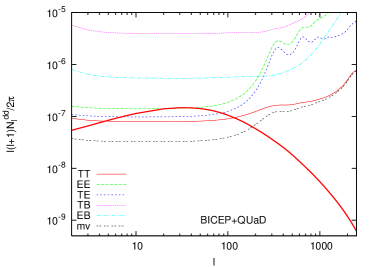
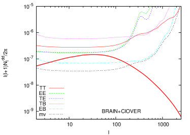
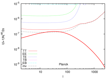
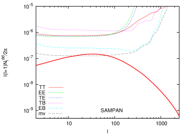
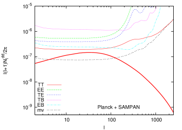
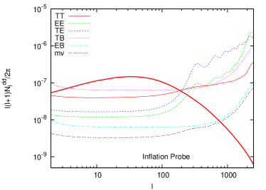
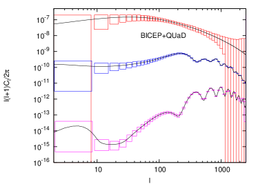
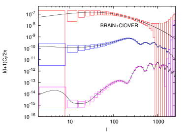
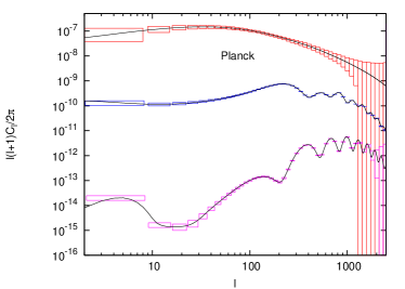
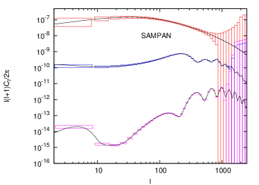
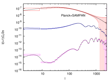
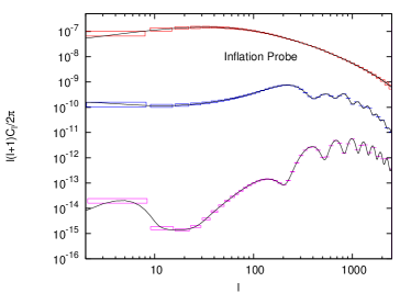
Given this input, the computation of the lensing noise $N_{l}^{dd}$ can be performed numerically following Ref. QE3 . In Fig. 1, we show our results for the lensing noise of each experiment, based on each quadratic estimator and on the combined minimum variance estimator. In Fig. 2 we gather information on the noise for the $TT$, $EE$ and $dd$ power spectra for each experiment. The error-bars $\Delta C_{l}^{aa}$ displayed in Fig. 2 include both cosmic variance and instrumental noise, and assume a multipole binning of width $\Delta l=7$ until $l\sim 70$, and then $\Delta l\sim l/10$

$$\Delta C_{l}^{aa}=\sqrt{\frac{2}{(2l+1)\,\Delta l\,f_{\rm sky}}}(C_{l}^{aa}+N_{l}^{aa})~{}.$$ (19)

The top graphs in Figs. 1 & 2 correspond to the BICEP+QUaD and BRAIN+ClOVER combinations. Computing the Fisher matrix for each pair of experiments is not a trivial task, due to the different sky coverages. We follow a method which is certainly not optimal, but has the merit of simplicity. Since in each case, one experiment is optimized for large scales and the other for smaller scales, we assume that below a given value $l_{c}$ all multipoles are evaluated from BICEP or BRAIN only, while for $l>l_{c}$ they are taken from QUaD or ClOVER. In Eqs. (14, 15), this amounts in considering $f_{\rm sky}$ as a function of $l$, and in replacing $f_{\rm sky}(l)$, $N_{l}^{TT}$ and $N_{l}^{EE}$ by their BICEP/BRAIN value for $l<l_{c}$, or by their QUaD/ClOVER value for $l>l_{c}$. The lensing noise $N_{l}^{dd}$ is then computed for the combined experiment, following the same prescriptions. For each pair of experiments, we optimized the value of $l_{c}$ numerically by minimizing the forecasted error on the total neutrino mass $M_{\nu}$. In both cases, we found that $l\sim 300$ was optimal. This method might be less favorable for BRAIN+ClOVER than for BICEP+QUaD, because the first pair of experiments has a large overlap in $l$-space, for which multipoles could be derived from the two combined datasets.

We find that BICEP+QUaD is able to reconstruct the lensing multipoles $d_{l}^{m}$ in the range $2<l<200$ with an impressively small noise power spectrum $N_{l}^{dd}$. QUaD has both an excellent resolution and a very good sensitivity, and should provide an extremely precise measurement of $T$ and $E$ modes on small angular scales. Therefore, the three quadratic estimators $d(T,T)$, $d(E,E)$ and $d(T,E)$ are particularly efficient.

The main goal of the BRAIN+ClOVER combined experiment is to improve the determination of the $B$-mode performed by BICEP+QUaD, especially on large and intermediate scales ($l<1000$), which are particularly important for detecting gravity waves from inflation. This should be achieved with a sensitivity which is even better than that of BICEP and QUaD, but at the expense of a poorer resolution in the case of ClOVER, leading to large errors for small-scale polarization. In total, this design is roughly equivalent to that of BICEP+QUaD in terms of lensing extraction: BRAIN+ClOVER is also able to reconstruct the lensing multipoles $d_{l}^{m}$ in the range $2<l<200$. The best estimator is now $d(E,B)$, known to be particularly useful, since $E$ and $B$ are correlated only due to lensing. In this sense, future lensing determinations by BRAIN+ClOVER and by BICEP+QUaD can be seen as complementary, and therefore both particularly interesting.

The Planck satellite has a resolution comparable to QUaD, but a poorer sensitivity than the last four experiments. This explains why the lensing noise shown in Fig. 1 looks a bit disappointing: the signal marginally exceeds the noise only around $l\simeq 40$. However, we should keep in mind that Planck will observe the full sky (which leads to $f_{\rm sky}=0.65$, once the galactic cut has been taken into account), while BICEP+QUaD or BRAIN+ClOVER explore only small regions. Therefore, for a given $l$, Planck makes many more independent measurements of multipoles ($T_{l}^{m}$, $E_{l}^{m}$), and consequently, also of $d_{l}^{m}$. In Fig. 2, one can check that Planck still makes a more precise determination of the lensing power spectrum than BICEP+QUaD: both experiments are able to constrain $C_{l}^{dd}$ up to $l\sim 1100$, but the satellite provides smaller errors.

Since Planck is not very sensitive to $B$-modes, and BRAIN is limited by its small sky coverage, there will be room after these two projects for improving $B$-mode observations on large angular scales, in view of observing inflationary gravitational waves. This would be the target of the SAMPAN mini-satellite project, which would be a full-sky experiment with excellent sensitivity but poor resolution. We find that for the minimum variance estimator, the noise $N_{l}^{dd}$ would be at the same level for Planck and SAMPAN. However, it is interesting to note that Sampan has a good $d(E,B)$ estimator, while Planck is better with $d(T,T)$. Therefore, it sounds particularly appealing to combine the two full-sky experiments, that is technically equivalent to assuming a super-experiment with twelve channels (nine from Planck and three from SAMPAN). The results (in the fifth graphs of Figs. 1 & 2) show that with such a combination one could lower the noise $N_{l}^{dd}$ by a factor two for the minimum variance estimator, in order to constrain $C_{l}^{dd}$ up to $l\sim 1300$.

Finally, the (hypothetical) version of the Inflation Probe satellite that we consider here has an extremely ambitious resolution and sensitivity, such that the instrumental error would be better than cosmic variance for the $B$-mode until $l\sim 1500$. For such a precise experiment, assumptions concerning foreground subtraction play a crucial role, since it is very likely that foreground residuals will start dominating the observed power spectrum before instrumental noise. The last graphs in Figs. 1 & 2, which assume perfect foreground cleaning up to $l\sim 2500$, show that lensing multipoles $d_{l}^{m}$ could be recovered up to to $l\sim 800$, while $C_{l}^{dd}$ could be constrained up to at least $l\sim 2500$.

V Future sensitivities to neutrino masses

Free parameters:	8 parameters of minimal $\Lambda$MDM				same + {$\alpha$, $w$, $N_{\rm eff}$}
Lensing extraction:	no	no	yes	yes	no	no	yes	yes
Foreground cleaning:	perfect	none	perfect	none	perfect	none	perfect	none
QUaD+BICEP	1.3	1.6	0.31	0.36	1.5	1.9	0.36	0.40
BRAIN+ClOVER	1.5	1.8	0.34	0.43	1.7	2.0	0.42	0.51
Planck	0.45	0.49	0.13	0.14	0.51	0.56	0.15	0.15
SAMPAN	0.34	0.40	0.10	0.17	0.37	0.44	0.12	0.18
Planck+SAMPAN	0.32	0.36	0.08	0.10	0.34	0.40	0.10	0.12
Inflation Probe	0.14	0.16	0.032	0.036	0.25	0.26	0.035	0.039

Table 2: Expected 1-$\sigma$ error on the total neutrino mass $M_{\nu}$ in eV for various CMB experiments or combinations of them. The first (last) four columns correspond to a $\Lambda$MDM model with eight (eleven) free parameters. For each of the two models, the four columns show the cases with or without lensing extraction, and with two extreme assumptions concerning the foreground treatment: perfect subtraction or no subtraction at all.

For each experiment, we compute the Fisher matrix following Eqs. (14, 15), for a $\Lambda$MDM fiducial model with the parameter values as given below, and considering two possibilities for the number of free parameters that should be marginalized out.

The first possibility is the minimal alternative on the basis of current observations: we marginalize over eight free parameters, standing for the current baryon density $\omega_{\rm b}=\Omega_{\rm b}\,h^{2}$, the current total matter density $\omega_{\rm m}=\Omega_{\rm m}\,h^{2}$, the current dark energy density $\Omega_{\Lambda}$, the total neutrino mass $M_{\nu}$ in eV, the primordial curvature power spectrum amplitude $A_{s}$ and tilt $n_{s}$, the optical depth to reionization $\tau$ and the primordial helium fraction $y_{\rm He}$, to which we assign the values $(\omega_{\rm b},\omega_{\rm m},\Omega_{\Lambda},M_{\nu},\ln[10^{10}A_{s}],n_{s},\tau,y_{\rm He})=(0.023,0.143,0.70,0.1,3.2,0.96,0.11,0.24)$. We assume no spatial curvature and tensor contribution. Note that the reduced Hubble parameter derives from $h=\sqrt{\omega_{\rm m}/(1-\Omega_{\Lambda})}$.

The second possibility, describing non-minimal physical assumptions, is to marginalize over three extra parameters: the scalar tilt running $\alpha$, which can be non-negligible in some inflationary models with extreme assumptions; the dark energy equation-of-state parameter $w$; and finally, extra relativistic degrees of freedom which would enhance the total radiation density, parametrized by the effective number of neutrino species $N_{\rm eff}$ (for instance, $N_{\rm eff}=4$ means that the Universe contains a background of extra relativistic particles with the same density as one extra massless neutrino species). In the fiducial model, these parameters take the values $(\alpha,w,N_{\rm eff})=(0,-1,3)$. Our purpose is to find out whether such extra free parameters open up degeneracy directions in parameter space, that would worsen the sensitivity to neutrino masses. It has been shown in recent analyses that these parameter degeneracies indeed appear with current CMB and LSS data (see Hannestad:2003ye ; Crotty:2004gm for $N_{\rm eff}$ and Hannestad:2005gj ; Ichikawa:2005hi for $w$).

Figure 3: Logarithmic derivatives of the lensing power spectrum $C_{l}^{dd}$ with respect to each cosmological parameter. The derivatives with respect to $\omega_{\rm b}$ and $\omega_{\rm m}$ have been rescaled in order to fit inside the figure.

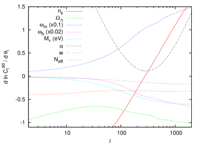
The derivative of the lensing power spectrum $C_{l}^{dd}$ with respect to each of these eleven parameters are shown in Fig. 3, with the exception of the derivatives with respect to $\tau$ and $y_{\rm He}$ which are null, and with respect to $A_{s}$ which is trivial. All derivatives were computed using the public Boltzmann code camb Lewis:1999bs , enabling the highest accuracy options and increasing the accuracy_boost parameter to five. Whenever possible, we evaluated double-sided derivatives, and searched for optimal step sizes such that the results were not affected by numerical errors (from the limited precision of the code) nor by contributions from higher-order derivatives.

We quote the results for the total neutrino mass $M_{\nu}$ in Table 2, assuming either eight or eleven free parameters. For each of the two cases, we compare the forecasted errors with and without lensing extraction, i.e. using either a $2\times 2$ or a $3\times 3$ data covariance matrix, in order to evaluate the impact of the extraction technique. Finally, in each of the four sub-cases, we quote the results obtained assuming perfect foreground cleaning or no cleaning at all, in order to be sure to bracket the true error. Should we trust more the results based on the eight or eleven parameter model? This depends on future results from cosmological observations: in absence of strong observational motivation for extra parameters, one will probably prefer to stick to the simplest paradigm; however, the next years might bring some surprises, like for instance the detection of a variation in the dark energy density.

Let us comment the results for each experiment. The combination QUaD+BICEP benefits a lot from lensing extraction, since the error decreases from approximately $1.5$ eV to at least $0.4$ eV. These results are found to be robust against foreground residuals and extra parameter degeneracies. It is interesting that with QUaD+BICEP it should soon be possible to reach in a near future –using CMB only– the same precision that we have today combining many observations of different types (galaxy-galaxy correlation function, Lyman-$\alpha$ forests) which are affected by various systematics. The situation is almost the same for BRAIN+ClOVER, which should also achieve $\sigma(M_{\nu})\sim 0.4$ eV using lensing extraction.

Planck should make a decisive improvement, lowering the error to $\sigma(M_{\nu})\sim 0.15$ eV, in excellent agreement with the results of Ref. Kaplinghat:2003bh . Note that without lensing extraction the error would be multiplied by three (by four in the case with extra free parameters). We do not find a significant difference between the forecasted errors in the eight and eleven parameter models. SAMPAN alone is slightly more efficient than Planck, and the combination Planck+SAMPAN is the first one to reach $\sigma(M_{\nu})\sim 0.1-0.12$ eV, even in the pessimistic case of large foreground residuals and extra free parameters. Thus these future CMB lensing data could help in breaking the parameter degeneracy between $M_{\nu}$ and $w$ Hannestad:2005gj , that would still be problematic at the level of precision of Planck (without lensing extraction) combined with the galaxy-galaxy correlation function extracted from the Sloan Digital Sky Survey.

Figure 4: 1-$\sigma$ confidence limits on the pairs ($M_{\nu}$, $\theta_{i}$), for each parameter $\theta_{i}$ in our eleven-dimensional model. The red solid (green dashed) contours are those expected for Planck (Inflation Probe). For each case, the smaller (larger) ellipse corresponds to the forecasts with (without) lensing extraction.

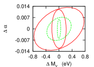
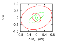
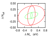
Finally, the version of the Inflation Probe satellite that we consider here is able to reach $\sigma(M_{\nu})=0.035$ eV both in the eight and eleven parameter cases. Note that when we take instead the CMBpol specifications of Ref. Kaplinghat:2003bh , we exactly reproduce their forecast $\sigma(M_{\nu})=0.04$ eV (derived for an intermediate case with ten parameters). It is interesting to see that even with such a precise experiment, the results are robust against foreground contamination, since in absence of any cleaning the forecast error increases only by $15\%$.

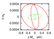
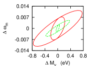
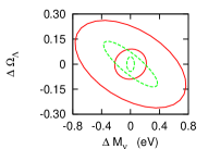
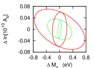
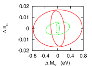
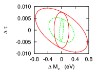
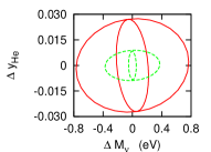
We show in Fig. 4 the correlation between $M_{\nu}$ and each free parameter of the eleven-dimensional model, in the cases of Planck and Inflation Probe, with and without lensing extraction. In the parameter basis used in this work, the neutrino mass appears to be mainly degenerate with $\omega_{m}$, and the lensing extraction process removes most of this degeneracy.

VI Future sensitivities to the neutrino mass splitting

In principle, the LSS power spectrum is not sensitive only to the total mass $M_{\nu}$, but also to the way in which the mass is distributed among the three neutrino states. The reason is twofold: the amount by which the gravitational collapse of matter perturbation is slowed down by neutrinos on small scales depends on the time of the non-relativistic transition for each eigenstate, i.e. on the individual masses; and the characteristic scales at which the free-streaming effect of each neutrino family is imprinted in the power spectrum depends on the value of the wavelengths crossing the Hubble radius at the time of each non-relativistic transition, i.e. again on the individual masses.

The neutrino masses are differently distributed among the three states in the two possible mass schemes, or hierarchies, as shown e.g. in Fig. 1 of Lesgourgues:2004ps . For a total mass $M_{\nu}$ larger than $0.2-0.3$ eV all neutrino states approximately share the same mass $m_{0}=M_{\nu}/3$, in the so-called degenerate region. Instead, for smaller $M_{\nu}$ the splitting between the individual masses is more visible, and for the minimum values of $M_{\nu}$ one finds that in the Normal Hierarchy case (NH) there is only one neutrino state with significant mass, or two degenerate states in the Inverted Hierarchy case (IH). In general, for a given $M_{\nu}$ one can calculate the difference between the matter power spectrum in the two cases, as has been computed numerically in Ref. Lesgourgues:2004ps .

We would like to study whether the lensing power spectrum derived from a very precise CMB experiment like Inflation Probe would be able to discriminate between the two models. For this purpose, we take the eight parameter model of section V and complete it with a ninth parameter: the number of massive neutrinos $N_{\nu}^{\rm massive}$, which could be equal to 1, 2 or 3 (the remaining species are assumed to be exactly massless). In a NH scenario with $M_{\nu}>0.1$ eV, the mass of the third neutrino is not completely negligible: so, we expect the difference between our simplified scenario with $N_{\nu}^{\rm massive}=1$ and that with $N_{\nu}^{\rm massive}=2$ to be more pronounced than the difference between realistic NH and IH scenarios (assuming the same total mass $M_{\nu}$ in all models). This statement is confirmed by the numerical results of Ref. Lesgourgues:2004ps . So, if we could show that an experiment like Inflation Probe will be unable to differentiate between the sketchy $N_{\nu}^{\rm massive}=1$ and $N_{\nu}^{\rm massive}=2$ models, we would conclude that a fortiori it will not discriminate between the NH and IH scenarios.

We repeated the computations of section V with a ninth free parameter $N_{\nu}^{\rm massive}$ with fiducial value $N_{\nu}^{\rm massive}=1$. Note that the parameter $N_{\nu}^{\rm massive}$ should not be confused with the total effective neutrino number $N_{\rm eff}$, which was a free parameter in the last section, and remains fixed to $N_{\rm eff}=3$ in the present one. We found for Inflation Probe – including lensing extraction and assuming perfect foreground cleaning– a one-sigma error $\sigma\left(N_{\nu}^{\rm massive}\right)=2.8$. We conclude that the experiments and techniques discussed in the present paper are far from sufficient for discriminating between the NH and IH scenarios. In any case, as shown in Ref. Lesgourgues:2004ps , future results on the total neutrino mass from very precise cosmological data should be interpreted in a slightly different way for the NH and IH cases.

VII Conclusions

We have studied the ability of future CMB experiments to measure the power spectrum of large scale structure, using some quadratic estimators of the weak lensing deflection field. We inferred the sensitivity of these experiments to the non-zero neutrino masses indicated by neutrino oscillation data. Our aim was to extend the pioneering paper by Kaplinghat, Knox & Song Kaplinghat:2003bh by further investigating several directions.

First, we based our analysis on the following list of forthcoming CMB experiments (either operational, approved or still in project): BICEP, QUaD, BRAIN, ClOVER and Planck, SAMPAN and Inflation Probe, taking into account their detailed characteristics. We found that even before Planck, ground-based experiments should succeed in extracting the lensing map with good precision, and could then significantly improve the bounds on neutrino masses. We also found that the SAMPAN mini-satellite project would be able to reduce the Planck error $\sigma(M_{\nu})$ from approximately $0.15$ eV to $0.10$ eV. Finally, the hypothetical version of Inflation Probe that we considered would reach a spectacular sensitivity of $\sigma(M_{\nu})\sim 0.035$ eV.

We also tried to discuss two questions raised by the analysis of Ref. Kaplinghat:2003bh : first, is it really accurate to base the Fisher matrix computation on perfectly delensed maps on the one hand, and on the reconstructed lensing map on the other? Second, is it realistic to estimate the noise variance of the lensing quadratic estimators without taking into account any residual foreground contamination? Our answer to these two questions is positive: we did not provide an exact treatment of these very technical issues, but we tried to systematically bracket the results between two over-optimistic and over-pessimistic assumptions, and concluded that the error forecast method of Ref. Kaplinghat:2003bh is robust.

Finally, we investigated the issue of parameter degeneracies involving the neutrino mass, by comparing the results in a simpler model than that of Ref. Kaplinghat:2003bh with those in a more complicated one. Our extended cosmological model allows for a scalar tilt running, a dark energy equation of state parameter $w\neq-1$, and extra degrees of freedom parametrized by the effective number of massless neutrinos $N_{\rm eff}$. These extra parameters were not chosen randomly. The tilt running was shown to be slightly degenerate with the neutrino mass in an analysis involving current CMB and LSS data Seljak:2004xh . The same holds for the equation of state of dark energy Hannestad:2005gj and for the effective number of massless neutrinos Hannestad:2003ye ; Crotty:2004gm . However, our results indicate that future CMB experiments will be able to resolve these degeneracies, since we do not find significant discrepancies between the neutrino mass errors obtained for our two cosmological models.

Fortunately, CMB lensing extraction should be regarded as only one of the most promising tools for measuring the absolute neutrino mass with cosmology. It could be combined with future data from tomographic galaxy cosmic shear surveys, which will be very sensitive to neutrino masses Song:2003gg . The cross-correlation of LSS information with CMB temperature anisotropies could also reveal very useful for the purpose of measuring $M_{\nu}$ Ichikawa:2005hi . In the method employed in the present paper, the correlation between temperature and lensing (the $Td$ term) is already taken into account, but it affects the final results only marginally. More interesting should be the cross-correlation of future data from large cosmic shear surveys with that from CMB anisotropies.

In conclusion, our results show that there are good perspectives to detect non-zero neutrino masses using future CMB lensing data, since even in the less favorable case of the smallest $M_{\nu}\simeq 0.05$ eV in the NH mass scheme the Inflation Probe experiment alone could make a marginal detection (between the one and two sigma levels). Obviously the sensitivity is enhanced for larger values of $M_{\nu}$, in particular for the mass degenerate and quasi-degenerate regions but also for the minimum of $M_{\nu}\simeq 0.1$ eV in the IH case. The information on $M_{\nu}$ from analyses of cosmological data will be complementary (and vice versa) to the efforts in terrestrial projects such as tritium beta decay and neutrinoless double beta decay experiments. Of course any positive result on the absolute neutrino mass scale will be a very important input for theoretical models of particle physics beyond the Standard Model.

References

- (1) M. Maltoni, T. Schwetz, M.A. Tórtola and J.W.F. Valle, New J. Phys. 6, 122 (2004) [hep-ph/0405172].
- (2) G.L. Fogli, E. Lisi, A. Marrone and A. Palazzo, Prog. Part. Nucl. Phys., in press [hep-ph/0506083].
- (3) K. Eitel, Nucl. Phys. Proc. Suppl. 143, 197 (2005).
- (4) A. Osipowicz et al. [KATRIN Coll.], hep-ex/0109033.
- (5) H.V. Klapdor-Kleingrothaus et al, Phys. Lett. B 586, 198 (2004) [hep-ph/0404088].
- (6) S.R. Elliott and P. Vogel, Ann. Rev. Nucl. Part. Sci. 52, 115 (2002) [hep-ph/0202264].
- (7) J. Lesgourgues and S. Pastor, in preparation.
- (8) J.R. Bond, G. Efstathiou and J. Silk, Phys. Rev. Lett. 45, 1980 (1980).
- (9) W. Hu, D.J. Eisenstein and M. Tegmark, Phys. Rev. Lett. 80, 5255 (1998) [astro-ph/9712057].
- (10) D.N. Spergel et al [WMAP Coll.], Astrophys. J. Suppl. 148, 175 (2003) [astro-ph/0302209].
- (11) S. Hannestad, JCAP 0305, 004 (2003) [astro-ph/0303076].
- (12) M. Tegmark et al, Phys. Rev. D 69, 103501 (2004) [astro-ph/0310723].
- (13) V. Barger, D. Marfatia and A. Tregre, Phys. Lett. B 595, 55 (2004) [hep-ph/0312065].
- (14) S. Hannestad and G. Raffelt, JCAP 0404, 008 (2004) [hep-ph/0312154].
- (15) P. Crotty, J. Lesgourgues and S. Pastor, Phys. Rev. D 69, 123007 (2004) [hep-ph/0402049].
- (16) R. Rebolo et al, Mon. Not. Roy. Astron. Soc. 353, 747 (2004) [astro-ph/0402466].
- (17) U. Seljak et al, Phys. Rev. D 71, 103515 (2005) [astro-ph/0407372].
- (18) G.L. Fogli et al, Phys. Rev. D 70, 113003 (2004) [hep-ph/0408045].
- (19) K. Ichikawa, M. Fukugita and M. Kawasaki, Phys. Rev. D 71, 043001 (2005) [astro-ph/0409768].
- (20) C.J. MacTavish et al, astro-ph/0507503.
- (21) A.G. Sánchez et al, Mon. Not. Roy. Astron. Soc. 366, 189 (2006) [astro-ph/0507583]
- (22) F. Bernardeau, Astron. Astrophys. 324, 15 (1997) [astro-ph/9611012].
- (23) M. Zaldarriaga and U. Seljak, Phys. Rev. D 58, 023003 (1998) [astro-ph/9803150].
- (24) U. Seljak and M. Zaldarriaga, Phys. Rev. Lett. 82, 2636 (1999) [astro-ph/9810092].
- (25) D.J. Eisenstein, W. Hu and M. Tegmark, Astrophys. J. 518, 2 (1998) [astro-ph/9807130].
- (26) J. Lesgourgues, S. Pastor and S. Prunet, Phys. Rev. D 62, 023001 (2000) [hep-ph/9912363].
- (27) S. Hannestad, Phys. Rev. D 67, 085017 (2003) [astro-ph/0211106].
- (28) J. Lesgourgues, S. Pastor and L. Perotto, Phys. Rev. D 70, 045016 (2004) [hep-ph/0403296].
- (29) A.R. Cooray, Astron. Astrophys. 348, 31 (1999) [astro-ph/9904246].
- (30) M. Kaplinghat, L. Knox and Y.S. Song, Phys. Rev. Lett. 91, 241301 (2003) [astro-ph/0303344].
- (31) Y.S. Song and L. Knox, Phys. Rev. D 70, 063510 (2004) [astro-ph/0312175].
- (32) C.M. Hirata and U. Seljak, Phys. Rev. D 68, 083002 (2003) [astro-ph/0306354].
- (33) N. Bartolo, E. Komatsu, S. Matarrese and A. Riotto, Phys. Rep. 402, 103 (2004) [astro-ph/0406398].
- (34) U. Seljak, Astrophys. J. 463, 1 (1996) [astro-ph/9505109].
- (35) T. Okamoto and W. Hu, Phys. Rev. D 67, 083002 (2003) [astro-ph/0301031].
- (36) W. Hu, Astrophys. J. 557, L79 (2001) [astro-ph/0105424].
- (37) W. Hu and T. Okamoto, Astrophys. J. 574, 566 (2002) [astro-ph/0111606].
- (38) A. Cooray and M. Kesden, New Astron. 8, 231 (2003) [astro-ph/0204068].
- (39) M. Tegmark, A. Taylor and A. Heavens, Astrophys. J. 480, 22 (1997) [astro-ph/9603021].
- (40) A. Lewis, A. Challinor and A. Lasenby, Astrophys. J. 538, 473 (2000) [astro-ph/9911177].
- (41) A. Amblard, C. Vale and M.J. White, New Astron. 9, 687 (2004) [astro-ph/0403075].
- (42) A. Cooray, M. Kamionkowski and R.R. Caldwell, Phys. Rev. D 71, 123527 (2005) [astro-ph/0503002].
- (43) M. Tegmark, D.J. Eisenstein, W. Hu and A. de Oliveira-Costa, Astrophys. J. 530, 133 (2000) [astro-ph/9905257].
- (44) N. Ponthieu et al, Astron. Astrophys. 444, 327 (2005) [astro-ph/0501427].
- (45) B.G. Keating et al, in Polarimetry in Astronomy, ed. by S. Fineschi, Proceedings of the SPIE 4843, 284 (2003).
- (46) S. Church et al [QUaD Coll.], New Astron. Rev. 47, 1083 (2003).
- (47) M. Piat et al [BRAIN-CLOVER Coll.], SF2A 2004 proceedings (2004) [astro-ph/0412590].
- (48) B. Maffei et al. [BRAIN-ClOVER Coll.], EAS Publications Series 14, 251 (2005).
- (49) J.A. Tauber, Adv. Space Res. 34, 491 (2004).
- (50) F.R. Bouchet et al, SF2A 2005 proceedings (2005) [astro-ph/0510423].
- (51) J. Bock, private communication.
- (52) M. Bowden et al, Mon. Not. Roy. Astron. Soc. 349, 321 (2004) [astro-ph/0309610].
- (53) The Planck Consortia, “The Scientific Programme of Planck 2004 (Blue Book)”, ESA Publication Division (2005).
- (54) S. Hannestad, Phys. Rev. Lett. 95, 221301 (2005) [astro-ph/0505551].
- (55) K. Ichikawa and T. Takahashi, astro-ph/0510849.