Reconciliation of Statistical Mechanics
and Astro-Physical Statistics.
The errors of conventional canonical Thermostatistics

Abstract

Conventional thermo-statistics address infinite homogeneous systems within the canonical ensemble. (Only in this case this is equivalent to the fundamental microcanonical ensemble.) However, some 170 years ago the original motivation of thermodynamics was the description of steam engines, i.e. boiling water. Its essential physics is the separation of the gas phase from the liquid. Of course, boiling water is inhomogeneous and as such cannot be treated by conventional thermo-statistics. Then it is not astonishing, that a phase transition of first order is signaled canonically by a Yang-Lee singularity. Thus it is only treated correctly by microcanonical Boltzmann-Planck statistics. It turns out that the Boltzmann-Planck statistics is much richer and gives fundamental insight into statistical mechanics and especially into entropy. This can be done to a far extend rigorously and analytically. As no extensivity, no thermodynamic limit, no concavity, no homogeneity is needed, it also applies to astro-physical systems. The deep and essential difference between “extensive” and “intensive” control parameters, i.e. microcanonical and canonical statistics, is exemplified by rotating, self-gravitating systems. In the present paper the necessary appearance of a convex entropy $S(E)$ and negative heat capacity at phase separation in small as well macroscopic systems independently of the range of the force is pointed out. Thus the old puzzle of stellar statistics is finally solved, the appearance of negative heat capacity which is forbidden and cannot appear in the canonical formalism.

Presented at the NBS2005 at the Observatoire de Paris

1 Introduction

Conventional statistical mechanics addresses homogeneous macroscopic systems in the thermodynamic limit. These are traditionally treated in canonical ensembles controlled by intensive temperature $T$, chemical potential $\mu$ and/or pressure $P$. In the canonical ensemble the heat capacity is given by the fluctuation of the energy $<\!\!(\delta E)^{2}\!\!>/T^{2}\geq 0$.

As in astro-physics the heat capacity is often negative it is immediately clear that astro-physical systems are not in the canonical ensemble. This was often considered as a paradoxical feature of the statistics of self-gravitating systems. Here we will show that this is not a mistake of equilibrium statistics when applied to self-gravitating systems but is a generic feature of statistical mechanics of any many-body systems at phase separation, independently of the range of the interactions, ref.gross219 .

As the original motivation of thermodynamics was the understanding of boiling water in steam-engines, this points to a basic misconception of conventional canonical thermo-statistics. As additional benefit of our reformulation of the basics of statistical mechanics by microcanonical statistics there is a rather simple interpretation of entropy, the characteristic entity of thermodynamics.

2 What is entropy?

Boltzmann, ref.boltzmann1877 , defined the entropy of an isolated system in terms of the sum of all possible configurations, $W$, which the system can assume consistent with its constraints of given energy, volume, and further conserved constraints:

S=k*lnW (1)

as written on Boltzmann’s tomb-stone, with

$$W(E,N,V)=\int{\frac{d^{3N}\stackrel{{\scriptstyle\rightarrow}}{{p}}\;d^{3N}\stackrel{{\scriptstyle\rightarrow}}{{q}}}{N!(2\pi\hbar)^{3N}}\epsilon_{0}\;\delta(E-H\{\stackrel{{\scriptstyle\rightarrow}}{{q}},\stackrel{{\scriptstyle\rightarrow}}{{p}}\})}$$ (2)

in semi-classical approximation. $E$ is the total energy, $N$ is the number of particles and $V$ the volume. Or, more appropriate for a finite quantum-mechanical system:

$$W(E,N,V)=Tr[\mathcal{P}_{E}]=\sum{\scriptscriptstyle\begin{array}[]{ll}\mbox{all eigenstates n of H with given N,$V$,}\\ \mbox{and }E<E_{n}\leq E+\epsilon_{0}\end{array}}$$

and $\epsilon_{0}\approx$ the macroscopic energy resolution. This is still up to day the deepest, most fundamental, and most simple definition of entropy. There is no need of the thermodynamic limit, no need of concavity, extensivity, and homogeneity. Schrödinger was wrong saying that microcanonical statistics is only good for diluted systems, ref.schroedinger46 . It may very well also address the solid-liquid transition ref.gross213 and even self-gravitating systems as we will demonstrate in this article. In its semi-classical approximation, eq.(2), $W(E,N,V,\cdots)$ simply measures the area of the sub-manifold of points in the $6N$-dimensional phase-space ($\Gamma$-space) with prescribed energy $E$, particle number $N$, volume $V$, and some other time invariant constraints which are here suppressed for simplicity. Because it was Planck who coined it in this mathematical form, I will call it the Boltzmann-Planck principle.

The Boltzmann-Planck formula has a simple but deep physical interpretation: $W$ or $S$ measure our ignorance about the complete set of initial values for all $6N$ microscopic degrees of freedom which are needed to specify the $N$-body system unambiguously, ref.kilpatrick67 . To have complete knowledge of the system we would need to know [within its semiclassical approximation (2)] the initial positions and velocities of all $N$ particles in the system, which means we would need to know a total of $6N$ values. Then $W$ would be equal to one and the entropy, $S$, would be zero. However, we usually only know the value of a few parameters that are conserved or change slowly with time, such as the energy, number of particles, volume and so on. We generally know very little about the positions and velocities of the particles. The manifold of all these points in the $6N$-dim. phase space, consistent with the given conserved macroscopic constraints of $E,N,V,\cdots$, is the microcanonical ensemble, which has a well-defined geometrical size $W$ and, by equation (1), a non-vanishing entropy, $S(E,N,V,\cdots)$. The dependence of $S(E,N,V,\cdots)$ on its arguments determines completely thermostatics and equilibrium thermodynamics.

Clearly, Hamiltonian (Liouvillean) dynamics of the system cannot create the missing information about the initial values - i.e. the entropy $S(E,N,V,\cdots)$ cannot decrease. As has been further worked out in ref.gross183 and more recently in ref.gross207 the inherent finite resolution of the macroscopic description implies an increase of $W$ or $S$ with time when an external constraint is relaxed, c.f.chapter 5. Such is a statement of the second law of thermodynamics, ref.prigogine71 , which requires that the internal production of entropy be positive or zero for every spontaneous process. Analysis of the consequences of the second law by the microcanonical ensemble is appropriate because, in an isolated system (which is the one relevant for the microcanonical ensemble), the changes in total entropy must represent the internal production of entropy, see above, and there are no additional uncontrolled fluctuating energy exchanges with the environment.

3 No phase separation (no boiling water) without convex non-extensive $S(E)$.

The weight $e^{S(E)-E/T}$ of configurations with energy E in the definition of the canonical partition sum

$$Z(T)=\int_{0}^{\infty}{e^{S(E)-E/T}dE}$$ (3)

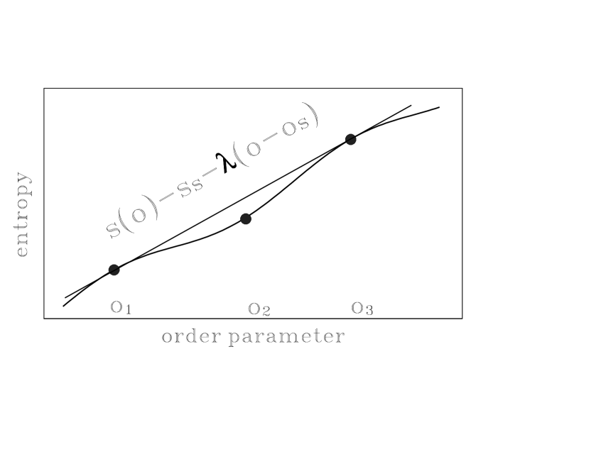
becomes here bimodal, at the transition temperature it has two peaks, the liquid and the gas configurations which are separated in energy by the latent heat. Consequently $S(E)$ must be convex (like $y=x^{2}$) and the weight in (3) has a minimum between the two pure phases. Of course, the minimum can only be seen in the microcanonical ensemble where the energy is controlled and its fluctuations forbidden. Otherwise, the system would fluctuate between the two pure phases (inter-phase fluctuation) by an, for macroscopic systems even macroscopic, energy $\Delta E\sim E_{lat}\propto N$ of the order of the latent heat. I.e. the convexity of $S(E)$ is the generic signal of a phase transition of first order and of phase-separation, ref.gross174 . This applies also to macroscopic systems coupled by short or long-range interactions. Of course, even there phase-separation exists and there is a minimum (convexity) in $S(E)$ and, consequently, negative heat capacitygross219 .

Figure 1: Convex intruder in the entropy as function of an conserved order parameter. Gibbs double tangent rule $\equiv$ concave hull. The derivative gives the Maxwell line in $T(E)$. Three values of the order parameter correspond to the single intensive “temperature” (inverse slope $T=1/\lambda$). At $o_{1}$ the system is in the “liquid” phase, at $o_{3}$ in its “gas” phase. The difference $o_{3}-o_{1}$ is the latent “heat” and of macroscopic size $\propto N$.

It must be emphasized: In conventional canonical statistics phase-separated systems are treated by artificial constructions of two coexisting simple configurations of each phase like a single drop with vapor around (Wulff-construction). But this is not a common ensemble of various droplets with its inter-phase fluctuations leading e.g. to a negative heat capacity. Such macroscopic energy fluctuations and the resulting negative heat capacity are already early discussed in high-energy physics by Carlitz, ref.carlitz72 .

4 Application to astrophysics

Classical Boltzmann-Planck microcanonical statistics applies very well to the equilibrium of self-gravitating systems provided we put the system into a box (ignoring slow evaporation) and use a hard core in the interaction at short distances where anyhow non-gravitational physics like hydrogen burning dominates gravity. Padmanabhan in his stimulating review ref.padmanabhan02 discussed this point in detail.

We simplify the original many-body problem by the mean-field approximation, details in refgross207 . Here the (certainly also important) many-body correlations are ignored. The entropy is then a function of the one-body densities $\rho(\mbox{\boldmath r})$. $S(E,\rho)$ is maximized and a closed equation for the optimal one-body density distributions obtained. To get this result and to get finite $\rho(\mbox{\boldmath r})$ the short-distance cut-off and a hard core in the two-body interaction $U(\mbox{\boldmath r-r'})$ is essential. The resulting mean-field theory therefore does not lead to an isothermal sphere. The latter is a solution of Poisson’s equation (ref.padmanabhan02 ) with a strict $1/r$ interaction.

Moreover, for equilibrium one does not need any exotic q-deformed statistics, ref.gross203 ; tsallis04 . The error of ref.tsallis04 is the use of a generalized variant of Boltzmann-Gibbs canonical ensemble instead of the basic microcanonical one, a point on which Tsallis seems to agree in his discussion in ref.tsallis04 , see also ref.gross207 .

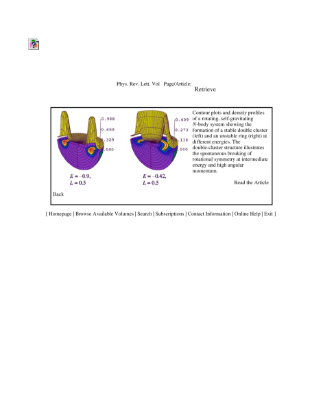
In fig. 2 we show the equilibrium distributions of self-gravitating systems under large angular-momentum in the mean-field approximation:

Figure 2: Rotating multi-star-systems at equilibrium. The left shows a rotating double-star system in the DC phase, c.f. fig.3. This is an inhomogeneous phase, analog to nuclear multifragmentation. The right is one of the many different, unstable, configurations existing in the mixed phase with negative heat capacity. Here the system fluctuates between such ring systems, systems of stars rotating around a central star but also mono-stars and eventual gas. This region is very interesting but must still be more investigated. [Cover page of Phys.Rev.Lett. vol 89, (July 2002)]

The necessity of using “extensive” instead of “intensive” control parameters is explicit in astrophysical problems. E.g.: for the description of rotating stars one conventionally works at a given temperature and fixed angular velocity $\Omega$ c.f. ref.chavanis03 . Of course in reality there is neither a heat bath nor a rotating disk. Moreover, the latter scenario is fundamentally wrong as at the periphery of the disk the rotational velocity may even become larger than velocity of light. Non-extensive systems like astro-physical ones do not allow a “field-theoretical” description controlled by intensive fields !

Figure 3: Phase diagram of rotating self-gravitating systems in the energy-angular-momentum $(E,L)$-plane. DC: region of double-stars, G: gas phase, SC: single stars. In the mixed region one finds various exotic configurations like ring-systems in coexistence with gas, double stars or single stars. In this region of phase-separation the heat capacity is negative and the entropy is convex. The dashed lines $E-L=-1$ (left) and $E=L$ (right) delimit the region where systematic calculations were carried out. At a few points outside of this strip some calculations like the left of fig.(2) were also done.

E.g. configurations with a maximum of random energy on a rotating disk, i.e. at fixed rotational velocity $\Omega$ (which is intensive):

$$E_{random}=E-\frac{\Theta\Omega^{2}}{2}-E_{pot}$$ (4)

and consequently with the largest entropy are the ones with smallest moment of inertia $\Theta$, compact single stars. Just the opposite happens when the angular-momentum $L$ (extensive) and not the angular velocity $\Omega$ is fixed:

$$E_{random}=E-\frac{L^{2}}{2\Theta}-E_{pot}.$$ (5)

Then configurations with large moment of inertia are maximizing the phase space and the entropy. I.e. eventually double or multi stars are produced, as observed in reality.

In figure 3 one clearly sees the rich and realistic microcanonical phase-diagram of a rotating gravitating system controlled by the conserved “extensive” parameters energy and angular-momentum, ref.gross187 .

5 On the Second Law

Also the Second Law becomes significantly more transparent within microcanonical statistics:

Many formulations of the second law exist. The understanding of entropy is sometimes obscured by frequent use of the Boltzmann-Gibbs canonical ensemble, and thermodynamic limit; and the relationship of entropy to the second law is often beset with confusion between external transfers of entropy and its internal production. Perhaps the clearest statement is by Prigogine, ref.prigogine71 : He distinguishes between internal and external entropy transfer. Whereas the transfer $d_{ext}S=dQ/T$ to an external heat bath can be positive, negative, or zero, the internal generation of entropy $d_{int}S$ within the system is necessarily $d_{int}S\geq 0$. This is the sharpest formulation of the second law. $d_{int}S$ is best seen in the microcanonical ensemble, as there are no couplings to any heat bath and no sometimes uncontrolled exchanges of energy with it.

The second law is then most rigorously given by equation (6):

$$dS = d_{ext}S+d_{int}S$$

$$d_{ext}S =$$ positive, negative, or zero

$$d_{int}S \geq 0$$ (6)

A geometric visualization how an equilibrium distribution in the $6N$-dim phase space expands into a (fat)-fractal (Gibbs ink lines) after a constraint, here the wall between the phase-space volumes between $V_{1}$ and $V_{2}$ is suddenly released is given by figure (4).

$V_{a}$                 $V_{b}$

$t<t_{0}$

$\longrightarrow$ $V_{a}+V_{b}$ $t>t_{0}$

Figure 4: The sudden expansion in phase-space of an equilibrized system left into a larger phase-space at $t>t_{0}$ right. When at $t_{0}$ the wall closing volume $V_{a}$ is suddenly removed, the compact set $M(t<t_{0})$, left side, develops into an increasingly folded “spaghetti”-like, though still compact, distribution in phase-space with rising time $t>t_{0}$, the Gibbs’ ”ink-lines”. The right figure shows only the early form of the distribution. At much larger times it will become more and more fractal and finally dense in the new phase space. The grid illustrates the boxes of the box-counting method. All boxes with size $\delta^{6N}$ which overlap with $M(t)$ are counted by $N_{\delta}$ in eq.(7)

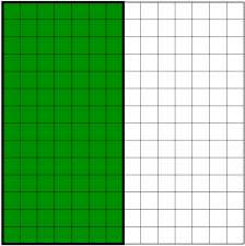
The Liouville theorem tells us that the (Riemannian-) size of it as given by eq.(2) does not change. Keeping in mind that due to the redundant information about the system (c.f. chapter 2) it is in general impossible to distinguish a point inside the fractal from a neighboring point outside. Therefore the proper way to “measure” the size of the manifold is by its box-counting “measure”. I.e. the phase-space integrals in eq.(2) or eq.(2) have to be calculated by the box-counting volume $\mbox{vol}_{box}{\bf M}$ as is explained in fig.(4) (details in refs.gross183 ; gross207 ):

$$\mbox{vol}_{box}[{\bf M}(E,N,t\gg t_{0})]:=\underline{\lim}_{\delta\to 0}\delta^{6N}N_{\delta}[{\bf{M}}(E,N,t\gg t_{0})]$$ (7)

which is $\geq\mbox{vol}_{box}[{\bf M}(E,N,t<t_{0})]$. That is the Second Law.

6 Further challenges

The story of applying microcanonical statistics to self-gravitating systems and eventually to cosmology is far open. There are many questions to answer, e.g.:

There is the problem of statistics in an expanding universe as discussed by Padmanabhan ref.padmanabhan02 , the question of defining Boltzmann-Planck statistics in general relativity and connected the problem of avoiding field-theoretical descriptions with intensive statistical control-parameters or using them despite the fact that first order transitions demand extensive control parameters as discussed here. The present author, coming from far away from nuclear and statistical physics, is open for any helpful suggestion. An interdisciplinary meeting like this NBS2005 is here very important. I like to thank Francoise Combes and Raoul Robert for this great opportunity.

7 Conclusion

Conventional canonical statistics is insufficient to handle the original goal of Thermodynamics, phase separations with their characteristic inter-phase fluctuations. Here the microcanonical ensemble is much richer and leads to negative specific heat. This is thus not a characteristics of self-gravitating systems. Phase transitions can be found without the thermodynamic limit, without homogeneity, concavity, and extensivity. Microcanonical statistics opens to a much wider class of applications as e.g. astrophysical systems. Moreover it gives a simple formulation and proof of the second law.

References

- (1) D.H.E. Gross. Negative heat-capacity at phase-separations in microcanonical thermostatistics of macroscopic systems with either short or long-range interactions. http://arXiv.org/abs/cond–mat/0509234, (2005).
- (2) L. Boltzmann. Über die Beziehung eines algemeinen mechanischen Satzes zum Hauptsatz der Wärmelehre. Sitzungsbericht der Akadamie der Wissenschaften, Wien, II:67–73, 1877.
- (3) E. Schrödinger. Statistical Thermodynamics, a Course of Seminar Lectures, delivered in January-March 1944 at the School of Theoretical Physics. Cambridge University Press, London, 1946.
- (4) D.H.E. Gross and J.F. Kenney. The microcanonical thermodynamics of finite systems: The microscopic origin of condensation and phase separations; and the conditions for heat flow from lower to higher temperatures. Journal of Chemical Physics, 122:224111; http://arXiv.org/abs/cond–mat/0503604, (2005).
- (5) J.E. Kilpatrick. Classical thermostatistics. In H. Eyring, editor, Statistical Mechanics, number II, chapter 1, pages 1–52. Academic Press, New York, 1967.
- (6) D.H.E. Gross. Ensemble probabilistic equilibrium and non-equilibrium thermodynamics without the thermodynamic limit. In Andrei Khrennikov, editor, Foundations of Probability and Physics, number XIII in PQ-QP: Quantum Probability, White Noise Analysis, pages 131–146, Boston, October 2001. ACM, World Scientific.
- (7) D.H.E. Gross. A new thermodynamics from nuclei to stars. Entropy, 6:158–179,http://arXiv.org/abs/cond–mat/0505450, (2004).
- (8) P. Glansdorff and I. Prigogine. Thermodynamic Theory of Structure, Stability and Fluctuations. John Wiley& Sons, London, 1971.
- (9) D.H.E. Gross. Microcanonical thermodynamics: Phase transitions in “Small” systems, volume 66 of Lecture Notes in Physics. World Scientific, Singapore, 2001.
- (10) R.D. Carlitz. Hadronic matter at high density. Phys.Rev.D, 5:3231–3242, 1972.
- (11) T. Padmanabhan. Statistical mechanics of gravitating systems in static and cosmological backgrounds. http://arXiv:astro–ph/020613, 2002.
- (12) E.V. Votyakov, A. De Martino, and D.H.E. Gross. Thermodynamics of rotating self-gravitating systems. Eur. Phys. J B, 29:593; http://arXiv.org/abs/cond–mat/0207153, 2002).
- (13) D.H.E. Gross. Classical equilibrium thermostatistics, ”Sancta Sanctorum of Statistical Mechanics”, from Nuclei to Stars. Physica A, 340/1-3:76–84, http://arXiv.org/abs/cond–mat/0311418, (2004).
- (14) C. Tsallis. What should a statistical mechanics satisfy to reflect nature? pages http://arXiv.org/abs/cond–mat/0403012, 2004.
- (15) P.H. Chavanis and M. Rieutord. Statistical mechanics and phase diagrams of rotating self-gravitating fermions. Astron. Astrophys., 412:1, http://arXiv:astro–ph/0302594, 2003.
- (16) E.V. Votyakov, H.I. Hidmi, A. De Martino, and D.H.E. Gross. Microcanonical mean-field thermodynamics of self-gravitating and rotating systems. Phys.Rev.Lett., 89:031101–1–4; http://arXiv.org/abs/cond–mat/0202140, (2002).