Radiative zone solar magnetic fields and g-modes
Abstract
We consider a generalized model of seismic-wave propagation that takes into account the effect of a central magnetic field in the Sun. We determine the g-mode spectrum in the perturbative magnetic field limit using a one-dimensional Magneto-Hydrodynamics (MHD) picture. We show that central magnetic fields of about 600-800 kG can displace the pure g-mode frequencies by about 1%, as hinted by the helioseismic interpretation of GOLF observations.
keywords:
MHD – Sun: helioseismology – Sun: interior – Sun: magnetic fields.1 Introduction
Currently there is very little direct information about the structure and strength of magnetic fields in the radiative zone (RZ) of the Sun, for a short review see Introduction of the paper (Burgess et al., 2004a). Some authors argue that for the young Sun ( Myr) relatively small fields, kG (Moss, 2003) and Gauss (Kitchatinov, Jardine & Collier-Cameron, 2001) could survive, being relic fields captured from the primordial ones in the protostar plasma. For the Sun at the present epoch there is an upper bound of MG near the tachocline obtained from the magnetic splitting of acoustic oscillations (Ruzmaikin & Lindsey, 2002). However, some authors have considered very strong magnetic fields in the RZ, up to 30 MG (Couvidat, Turck-Chièze & Kosovichev, 2003).
Here we suggest a new way to estimate the magnetic field strengths in the RZ of the Sun by relating them to the frequency shifts of g-mode candidates suggested by the first observations made with the GOLF (Global Oscillations at Low Frequencies) experiment (Turck-Chièze et al., 2004). We discuss some effects of RZ magnetic fields which could explain the displacement of g-mode frequencies with respect to the theoretical frequencies calculated in the absence of magnetic field. Indeed the existence of such shifts are hinted in GOLF’s data. If eventually confirmed by further data, the idea that RZ magnetic fields cause such frequency shifts would provide us with a useful tool to estimate their magnitude.
In order to find spectra of seismic waves accounting for the magnetic field in the RZ a number of assumptions is required. For example:
-
1.
We consider ideal MHD neglecting both the heat conductivity and viscosity contributions to energy losses, as well as the ohmic dissipation.
-
2.
We linearize the MHD equations about a static background configuration, i.e. a background configuration which is time independent and for which the background fluid velocity vanishes, .
-
3.
We assume the fluctuations to be adiabatic, with the contributions of fluctuations to the heat source vanishing: .
-
4.
Moreover, we consider a fully ionized ideal gas, so that the thermodynamic quantity, first adiabatic exponent , is time independent and uniform. For numerical estimates we will take for hydrogen plasma.
-
5.
We adopt the Cowling approximation, which amounts to the neglect of perturbations of the gravitational potential, (i.e.: ).
-
6.
We assume a rectangular geometry with Cartesian coordinates: , , and , where corresponds to the solar radial direction. The background quantities vary along the direction only (which implies the local gravitational acceleration, , is directed along the axis, but in opposite direction). We also take a constant, uniform background magnetic field, , pointing along the axis.
-
7.
The background mass-density profile is assumed to be exponential, , for constant and . The conditions of hydrostatic equilibrium for the background then determine the profiles of thermodynamic quantities, and in particular imply is a constant. We assume that the Brunt-Väisälä frequency is zero in the convective zone (CZ) and non-zero, but constant in the RZ.
In what follows, we shall again specify the assumptions used, as they are needed, in order to keep clear which results rely on which assumptions.
Note that, deep within the radiative zone, the last approximation above holds to very good approximation for real mass-density profiles obtained by Standard Solar Models, provided we identify the direction with the radial direction. The constancy of in this region is also expected since the highly-ionized plasma satisfies an ideal gas equation-of-state to good approximation. The rectangular geometry provides a reasonable approximation so long as we do not examine too close to the solar centre. What is important about our choice for is that it is slowly varying in the region of interest, and it is perpendicular to both and all background gradients, , , etc.
As suggested in (Burgess et al., 2004a) such one-Dimensional (1-D) picture can be fully described in analytical terms in contrast to the 3-D case. There are two parameters which describe the spectra of magneto-gravity waves (Burgess et al., 2004a): (i) strength of the background magnetic field and (ii) the dimensionless transversal wave number . Here is the density scale height and is the projection of the wavevector onto the x axis. Let us estimate the value of the transversal wave number that could be relevant for the g-mode candidates observed on the photosphere.
Since g-modes decay in the CZ as , only modes with low transversal wave number (long wave lengths) could be seen at the photosphere. This follows from the simple estimate for the longitudinal fluid velocity which is directed along the Sun-Earth line and causes the Doppler shifts of optic lines registered by the GOLF experiment:
| (1) |
This formula comes from Eq. (14) (equivalent to our Eq. (10)) and Eq. (30) of Ref. (Burgess et al., 2004a) for the decaying solution , where is the -component of the magnetic field perturbation.
Here in the right hand side we substituted the sensitivity of the GOLF-instrument to the minimum fluid speed, , while in the left hand side we substituted the frequency estimate and the wave length through the CZ: . For instance, substituting for the magnetic field perturbation, , for the Brunt-Väisälä frequency in the RZ, (Bahcall, 1988) for the density scale height, one obtains , from which the estimate comes.
We organize our presentation as follows. In Section 2 we formulate the MHD model for an ideal plasma. In Section 3 we linearize the full set of MHD equations and then derive a single master equation for the z-component of the perturbation velocity . This component leads to the Doppler shift of the optic frequencies measured in helioseismic experiments. In Subsection 3.1 we check the validity of the master equation against the well-known case of standard helioseismology in an isotropic plasma, without magnetic fields. In Subsection 3.2 we derive the simplified master equation in the perturbative limit. In this limit there are no MHD (slow or Alfvén) resonances within the Sun, a situation which was treated in (Burgess et al., 2004a). This perturbative method allows us to use a standard quantum mechanical 1-D approach to determine an exact analytical spectrum of g-modes in the presence of RZ magnetic fields. In Section 4 we summarize our results.
2 Basic ideal MHD equations
We describe the Sun as an ideal hydrodynamical system characterized by nonlinear MHD equations. The mass conservation law for the total density can be written as
| (2) |
The total pressure is a sum of equilibrium, , and non-equilibrium, , parts, . Since viscosity can be neglected, momentum is conserved according to
| (3) |
Here the total pressure consists of two terms: the equilibrium and non-equilibrium parts. The first is expressed as and obeys the equation . The non-equilibrium part of the total pressure involves non-linear terms coming from the total magnetic field .
The evolution of the magnetic field is governed by Faraday’s equation,
| (4) |
where is the compressibility of the gas. Finally the conservation of entropy leads to the energy conservation law for an ideal plasma,
| (5) |
where is the total gas pressure.
3 Linear MHD master equation
For definiteness here we consider the same generalized helioseismic model already proposed in Ref. (Burgess et al., 2004a), adopting an approximately rectangular rather than cylindrical, geometry. In this case it is convenient to choose a Cartesian coordinate system whose z-axis is the “radial”direction; opposite to the local acceleration, . With this choice we take in the range , where represents the solar center and denotes the solar surface. The radiative zone corresponds to .
The model assumes the background magnetic field to be directed along the x-axis , ensuring that physical gradients lie along the z-axis. Such a field mimics both a toroidal field lying in the equatorial plane and a poloidal field perpendicular to the equatorial plane.
We now linearize the above MHD equations (2-5), so that all variables are split into background and fluctuating Euler quantities, , with denoting small fluctuations about the background value . In what follows we also neglect rotation of the Sun, so that the background velocity is zero, . Moreover, we assume that the MHD perturbations are independent of , which implies that , leaving just six perturbation functions, instead of eight.
In addition, following (Ruderman, Hollweg & Goossens, 1997), we consider plane waves propagating along the -axis and therefore the dependence of all functions on the coordinates can be reduced to just , with being the phase velocity. This can be done since all functions depend only on the harmonic factor .
This way all perturbations are functions of two variables, , and the linearized MHD equations involve partial derivatives over and . Notice that and .
Let us rewrite the initial system for the six functions in Eqs. (2-5) expressing all of them through just two quantities, and . One obtains:
| (6) |
| (7) |
| (8) |
| (9) |
| (10) |
| (11) |
We introduced above the important coefficients which in turn are functions of “z” via , the Alfvén velocity , and the sound velocity :
| (12) |
where is the squared cusp velocity. The zeros of the last coefficient correspond to the slow () or Alfvén (, ) resonances respectively.
Differentiating Eq. (6) over and using the next two equations one gets the master equation for the function as:
| (13) |
It is easy to see that, neglecting gravity, our generalized equations (6)-(3) recover the total system (34)-(38) derived in (Ruderman, Hollweg & Goossens, 1997) and Eq. (3) coincides with Eq. (39) in (Ruderman, Hollweg & Goossens, 1997). In case of the constant gravity, =const, while the sound velocity depends on the varying height scale , Eq. (3) recovers Eq. (7) in (Miles, Allen & Roberts, 1992).
For simplicity we consider below the particular case of uniform and constant magnetic field, =const, constant gravity, =const, and density scale height, =const. Therefore the sound speed and the Brunt-Väisälä frequency are also constants in RZ, =const, =const. This is somewhat of a simplification of the real Sun, but it allows us to derive qualitative estimates of the magnetic field corrections to the pure g-mode spectrum.
In what follows in our numerical estimates we will use the following values: (hydrogen plasma), , (Bahcall, 1988), hence , .
Separating in master equation (3) the exponential dependence and taking into account the background density profile , one gets the ordinary second order equation111Here we have corrected the factor in front of the first derivative in Eq. (16) of (Burgess et al., 2004a) changing . This does not affect the MHD spectra found there.:
| (14) |
This equation generalizes Eq. (16) of our work (Burgess et al., 2004a) accounting for the compressibility parameter ( for hydrogen plasma with ). Note that is small for very low frequencies of g-modes , , and therefore it was neglected in the problem considered in (Burgess et al., 2004a).
3.1 Zero magnetic field limit
For with the use of the transformation Eq. (3) converts into
| (15) |
This 1-D MHD equation coincides with the 3-D oscillation Eq. (7.90) in (Christensen-Dalsgaard, 2003):
| (16) |
here we have substituted the acoustical cut-off frequency and put , see Eq. (4.60) in (Christensen-Dalsgaard, 2003).
We would like to stress that, in the JWKB approximation for low frequency g-modes, , , both equations (15) and (16) lead to the analogous spectra:
| (17) |
where is the radial order of the wave, and the transversal wave number is the 1-D analogue of the angular degree in the 3-D case.
Let us denote the factor in brackets in Eq. (15) as ,
| (18) |
here is the dimensionless wave number, . Eq. (15) can be rewritten using Eq. (18) as
| (19) |
In RZ where one obtains the solution of Eq. (19) in the form , where is a constant. It accounts for the boundary condition at the center of the Sun. In CZ we approximate Brunt-Väisälä frequency by the value . In that case tends to . Taking into account a second boundary condition, that there are no solutions which grows with , one gets the decaying MHD wave in the form: .
Now matching both solutions at the top of RZ, , (for logarithmic derivatives see the book by Landau & Lifshitz (2000)), one obtains the dispersion equation in the case :
| (20) |
or the g-mode spectrum in our 1-D model is given by , (see solid curves in the Fig. 1).

3.2 Magnetic corrections to the g-mode spectrum
In order to obtain spectra of g-modes in the presence of magnetic field let us define the coefficient in front of the second order derivative in Eq. (3) as , where . The Alfvén velocity at the solar center is given by , here, and through the paper, .
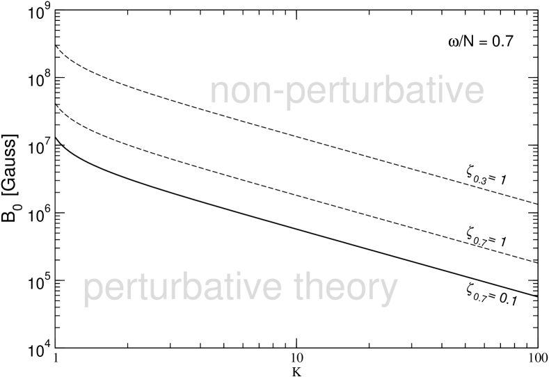
We consider the perturbative regime for magnetic fields, where , so that and MHD resonances () do not appear within the RZ. This region is the lower one in Fig. 2. The dashed curves labelled and correspond to resonances that occur at and in the non-perturbative region. The solid curve is chosen to illustrate the separation between the two regimes, according to the criterion . The perturbative magnetic field for which the maximum Alfvén velocity is small, , obeys
| (21) |
The absence of MHD resonances allows us to set
and thus derive from Eq. (3) the -correction to Eq. (19):
| (22) |
here the wave number correction is given by
Introducing the notation:
| (23) |
one gets from Eq. (22):
and after the change this equation takes the form
| (24) |
The general solution of Eq. (24) is expressed via the Bessel functions of the first kind, (see Gradstein & Ryzhik (2000)), and are constants. Now, coming back to the variable , we use the boundary condition at the solar center, (), to obtain the solution of Eq. (24) in RZ, ,
| (25) |
In CZ the Brunt-Väisälä frequency vanishes, , so that we are led to the same solution as in isotropic case , neglecting the possible existence of a CZ magnetic field (if such a field is present, with strength of 300 kG, the g-mode frequencies change by no more than ). Since the arguments of Bessel functions in Eq. (24) are small, we can use the first terms in the Bessel function series only,
| (26) |
Then by matching the logarithmic derivatives of the solutions and at the top of RZ, , one obtains the generalized dispersion equation for the case :
| (27) |
where .
This is our main equation. Clearly, when the magnetic field correction tends to zero, hence tends to , one recovers the isotropic case, given in Eq. (20).
We search for a perturbative solution of Eq. (3.2) of the form and where and correspondingly are the solution of Eq. (20) for and the smallness of and follows from .
The g-mode spectra for fixed kG are shown on Fig. 1 (see dashed curves). Figs. 3 and 4 display our results for as a function of mode radial order , magnetic field and wave number . One sees that the magnetic field shift of a g-mode frequency is always positive, . In Fig. 3 we show the absolute values of the shift for different g-modes and for fixed kG as a function of . Conversely, in Fig. 4 we fix the wave number and plot as a function of . One sees that, the higher the mode radial order , the less the magnetic field strength required to produce a given g-mode frequency shift.


4 Discussion
We have given a generalization of helioseismology to account for the presence of central magnetic fields in the Sun. We have determined the resulting g-mode spectrum within the framework of a perturbative one–dimensional Magneto-Hydrodynamics model.
There are three factors influencing g-mode observation in helioseismic experiments. First, such g-modes should have long wave lengths to penetrate the CZ: in our case , and in the 3D-model, low values of . Second, the radial order should also be low, otherwise, such low frequency g-modes are much below the present experimental sensitivity. Third, there is a strong influence of the RZ magnetic field.
If the magnetic field is too strong (more than a few MG) all g-modes are locked within the Alfvén cavity (see Burgess et al. (2004a)), hence these g-modes decay far beneath the CZ becoming invisible in the photosphere. This happens because the MHD energy in the radial direction is fully diverted to the transversal plane at the Alfvén resonant layer position. On the other hand, for very small magnetic fields ( MG) the magnetic field effect is negligible and can not account for a possible discrepancy between present experimental data and theoretical predictions of seismic models. In contrast, we have shown that a solar radiative zone magnetic fields of intermediate magnitude, of the order 600-800 kG, can displace the pure g-mode frequencies by about 1% with respect to our model of seismic wave propagation, a value close to what is hinted by results of the GOLF experiment.
We find that higher modes require a smaller magnetic field to produce a given g-mode frequency shift. However encouraging this result may sound, let us stress again that in our simple one-dimensional MHD picture (with further assumptions, such as adiabatic oscillations, exponential density profile, constant gravity, etc) we can only make a qualitative estimate of the magnetic field corrections to the pure g-mode spectrum. For example, our formalism can not explain the magnetic splitting of g-mode frequencies over azimuthal number , as it requires 3-D. Further work in 3-D geometry is necessary to perform a quantitative comparison with the frequency patterns observed in the GOLF experiment (Turck-Chièze et al., 2004). Even within the simple analytic approach 1-D MHD model one may include viscosity effects in non-ideal plasma with finite conductivity, and also take into account magnetic field diffusion stabilizing MHD instabilities.
Last, but not least, recall that our perturbative analysis avoids the appearance of MHD resonances that could lead to density spikes. These are potentially important, as they can affect neutrino propagation through the solar RZ (Burgess et al., 2003, 2004a, 2004b). Improved determination of neutrino mixing parameters, e.g. by KamLAND (Eguchi et al., 2003), allows one to carry out neutrino tomography in deep solar interior. Both regimes of “magnetized helioseismology” (i) the MHD seismic models and (ii) the analysis of MSW neutrino oscillations in noisy Sun are complementary tools to explore RZ magnetic fields. A fully quantitative analysis may require the inclusion of the differential rotation in the RZ (Turck-Chièze et al., 2005) as well as non-linearities.
Note added: As this paper was being typed, we saw a paper by Hasan, Zahn, & Christensen-Dalsgaard (2005) (astro-ph/0511472), where a similar idea to probe the internal magnetic field of slowly pulsating B-stars through g modes is given. Their 3-D results are consistent with our simpler 1-D estimates.
Acknowledgments
Work supported by Spanish grant BFM2002-00345. We thank N. Dzhalilov, M. Ruderman and S. Turck-Chièze for discussions. TIR and VBS thank IFIC’s AHEP group for hospitality during part of this work. They were partially supported by RFBR grant 04-02-16386 and the RAS Presidium Programme “Solar activity”. TIR was supported by a Marie Curie Incoming International Fellowship of the EC.
References
- Bahcall (1988) Bahcall, J.N., 1988 Neutrino Astrophysics, Cambridge University Press
- Burgess et al. (2003) Burgess, C.P. et al., 2003 , ApJ, 588, L65
- Burgess et al. (2004a) Burgess, C.P. et al., 2004a, MNRAS, 348, 609
- Burgess et al. (2004b) Burgess, C.P. et al., 2004b, JCAP, 01, 007
- Christensen-Dalsgaard (2003) Christensen-Dalsgaard, J., 2003, Lecture Notes on Stellar Oscillations, p. 145, available at http://astro.phys.au.dk/~jcd/oscilnotes/
- Hasan, Zahn, & Christensen-Dalsgaard (2005) Hasan, S.S., Zahn, J.-P., & Christensen-Dalsgaard, J. 2005, A&A, 444, L29
- Couvidat, Turck-Chièze & Kosovichev (2003) Couvidat, S., Turck-Chièze, S., Kosovichev, A.G., 2003, ApJ, 599, 1434
- Eguchi et al. (2003) Eguchi, K., et al. 2003, Phys. Rev. Lett., 90, 021802
- Gradstein & Ryzhik (2000) Gradshteyn I., Ryzhik I., 2000, Table of Integrals, Series, and Products 6-th Ed., Academic Press, p. 922, Eq. 8.492.1
- Kitchatinov, Jardine & Collier-Cameron (2001) Kitchatinov, L.L., Jardine, M., & Collier-Cameron, A. 2001, A&A, 374, 250
- Landau & Lifshitz (2000) Landau, L.D., & Lifshitz, E.M. 2000 Quantum Mechanics (Non-relativistic Theory), ed. Butterworth, Heineman
- Miles, Allen & Roberts (1992) Miles, A.J., Allen, H.R., & Roberts, B. 1992, Solar Physics, 141, 235
- Moss (2003) Moss, D. 2003, A&A, 403, 693
- Ruderman, Hollweg & Goossens (1997) Ruderman, M.S., Hollweg, J.V., & Goossens, M. 1997, Phys. Plasmas, 4, 75
- Ruzmaikin & Lindsey (2002) Ruzmaikin, A., & Lindsey, C. 2002, in Proceedings of SOHO 12/GONG + 2002 “Local and Global Helioseismology: The Present and Future”, Big. Bear Lake, California (USA)
- Turck-Chièze et al. (2004) Turck-Chièze, S., et al. 2004, ApJ, 604, 455
- Turck-Chièze et al. (2005) Turck-Chièze, S., et al. 2005, astro-ph/0510854