Sky coverage of orbital detectors. Analytical approach

Abstract

Orbital detectors without pointing capability have to keep their field of view axis laying on their orbital plane, to observe the largest sky fraction. A general approach to estimate the exposure of each sky element for such detectors is a valuable tool in the R&D phase of a project, when the detector characteristics are still to be fixed. An analytical method to estimate the sky exposure is developed, which makes only few very reasonable approximations. The formulae obtained with this method are used to compute the histogram of the sky exposure of a hypothetical gamma-ray detector installed on the ISS. The C++ code used in this example is freely available on the https://github.com/dcasadei/SkyCoverage web page.

1 Introduction

In addition to the large, complex and very expensive orbiting observatories, smaller size and lower cost detectors, whose goals are restricted to a narrower field, can perform interesting astrophysical measurements. To be (relatively) cheap, a satellite cannot have special pointing capabilities, beyond the normal gyroscopic stabilization and control, which is necessary not to loose communication with Earth stations and to keep safe satellite orientation.

When trying to define what are the parameters which should characterize an orbiting detector, one would like to be able to get values which are good estimations of the final parameters much before developing a complete Monte Carlo simulation. As an example, let us consider a detector which aims to measure the cosmic gamma-ray background in a wide energy range: its design acceptance and the mission duration will depend on the expected flux of known sources, in addition to the detector energy resolution.

To estimate the detector field of view and sensitive area, together with the mission duration, one needs to know the measured flux (per energy bin) coming from each sky element, which depends on the sources and on the detector characteristics. Thus, one will first produce the histograms of the sky exposure for different mission durations and then will consider different sensitive areas (i.e. different detector configurations), in order to find the configuration which best matches the expected fluxes.

Another case in which a method to determine the sky exposure for a given detecor can be very useful is when one tries to understand the possible performance of an existing detector for the search for a new “channel” in the data analysis, and the access to the detailed simulation software is not easy, fast, or allowed. If the obtained values suggest the possibility of doing interesting astrophysics, one will of course use the official detector simulation program to refine the estimation.

In this paper, an analytical method to obtain the sky coverage of an orbiting detector is shown, which makes use of few reasonable assumptions to simplify the computation: (1) the orbit eccentricity is zero; (2) the orbit precession period is much larger than the revolution period; (3) the detector field of view is a cone, whose axis lies in the orbital plane, rotating with the same angular velocity of the satellite revolution. These assumptions are valid in the case of a detector installed on the International Space Station (ISS), taken as an example in the following sections. A program has been developed which makes use of this method: its C++ code is freely available on the http://cern.ch/casadei/software.html web page.

2 The method assumptions and algorithm

2.1 Hypotheses

The first hypothesis (null eccentricity $e$) implies that the revolution velocity is constant. Its explicit dependence on the orbit parameters is shown in ref. [1]: the result is a function with a rather weak dependence on $e$, hence this approximation is quite good for small values of $e$.

The second hypothesis (orbit precession period $T\gg\tau$, where $\tau$ is the revolution period) is valid in general, and allows for a useful approximation: the method first computes the sky exposure over a single orbit, then rotates this map following the orbit precession.

The hypothesis that the field of view is a cone with axis in the orbital plane is not true in general. The real detector acceptance is usally different from a uniform cone, though one often accepts tracks within some “fiducial” cone to make easier the off-line data analysis (avoiding “border effects”). Having the axis contained in the orbital plane maximizes the fraction of the sky seen by the detector, hence it is a quite natural choice. Finally, having angular velocity equal to that of the revolution motion means that the angle (in the orbital plane) between the cone axis and the radial vector (from the orbit center to the satellite) is kept constant. This is true for detectors installed on the ISS.

The detector acceptance will in general depend both on the incident angle $\alpha$ of the photon and on its energy, with $\alpha=0$ for tracks parallel to the cone axis. However, we neglect this angular dependency and consider a uniform acceptance in $\alpha$ inside a cone with half-aperture $\alpha_{\mathrm{c}}$. The analytical method presented here is really fast from the computing point of view, and it is easy to change the source code to implement the effect of the $\alpha$ dependence of the acceptance (only a single file needs to be changed). On the other hand, it will be much more tricky to implement the azimuthal dependence of the detector acceptance: if the user really needs to reach this level of detail, she/he would benefit from switching to the official detector simulation.

2.2 Reference systems

In this paper, three reference systems are used: the orbit reference system (hereafter ORS), the galactic reference system (GRS), and the precession reference system (PRS). The GRS is the system in which we usually want to express the results. The PRS is used as intermediate step by the algorithm, to simplify the precession computation. Finally, the equatorial $(x,y)$ plane of the ORS is the plane of the orbit. PRS and GRS are inertial reference sytems (they do not rotate).

Because we will consider here only mission durations which are at least few times longer than the precession period, the exact position of the detector when it starts data taking is not important. Hence, we are only interested in the orbit unit vector $\hat{\boldsymbol{n}}$, which defines the $z$ axis in the ORS. The $(x,y)$ plane is the orbital plane in this reference system, and we are free to choose the axes direction in ordert to simplify the computation.

A possible choice for the reference axes $(X,Y,Z)$ in the GRS is the following. The axes are defined by the three unit vectors $\hat{\boldsymbol{I}}$, $\hat{\boldsymbol{J}}$ and $\hat{\boldsymbol{K}}$ respectively: $\hat{\boldsymbol{I}}$ points to the vernal equinox direction, $\hat{\boldsymbol{K}}$ to the North Pole and $\hat{\boldsymbol{J}}$ completes the right-handed triplet [1]. Any point in the sky can be addressed in the GRS using two angles: $\Theta\in[0,\pi]$, which is the angle formed with $\hat{\boldsymbol{K}}$, and $\Phi\in[0,2\pi]$, expressing the rotation in the equatorial $(X,Y)$ plane, starting from the $\hat{\boldsymbol{I}}$ unit vector. Astronomers usually adopt the “equatorial coordinates” declination $\delta=\pi/2-\Theta$ and right ascension $\alpha=\Phi$ instead of $\Theta$ and $\Phi$. However, using the colatitude $\Theta$ instead of $\delta$ simplifies the histogramming.

The orbit precession is described by the constant unit vector $\hat{\boldsymbol{k}}$ about which the orbit normal $\hat{\boldsymbol{n}}$ rotates while keeping $\hat{\boldsymbol{k}}\boldsymbol{\cdot}\hat{\boldsymbol{n}}(t)=\cos\beta$ constant. The $\hat{\boldsymbol{k}}$ unit vector defines the $z^{\prime}$ axis of the PRS, and we are free to choose the direction of the $x^{\prime}$ and $y^{\prime}$ axes to simplify the computation. The algorithm needs the PRS when computing the orbit precession effect on the sky exposure map, which in the PRS is simply a rotation around $\hat{\boldsymbol{k}}$ of the histogram obtained for a single orbit.

2.3 Algorithm

For each sky element, its exposure is equal to the product of its solid angle and the total time for which it is found inside the detector acceptance. During few orbits, as long as $\,\mathrm{d}\hat{\boldsymbol{n}}/\,\mathrm{d}{t}$ can be neglected, the same points are seen by the detector few times: if $\alpha_{\mathrm{c}}<90$ deg (as usual), the celestial sphere is divided in two parts by the “belt” viewed by the detector. The exposure is largest for points situated along the central part of the belt, and decreases to zero going from the center to the boundaries.

After a large number of orbits, the precession of the belt increases the sky fraction viewed by the detector. For each sky element, its exposure is equal to the convolution between the time spent inside the belt (which rotates following the orbit precession) and the exposure function inside the belt (computed along one revolution).

The algorithm, for the case in which the detector acceptance is uniform inside a cone with half-aperture $\alpha_{\mathrm{c}}$ whose axis is defined as the detector axis, is based on the following ideas:

1. to find the exposure map of the sky in the ORS for one revolution, we will follow an analytical treatment (section 3);

2. the (slow) orbit precession in the PRS is computed with a discrete algorithm acting on the exposure histogram (section 4.1);

3. the exposure map of the sky in the GRS is found analytically (section 4.2).

If the real detector acceptance does not have cylindrical symmetry, one has first to compute the real belt exposure along one orbit by changing step 1 (i.e. by changing a single C function in the code), and then can proceed as before. When considering the dependence of the acceptance on the photon energy, one will repeat the three steps independently in each energy bin.

3 Single orbit exposure map

Figure 1: Sky sphere viewed by a cone.

Let the detector field of view be a cone of half-aperture $\alpha_{\mathrm{c}}$ (figure 1), with axis along the unit vector $\hat{\boldsymbol{r}}$ (the “local vertical”). The latter turns around $\hat{\boldsymbol{n}}$ with angular velocity $\omega=2\pi/\tau$, and instant velocity unit vector $\hat{\boldsymbol{v}}=\hat{\boldsymbol{n}}\boldsymbol{\times}\hat{\boldsymbol{r}}$ (the “local horizontal”).

3.1 Sky coverage in the orbit reference system

All points along the $\hat{\boldsymbol{r}}$ trajectory are inside the cone for a time $t=2\alpha_{\mathrm{c}}/\omega=\alpha_{\mathrm{c}}\tau/\pi$ during each orbit. The fraction of time during which a point P in the sky is found inside the cone depends on the angle $\alpha$ formed with the equatorial plane (which contains $\hat{\boldsymbol{r}}$ and $\hat{\boldsymbol{v}}$). This time $t(\alpha)$ is maximum when $\alpha=0$ and goes to zero when $\alpha$ approaches $\alpha_{\mathrm{c}}$. For higher angles, the point is never contained by the cone (we restrict our analysis to $\alpha_{\mathrm{c}}<90$ deg).

The “parallel” passing through P is a circumference with length $\ell=2\pi R\cos\alpha$ (figure 3). Let $\psi$ be the half angular width of this parallel, when projected to the equatorial plane (figure 3): when $\alpha$ approaches $\alpha_{\mathrm{c}}$, $\psi$ goes to zero; as $\alpha$ goes to zero, $\psi$ approaches $\alpha_{\mathrm{c}}$. The exposure time $t(\alpha)$ is equal to the ratio between the parallel width $2\psi$ and the angular velocity:

$$t(\alpha)=\frac{2\,\psi(\alpha)}{\omega}=\frac{\tau}{\pi}\,\psi(\alpha)\;.$$ (1)

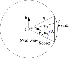
Figure 2: Side view of the sky sphere.

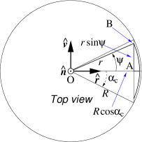
Figure 3: Top view of the sky sphere.

In order to find $\psi(\alpha)$, we consider the triangle ABO on the equatorial plane (see figure 3) and observe that the segment BO, the radius of the parallel passing through P, is $r=R\cos\alpha$. The lengths of the segments AO and AB are $R\cos\alpha_{\mathrm{c}}$ and $r\sin\psi$ respectively. The Pitagora’s theorem implies that

$$\cos^{2}\alpha=\cos^{2}\alpha_{\mathrm{c}}+\cos^{2}\alpha\sin^{2}\psi\;,$$ (2)

hence one finds that $\sin\psi$ can be written as:

$$\sin\psi=\sqrt{1-\frac{\cos^{2}\alpha_{\mathrm{c}}}{\cos^{2}\alpha}}\;.$$ (3)

One can easily verify that this expression has the expected behavior when $\alpha$ approaches zero or $\alpha_{\mathrm{c}}$.

Finally, the time $t(\alpha)$ during which the point P, seen at the angle $\alpha$ with respect to the equatorial plane, is viewed by the detector is:

$$t(\alpha)=\frac{\tau}{\pi}\,\arcsin\!\sqrt{1-\frac{\cos^{2}\alpha_{\mathrm{c}}}{\cos^{2}\alpha}}\;,$$ (4)

with $-\alpha_{\mathrm{c}}\leq\alpha\leq\alpha_{\mathrm{c}}$ (see figure 4, where $\alpha_{\mathrm{c}}=25$ deg).

A better choice of the angle is the orbital colatitude $\theta=\frac{\pi}{2}-\alpha$ (also shown in figure 4): for any direction $\hat{\boldsymbol{d}}$ in the sky one has $\hat{\boldsymbol{n}}\boldsymbol{\cdot}\hat{\boldsymbol{d}}=\cos\theta$. Every sky element can be mapped using $\theta$ and the angle $\phi$ of rotation about $\hat{\boldsymbol{n}}$: the solid angle element centered on $\hat{\boldsymbol{d}}$ is $\,\mathrm{d}\Omega=\sin\theta\,\mathrm{d}\theta\,\mathrm{d}\phi$ and its exposure per orbit is $t(\hat{\boldsymbol{d}})\,\mathrm{d}\Omega$, i.e.:

$$t(\hat{\boldsymbol{d}})\,\mathrm{d}\Omega=\dfrac{\tau}{\pi}\,\arcsin\!\sqrt{1-\dfrac{\cos^{2}\alpha_{\mathrm{c}}}{\sin^{2}\theta}}\,\sin\theta\,\mathrm{d}\theta\,\mathrm{d}\phi$$ (5)

for $(\frac{\pi}{2}-\alpha_{\mathrm{c}})\leq\theta\leq(\frac{\pi}{2}+\alpha_{\mathrm{c}})$ and $t(\hat{\boldsymbol{d}})\,\mathrm{d}\Omega=0$ otherwise. In the following, we will omit to recall that the exposure is zero when the condition $(\frac{\pi}{2}-\alpha_{\mathrm{c}})\leq\theta\leq(\frac{\pi}{2}+\alpha_{\mathrm{c}})$ is not satisfied.

Figure 4: Fractional exposure time (in units of the orbit period $\tau$) of a cone with $\alpha_{\mathrm{c}}=25$ deg, as function of the angles $\alpha$ and $\theta$.

In numeric computations, given the partition of the sky in elements $\Delta\Omega=\Delta(\cos\theta)\,\Delta\phi$, corresponding to uniform binning in $\phi$ and $\cos\theta$, one can produce the exposure histogram using equation (5), which can be rewritten as:

$$t(\hat{\boldsymbol{d}})\,\Delta\Omega=\frac{\tau}{\pi}\,\arcsin\!\sqrt{1-\frac{\cos^{2}\alpha_{\mathrm{c}}}{1-\cos^{2}\theta}}\,\Delta\phi\,\Delta(\cos\theta)\;,$$ (6)

where $\cos\theta$ is the central value of the considered bin, whose width is $\Delta(\cos\theta)$.

3.2 Sky coverage in the precession reference system

Equation (6) is valid in any $(x,y,z)$ reference system where $\hat{\boldsymbol{n}}$ is the unit vector defining the $z$-axis. In order to compute the effect of the orbit precession, we move from the ORS to the $(x^{\prime},y^{\prime},z^{\prime})$ PRS with a rotation about the $x=x^{\prime}$ axis:

$$\mathsf{A}=\left(\begin{matrix}1&0&0\\ 0&\cos\beta&\sin\beta\\ 0&-\sin\beta&\cos\beta\\ \end{matrix}\right)\;.$$ (7)

In the PRS the orbit precession simply results in a drift along $\phi^{\prime}$ ($\phi^{\prime}=0$ along the $x^{\prime}$ direction, increasing following the orbital motion) of the sky elements in the $\cos\theta^{\prime}$ vs. $\phi^{\prime}$ exposure histogram (i.e. in a horizontal shift of the column contents). We consider the sky element $\Delta\phi^{\prime}\Delta(\cos\theta^{\prime})$ centered around the direction which can be written in Cartesian coordinates as

$$\begin{cases}x^{\prime}=\sin\theta^{\prime}\cos\phi^{\prime}\\ y^{\prime}=\sin\theta^{\prime}\sin\phi^{\prime}\\ z^{\prime}=\cos\theta^{\prime}\\ \end{cases}\;.$$ (8)

To apply equation (6), which is independent of $\phi$, we only need to find $z=\cos\theta$ by applying $\mathsf{A}^{-1}$, obtaining:

$$\cos\theta=z=\sqrt{1-\cos^{2}\theta^{\prime}}\sin\phi^{\prime}\sin\beta+\cos\theta^{\prime}\cos\beta\;.$$ (9)

Using equation (9) together with (6), one can obtain a histogram similar to figure 5, which shows the sky exposure map (for one orbit, in units of the revolution period) seen by a detector whose field of view is a cone with half aperture 25 deg, installed on the ISS: in the PRS, the “belt” is inclined of 51.6 deg, which is the ISS orbit inclination.

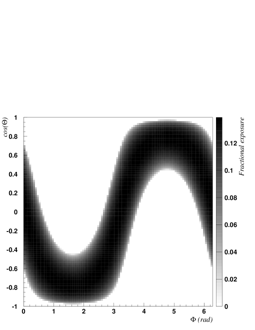
Figure 5: Single orbit exposure map per unit period, for a detector with field of view of 50 deg (25 deg is the cone half aperture), orbiting on board of the the ISS. The ExposureFraction histogram size is $100\times 100$ bins.

In the following, we will illustrate the method by choosing a mission duration $T_{\text{mi}}=1000$ days and the detector axis to be parallel to the ISS local vertical. These parameters are similar (though not identical) to those of the AMS-02 detector [2], which will be installed on the ISS in the near future. The ISS orbit parameters are approximated as follows: the revolution period $\tau\simeq 1.5$ h, the precession period $T_{\text{pr}}\simeq 2$ months. With altitudes in the range 350–400 km above sea level, the orbit eccentricity $e=6.55\times 10^{-4}$ is very small (i.e. our first hypothesis is good). In addition, the ISS attitude is controlled in order to keep its local vertical axis parallel to the radial vector (hence the third hypothesis is also good).

4 Orbit precession

Let us call ExposureFraction the histogram representing the “belt” in the PRS (figure 5), and PrsSkyMap the histogram of the exposure in the PRS, which we have now to fill. The bin contents of ExposureFraction are pure numbers: they must be multiplied by the orbit period $\tau$ to obtain the exposure of each $\Delta\Omega$ sky element during a single orbit.

4.1 Orbit precession in the precession reference system

To fill the PrsSkyMap histogram, which has $N_{\phi}$ bins in $\phi^{\prime}$ and $N_{\theta}$ bins in $\cos\theta^{\prime}$, we have to compute the effects of the orbit precession, which in the PRS results in a drift along $\phi^{\prime}$ of the sky elements obtained using equation (6) after the substitution (9). The algorithm is the following.

1. One has first to compute the time required for the orbit precession to move each bin on top of the following one. This time is $t_{\phi}=T_{\text{pr}}/N_{\phi}$, with $T_{\text{pr}}=2$ months is the precession period.

2. Given the mission duration $T_{\text{mi}}$, one has to find the number of times the $\phi$ bins have to be rotated, which is $N_{\text{ro}}=T_{\text{mi}}/t_{\phi}$.

3. Then one has to performs $N_{\text{ro}}$ iterations which consist of a loop over the $N_{\phi}$ columns, whose single step is the sum of the ExposureFraction $(i-1)$-th column contents to the PrsSkyMap $i$-th column (with $i$ decreasing from $N_{\phi}$ to 1). Of course, the last column should be added to the first one.

4. Finally, to get the exposure time for each $\Delta\Omega$ sky element, one has to multiply each PrsSkyMap bin by the revolution period $\tau$.

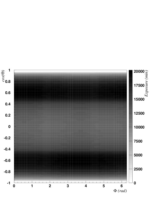
Figure 6: Exposure (in minutes) in the PRS of a detector with field of view of 50 deg (25 deg is the cone half aperture), orbiting on board of the the ISS. The orbit period is 90 min, the precession period is 2 months, and the mission duration is 1000 days. The PrsSkyMap histogram size is $100\times 100$ bins.

Figure 6 shows the result for our hypothetical detector on the ISS. The PrsSkyMap histogram has $100\times 100$ bins.

4.2 Orbit precession in the galactic reference system

The histogram GrsSkyMap representing the sky map in the GRS can be filled with the assumption that the $\Phi$-granularity of GrsSkyMap should be identical to the $\phi^{\prime}$-granularity of PrsSkyMap (which is quite reasonable). However, one can not find the PRS histogram and then transform it to the GRS map, because continuous transformations can not be applied to discretized maps without introducing distortions. Then the procedure is the following.

For each GrsSkyMap bin, relative to the direction $\hat{\boldsymbol{d}}$ corresponding to the coordinates $(\Phi,\cos\Theta)$ of the bin center, we need to find the PRS coordinates which represent the same direction:

$$\hat{\boldsymbol{d}}_{\text{PRS}}\equiv(\phi^{\prime}(\Theta,\Phi),\,\cos\theta^{\prime}(\Theta,\Phi))\equiv(\phi^{\prime}_{j},\,\cos\theta^{\prime}_{i})\;,$$ (10)

where $i\in[0,N_{\theta}-1]$ and $j\in[0,N_{\phi}-1]$ are the row and column indices, respectively, of the PrsSkyMap bin which contains $\hat{\boldsymbol{d}}_{\text{PRS}}$.

Each $\phi^{\prime}$-bin (and $\Phi$-bin, for the previous assumption) is $\Delta\phi^{\prime}=2\pi/N_{\phi}$ wide and is inside the detector field of view for a time $t_{\phi}$ per orbit. In the PRS, the time $T(\hat{\boldsymbol{d}})$ spent inside this bin is the sum over $N_{\text{ro}}$ rotations of the PrsSkyMap columns, due to the orbit precession. Hence

$$T(\hat{\boldsymbol{d}})=\sum_{k=0}^{N_{\text{ro}}-1}\arcsin\sqrt{1-\frac{\cos^{2}\alpha_{\mathrm{c}}}{1-F_{k}(\theta^{\prime},\phi^{\prime})}}$$ (11)

with

$$F_{k}(\theta^{\prime},\phi^{\prime})=\cos^{2}\theta(\theta^{\prime}_{i},\phi^{\prime}_{j}-k\Delta\phi^{\prime})=\cos^{2}\theta(\theta^{\prime}_{i},\phi^{\prime}_{j(k)})$$ (12)

where $j(k)$ is the $\phi^{\prime}$-bin which contains $\phi^{\prime}_{j}-k\Delta\phi^{\prime}$. Finally, to obtain the total exposure in the considered GrsSkyMap bin, we have to multiply the time spent viewing each sky portion centered around $(\Phi,\cos\Theta)$ for $N_{\text{ro}}$ times its solid angle: the result is $N_{\text{ro}}T(\hat{\boldsymbol{d}})\Delta\Omega$, where $T(\hat{\boldsymbol{d}})$ is given by the formula (11).

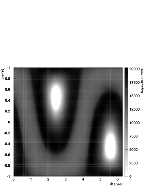
Figure 7: Exposure (in minutes) in the GRS, after an Euler’s rotation of angles (-33, 62.6, -77.75) deg.

Actually, the real algorithm follow by the program starts from the GrsSkyMap histogram and loops over its bins. For each bin in the GRS, it finds the corresponding bin in the PRS using an Euler’s rotation, then applies formula (11). Figure 7 shows the final result, after a rotation with Euler’s angles of (-33, 62.6, -77.75) deg. The first angle is the rotation about the third axis, which transform the first axis in the ‘line of nodes’. The second angle is a rotation about the line of nodes, which moves the third axis in the final position. The third angle is a rotation about the new third axis, which transforms the line of nodes into the final first axis. In order to show another possible choice of the coordinate system, we considered the PRS as the celestial-equatorial reference system in our example, and chose the Euler’s angles which transform it to the GRS, expressed in the B1950.0 epoch as defined in 1958 by the IAU [3].

5 Detector sensitivity

Having obtained the exposure time of each sky element, the detector sensitivity is found in the following way. The first step is to compute the product of the effective detector sensitive area $A(E)$ (usually expressed in cm²) with the sky element exposure $\Delta\Omega\,t$ (sr s):

$$S(E)=A(E)\,\Delta\Omega\,t\quad(\!\,\mathrm{cm^{2}}\,\mathrm{sr}\,\mathrm{s})\;.$$ (13)

The effective area $A(E)$ in general will depend on the photon energy $E$ and on the incident direction. Here we consider a uniform acceptance over all directions inside the field of view, hence our expression for $S(E)$ is equivalent to the average over all directions of the real detector efficiency.

If a known source, covering the sky element $\Delta\Omega$ (which can be contained in a single histogram bin or extend over a set of adjacent bins), has a photon flux $F(E)$ $(\!\,\mathrm{cm^{-2}}\,\mathrm{sr^{-1}}\,\mathrm{s^{-1}})$ in a particular energy bin centered at $E$, then the number of events measured by the detector are expected to be:

$$N_{\text{meas}}(E)=F(E)\,S(E)\;.$$ (14)

On the other hand, there will be some background flux of photons coming from the same sky element, which will produce background events in each energy bin. Formula (14) can also be used to find the number of expected background hits in the detector. In case one considers a single energy bin, she/he would define the detector source sensitivity in this bin as the ratio between the number of expected measured events and the square root of the number of background hits, or follow the more detailed approach of ref. [4]. However, the usual approach is to consider the whole detector energy range at the same time, and to perform a fit of the measured distribution (deconvolved with the detector sensitivity) with a function which is modeling both the source spectrum and the background flux at the same time.

In this way, for each set of detector parameters, it is possible to identify the sources which are visible with the considered orbit and mission duration.

6 Conclusion

The analytical method developed in this paper allows for a fast estimation of the detector sensitivity to known sources, when the hypotheses considered in section 2 are valid. The source code, freely available on the author’s web site, is a useful tool during the design phase of an experiment making use of an orbital detector, when the goal is the definition of its parameters and of the mission duration. In addition, it is useful also as a way to easily check the performance of existing detectors, when access to their detailed simulation program is not easy or allowed.

On the other hand, if one really needs a precise estimation of the detector performance, she/he would need to make use (or to develop) a program which exactly tracks the satellite along its orbital motion using complicated formule, which can be found in papers like ref. [1] or textbooks like ref. [5] and [6]. In addition, the program should be able to correctly simulate the detector response to photons with different energies and incident directions, as was done for example by the AMS collaboration [7, 8, 9, 10]. But the price for the higher precision is a CPU intensive and complex program (with usually harder user interface than this analytic method), and a long development time.

References

- [1] A. Murad, et al., A Summary of Satellite Orbit Related Calculations, Tech. Rep. 95-12, CSHCN, (ISR T.R. 95-107) (1995).
- [2] M. Aguilar, et al., Phys. Rep. 366/6 (2002) 331–404.
- [3] M. Zombeck, Handbook of Astronomy and Astrophysics, Second Edition, Cambridge University Press, Cambridge, UK, 1990.
- [4] Ti-Pei Li & Yu-Qian Ma, ApJ 272 (1983) 317–324.
- [5] J. Wertz (Ed.), Spacecraft Attitude Determination and Control, no. 73 in Astrophysics and space science library, Kluwer Academic Publishers, 1978.
- [6] A. Roy, Orbital Motion, Adam Hilger, Bristol, 1988.
- [7] S. Natale, Gamma Sources Analysis, AMS Gamma Meeting, CERN, Dec. 13, 2001 (2001).
- [8] I. Sevilla Noarbe, Simulation of the Orbit of AMS on-board the International Space Station, AMS Internal Note 2004-03-03 (2004).
- [9] A. Jacholkowska, et al., An indirect dark matter search with diffuse gamma rays from the Galactic Centre: prospects for the Alpha Magnetic Spectrometer, astro-ph/0508349 (2005).
- [10] G. Valle, A&A 424 (2004) 765–772.