Troubles for observing the inflaton potential

Abstract

Robustness of the solutions to the inflaton potential inverse problem based on the slow-roll approximation is addressed. With that aim it is introduced a measure of the difference of the outputs obtained using first and second order respectively in the horizon-flow expansion. The evolution of this measure is determined by a second order linear non-autonomous non-homogeneous differential equation. Boundedness of the general solutions to this equation is analyzed. It is shown that they diverge for most of the physically meaningful cases. Examples for typical inflationary models are presented. It is argued that this lack of robustness is due to the limitations of the slow-roll expansion for probing the scale-dependence of the inflationary spectra.

Keywords: inflation, CMBR, slow-roll, inflaton potential

1 Introduction

The relatively recent release of the analysis of the first year WMAP data [1] and of a significant amount of very precise data of the power spectrum of matter distribution at large scales [2] caused a turmoil in the cosmological community. The feasibility of obtaining reliable information about our universe when it was younger than $10^{-10}$ seconds accounts for a large part of that excitement. Data confirmed that the primordial power spectrum of curvature fluctuations is consistent with a scale-invariant, Gaussian and adiabatic spectrum. The simplest and most elegant mechanism known to causally produce primordial spectra with those properties is cosmological inflation.

In the simplest scenarios with an exit from inflation the responsible for the accelerated expansion of the early Universe is the inflaton $\varphi$, a single scalar field with equations of motion,

$$\ddot{\varphi}+3H\dot{\varphi}+V^{\prime}(\varphi)=0\,,$$ (1)

$$H^{2}=\frac{1}{3}\left[\frac{\dot{\varphi}^{2}}{2}+V(\varphi)\right]\,.$$ (2)

Here $V(\varphi)$ is the potential energy density of the inflaton field, dot stands for a derivative with respect to cosmic time $t$, and prime denotes a derivative with respect to $\varphi$. We use Planck units, $8\pi G=c=\hbar=1$.

The Hubble horizon $d_{\rm H}\equiv 1/H$, is roughly the size of the region where causal processes can take place during one Hubble time $1/H$. During inflation the comoving $d_{\rm H}$ decreased allowing comoving scales to cross out the causal horizon. Physical information of the inflaton and of the space-time quantum fluctuations contained on those scales was effectively ‘frozen’. This way, when the scales crossed $d_{\rm H}$ back later during the era of standard (non-accelerated) expansion, the whole observable universe was seed with statistically uniform curvature perturbations for large-scale structure formation. These seeds served also as initial conditions for the evolution of CMBR anisotropies.

The spectra of quantum fluctuations of density and metrics during cosmological inflation can be predicted [3]. It is required to know the behavior of the Hubble horizon as a function of the logarithm of the scale factor, $N\equiv\ln a(t)$. In the inflaton scenario it means solving Eqs.(1) and (2). For most potentials that is a difficult task that can be simplified using the horizon-flow functions which are defined recursively as [4]:

$$\epsilon_{m+1}\equiv{{\rm d}\ln|\epsilon_{m}|\over{\rm d}N}\quad\forall m\geq 0,\quad\epsilon_{0}={H(N_{\rm i})\over H(N)}\,,$$ (3)

where $N_{\rm i}$ denotes an arbitrary ‘initial’ moment. The necessary condition for inflation to take place is $\epsilon_{1}<1$, and if the weak energy condition and null energy condition hold true, $\epsilon_{1}\geq 0$. In general, for the primordial spectra to be nearly scale invariant, it is sufficient to assume $|\epsilon_{m}|<1$ allowing, this way, to expand all the interesting inflationary quantities in terms of the horizon-flow functions. The slow-roll approximation is a particular case where all the $\epsilon_{m}$ are assumed to have the same order of magnitude.

Eqs.(1) and (2) relate the horizon-flow functions to the inflaton potential $V(\varphi)$ and its derivatives with respect to the inflaton field. For instance, the first two flow functions are given approximately by [6]:

$$\epsilon_{1}\approx\frac{1}{2}\left(\frac{V^{\prime}}{V}\right)^{2}\,,\qquad\epsilon_{2}\approx 2\left[\left(\frac{V^{\prime}}{V}\right)^{2}-\frac{V^{\prime\prime}}{V}\right]\,.$$ (4)

In turn, the behavior of $d_{\rm H}(N)$ near a suitable pivot point $N_{*}$ is described by

$$d_{\rm H}(N) = d_{\rm H}(N_{*})\left[1+\epsilon_{1}(N-N_{*})+\frac{1}{2}(\epsilon_{1}^{2}+\epsilon_{1}\epsilon_{2})(N-N_{*})^{2}+\cdots\right]\,.$$ (5)

Thus, approximated expressions for the inflationary spectra can be derived. To first order for the horizon-flow functions they were found by Stewart and Lyth [7] using the slow-roll approximation to truncate the argument of Bessel functions evaluated at the time of horizon-crossing. Their accuracy was tested against numerical solutions in Refs. [8, 9, 5]. In the same approximation but using Green’s functions, second order expressions were derived in Refs. [10, 6] and tested by Schwarz and Terrero [9]. The approach based on Bessel functions was then modified [4, 9] to derive expressions at any order for two wide classes of inflationary models that do not necessarily satisfy the slow-roll condition. Up to third order, the corresponding expressions were tested in Ref. [9]. Several other methods were introduced to allow for relaxing the standard slow-roll condition [11, 12, 13]. In general, their predictions seem to match the accuracy of those methods tested against numerical results. All these tests yielded that the predictions of inflationary spectra using terms up to second order in the horizon-flow expansion are accurate enough to match the precision of current and near future observations.

This way, given an inflaton potential as input in Eqs.(1) and (2), the horizon-flow functions (3) can be evaluated at any moment, the behavior of the Hubble radius can be described by means of (5), the spectra of the inflaton and metrics fluctuations accurately predicted, used as initial conditions for the calculation of the evolution of scalar and tensor modes of anisotropies of the CMBR, and the resulting spectra compared with the observational data to test the reliability of the given inflationary model.

‘Observing’ the inflaton potential means solving the related inverse problem, i.e., that of looking for the functional form of the inflaton potential corresponding to given CMBR spectra. Herein, we will refer to this task as the Inverse Problem for the Inflaton Potential (IP²). Starting with the seminal paper by Hodges and Blumenthal [14], during the last 15 years there were introduced several methods for solving the IP². Depending on the way the output is given, they can be classified in parametric [14, 15, 16, 17, 18], perturbative [15, 19, 20], full-numerical [21], and stochastic [22] methods.

Assuming that the initial conditions for the calculation of CMBR spectra have been already fitted to the observational data, what all the methods for solving the IP² do (with the remarkable exception of the full-numerical method) is, essentially, to start by looking for the combinations of $\epsilon_{m}$ that gives the best fit to those primordial spectra. These combinations are constrained by the form and order of the approximated expressions for the spectra of density and metrics fluctuations. Note that, following definitions (3), the number $m$ of horizon-flow functions is directly related to the order of the corresponding expressions. In its turn, the order of the predicted spectra is constrained by the finite precision of data. Now, according with expansion (5), specifying the set $\{\epsilon_{m}(N_{*})\}$ is equivalent to specifying $d_{\rm H}(N)$. So, the unavoidable truncation of $\{\epsilon_{m}(N_{*})\}$ corresponds to an incomplete knowledge of the evolution of the Hubble horizon. The next step in the IP² solution is to use Eqs.(1) and (2), or the approximations (4), to find the functional form of the inflaton potential corresponding to that approximated behavior of $d_{H}(N)$.

The reliability of solving the IP² for a potential as constrained by measurement errors was directly tested in Refs. [20, 23]. There is also a large number of studies on the impact of the observational uncertainty on the form of the output potential. They give us complementary information about possible troubles for observing the potential (see Refs. [24, 6, 9, 25, 26, 27] and references therein). Though the results are in general encouraging, it must be noted that each of them uses in their analysis a fixed order for the slow-roll expansion of the primordial spectra. This is a formal expansion, hence there is not rigorous proof that it converges so, there is not certainty about the solution of the inverse problem based on this expansion to be robust. By robust we mean that, while increasing the order of the underlying expressions, the IP² solution must converge to a unique functional form. This robustness is required in order to make definite statements about the high energy physics linked to the observed inflaton potential.

In this sense, the preliminary analysis presented in Ref. [28] gave us a first cautionary warning about the possible existence of troubles for the robust solution of the IP² when the slow-roll approximation is used. The aim of this paper is to step forward in the analysis of the robustness of the reconstruction of the inflaton potential with regards to the convergence of the horizon-flow expansion for the spectra of inflationary perturbations under the slow-roll approximation. With that in mind, in the next section we will derive the basic equation for our analysis, a second order linear non-autonomous non-homogeneous differential equation obtained from the comparison between equations for the inflationary perturbations to first and second order in the horizon-flow expansion. In Sec.3 we will present mathematical evidence pointing to the non-existence of bounded solutions for this equation if the time variation of the coefficients is required to be consistent with the inflationary cosmology. We reinforce that conclusion in Sec.4, based on the analysis of inflationary models belonging to the prototypical classes introduced in Ref. [9]. Finally, in Sec.5 we discuss our results.

2 The basic equation

For finding the functional form of the inflaton potential all the methods mentioned in the Introduction use the same kind of expressions for the spectra of scalar perturbations. Nevertheless, early in the research on the IP² it was realized that the rôle of tensor perturbations deserves also attention if a unique solution to that problem is desired [23]. The information on these modes in the available data is so far rather poor [1, 2]. That is why all the studies but the so-called Stewart-Lyth inverse problem [18] avoided to deal with the tensor equations. However, the quality of the data on the tensor modes could be radically improved if a number of interesting experiments manages to see the primordial light (see for instances Refs. [29]). Even more, studies based on the parametric method have shown that even a poor information on the spectrum of the primordial gravitational waves allows for breaking the degeneracy in the solution of the IP² and for obtaining interesting results [30, 31, 32]. Particularly, in Ref. [32] it was shown how using the ratio of the amplitudes of the tensor and scalar perturbations,

$$r\equiv\alpha\frac{A_{T}^{2}}{A_{S}^{2}}\,,\qquad\left(\alpha=constant\right)\,,$$

as input for the IP² can be a very fruitful way of taking into account the available observational information on both types of spectra to observe the convexity of the potential during inflation. To do that it is necessary to solve the differential equation (recall the definitions (3) for the $\epsilon_{m}$),

$$\ln\frac{r}{r_{0}}=\ln\epsilon_{1}+C\epsilon_{2}+C_{1}\epsilon_{1}\epsilon_{2}+C_{2}\epsilon_{2}^{2}+C_{3}\epsilon_{2}\epsilon_{3}\,,$$ (6)

where $r_{0}$ is a constant and

$$C\approx-0.7296\,,$$ (7)

$$C_{1}\equiv\left(-\frac{\pi^{2}}{2}+5+C\right)\approx-0.6644\,,$$ (8)

$$C_{2}\equiv\left(-\frac{\pi^{2}}{8}+1\right)\approx-0.2337\,,$$ (9)

$$C_{3}\equiv\left(-\frac{\pi^{2}}{24}+\frac{C^{2}}{2}\right)\approx-0.1451\,.$$ (10)

This equation can be derived from the second order expressions for the amplitudes of the scalar and tensor perturbations obtained using the slow-roll approximation [10, 6]. (It can also be derived following the lines described in Ref. [32].)

If the reconstruction of the inflaton potential were robust, then we would expect that, given $r/r_{0}$ as input into the IP², the output using up to first order in Eq. (6) (see Ref. [32] for an example of such an output) will differ only in small features from the output of the problem with the same input but taking into account all terms in (6). To assess this small departure, following Ref. [28], we introduce a quantity $\delta(N)$ such that

$${}^{\rm s}\!\epsilon_{1}=\epsilon_{1}\left(1+\delta\right)\,,$$ (11)

where the ‘s’ denotes the horizon-flow functions in the set to be found if second order terms in Eq. (6) were used. The standard notation remains for the set found with up to first order terms. Next, using definitions (3) it can be obtained

$${}^{\rm s}\!\epsilon_{2} = \epsilon_{2}+\frac{d\delta}{dN}$$ (12)

$${}^{\rm s}\!\epsilon_{2}\,^{\rm s}\!\epsilon_{3} = \epsilon_{2}\epsilon_{3}+\frac{d^{2}\delta}{dN^{2}}\,,$$ (13)

Now, by definition $\epsilon_{1}$, $\epsilon_{2}$ and $\epsilon_{3}$ satisfy identically the first order version of Eq. (6) and we will demand $\delta(N)$ to remain very small as $N$ increases. Substituting (11), (12) and (13) into (6), and keeping only linear terms in $\delta(N)$ and its derivatives, the following second order linear non-autonomous non-homogeneous differential equation [28],

$$\frac{d^{2}\delta(N)}{dN^{2}}+\alpha(N)\frac{d\delta(N)}{dN}-\omega^{2}\delta(N)=f(N)\,,$$ (14)

is obtained, where

$$\alpha(N)\equiv{{\left(C+C_{1}\epsilon_{1}+2C_{2}\epsilon_{2}\right)}\over{C_{3}}}\,,$$ (15)

$$\omega^{2}\equiv-{1\over{C_{3}}}\approx 6.893\,,$$ (16)

$$f(N)\equiv-{{\left(C_{1}\epsilon_{1}\epsilon_{2}+C_{2}\epsilon_{2}^{2}+C_{3}\epsilon_{2}\epsilon_{3}\right)}\over{C_{3}}}\,.$$ (17)

For the inverse problem of the inflaton potential to be robust, the mildest requirement we could ask for the solution of this equation is to be bounded for all possible initial conditions $\delta(N_{\rm i})$. As we will show in the next two sections, that seems to be unlikely for all $\alpha(N)$ and $f(N)$ physically meaningful.

3 Mathematical evidence

Equations like (14) are usually found in mechanical problems like the study of vibrations. As in Mechanics, $\alpha(N)$ is going to be called here the ‘damping’ of the system, $-\omega^{2}$ the ‘stiffness’, while $f(N)$ will be referred as the ‘forcing’.

First of all, we recall that the formal solution of Eq. (14) is [33]

$$\delta(N)=g^{N}\delta(N_{\rm i})+\int_{N_{\rm i}}^{N}\left(g^{s}\right)^{-1}f(s)ds\,,$$ (18)

where $g^{N}:{\rm l\!R}^{2}\rightarrow{\rm l\!R}^{2}$ is the linear $(N_{\rm i},N)$-advance mapping for the homogeneous system

$$\frac{d^{2}\delta(N)}{dN^{2}}+\alpha(N)\frac{d\delta(N)}{dN}-\omega^{2}\delta(N)=0\,.$$ (19)

As we already mentioned, for most of the cosmologically interesting cases, $|\epsilon_{m}|<1$ for $m>0$. According with definitions (3) this means that they vary slowly with $N$. So, without lost of generality, we can assume the forcing $f(N)$ to be bounded. In that case, boundedness of (18) requires boundedness of solutions to Eq. (19). The necessary conditions for the existence of bounded solutions of this equation with undetermined coefficients is still an open problem. Nevertheless, there are inferences that can be drawn for the case of a stiffness strictly negative for all $N$. Such a stiffness is usually considered as a signal of instability of the trivial solution of the above equation. The reason is that for the corresponding to Eq. (19) planar system,

$$\frac{d{\bf\Delta}}{dN}={\bf\Delta}^{T}\,\begin{array}[]{|l|l}0\quad\hskip 28.45274pt1\\ \\ \omega^{2}\quad-\alpha(N)\end{array}\,\,{\bf\Delta}\quad{\rm with}\,\,\,{\bf\Delta}^{T}\equiv|\delta(N)\,\,\,\frac{d\delta(N)}{dN}|\,,$$

the eigenvalues $\lambda^{\pm}(N)\propto\left(-\alpha(N)\pm\sqrt{\alpha(N)^{2}+4\omega^{2}}\right)$ point to a saddle-like instability for any given value of $N$. If these eigenvalues are slowly changing, then the system is assumed to have no bounded (finite) solutions. A rigorous foundation of this folk theorem is still missing together with a precise definition of ‘slowly changing’. However, Lyapunov’s direct method reveals that, for the existence of bounded solutions to equation (19) for all $\delta(N_{\rm i})$, the following conditions are close to necessary [34]: the damping $\alpha(N)$ should be positive (at least asymptotically) and should increase in an exponential rate. As it was already mentioned, this last condition is incompatible with all physically meaningful inflationary scenarios.

4 Physical evidence

To consolidate the analysis in the previous section, let us see how the solutions of equation (14) behave for physical situations. To cover as much as possible the space of inflationary scenarios we will use one model from each of the classes introduced in Ref. [9]. We choose that classification because it involves only exact expressions. Then, the classifying criteria are not dependent on the order of the horizon-flow expansion, contrary to what happens in the more frequently used small-field/large-field/hybrid models classification [24]. This was realized first by Schwarz and Terrero [9] and recently confirmed by Kinney and Riotto [27]. Classification in Ref. [9] is unambiguous because is strictly based on physical criteria, namely the behavior of the kinetic and total energy densities of the inflaton field. It consists of three classes, I) hidden-exit inflation ($\epsilon_{2}\leq 0$), II) toward-exit inflation with general initial conditions ($0<\epsilon_{2}\leq 2\epsilon_{1}$), and III) toward-exit inflation with special initial conditions ($0<2\epsilon_{1}<\epsilon_{2}$).

Monomial potentials like

$$V(\varphi)=\lambda\frac{\varphi^{n}}{n}$$ (20)

with chaotic initial conditions give rise to models of II kind [35]. Using relations (4) it is found that for such potentials

$$\epsilon_{1}(\varphi)\approx\frac{n^{2}}{2}\frac{1}{\varphi^{2}}\,.$$

To convert from dependence on $\varphi$ into dependence on the efolds number, we use

$$\frac{d\phi}{dN}=\pm\sqrt{2\epsilon_{1}}\,,$$ (21)

what can be derived using definition (3) for $\epsilon_{1}$ and the Friedmann equation (2) for the inflaton cosmology. After doing the conversion it is obtained,

$$\epsilon_{1}\approx\frac{n}{4}\left(N_{f}-N\right)\,,\quad\epsilon_{2}=\epsilon_{3}=\frac{4}{n}\epsilon_{1}\,.$$

So, the class criterion is met for $n\geq 2$. $N_{f}$ is the number of efolds by the end of inflation. Substituting the above results into (16) and (17) the following expressions are obtained,

$$\alpha(N)=\frac{nC_{1}+8C_{2}}{4C_{3}(N_{f}-N)}+{C\over C3}\,,$$ (22)

$$f(N)=-{{nC_{1}+4C_{2}+4C_{3}}\over{4C_{3}(N_{f}-N)^{2}}}\,.$$ (23)

Next, we derive the analogous expressions for class III (toward-exit inflation with special initial conditions). Typical for this class are models where the inflationary phase starts near a false vacuum. An example arising in Superstring Theory is [36]

$$V=V_{0}-\frac{m^{2}\varphi^{2}}{2}\,.$$

Here, according to (4), in the slow-roll phase we have,

$$\epsilon_{1}(\varphi)\approx\frac{1}{2}\,{\frac{{m}^{4}{\phi}^{2}}{\left({\it Vo}-\frac{m^{2}\phi^{2}}{2}\right)^{2}}}\,,\quad\epsilon_{2}\approx 4\frac{V_{0}}{m^{2}\varphi^{2}}\epsilon_{1}\,.$$

This kind of models exits inflation gracefully when reaching $\epsilon_{1}(N_{f})=1$ so, for simplicity, we set the condition $\varphi(N_{f})=\sqrt{2}{V_{0}}/{m^{2}}$ (implying $V_{0}\leq 1$) and use (21) to obtain,

$$\epsilon_{1}\approx\exp{\left[-\frac{2m^{2}}{V_{0}}\left(N_{f}-N\right)\right]}\,,\quad\epsilon_{2}=\frac{2m^{2}}{V_{0}}\,,\quad\epsilon_{3}=0\,.$$

Then, the corresponding damping (16) and forcing (17) are given by,

$$\alpha(N)=\frac{C_{1}}{C_{3}}\exp{\left[-\frac{2m^{2}}{V_{0}}\left(N_{f}-N\right)\right]}+\frac{4C_{2}}{C_{3}}\frac{2m^{2}}{V_{0}}+{C\over C3}\,,$$ (24)

$$f(N)=-\frac{2C_{1}}{C_{3}}\frac{m^{2}}{V_{0}}\exp{\left[-\frac{2m^{2}}{V_{0}}\left(N_{f}-N\right)\right]}-\frac{4C_{2}}{C_{3}}\frac{m^{4}}{V_{0}^{2}}\,.$$ (25)

Finally, typical examples from class I (hidden-exit inflation) are hybrid models where cosmic acceleration is driven by the inflaton and, in order to end inflation, there is yet another field which finally drives the vacuum energy $V_{0}$ to zero. Our example is the hybrid model with effective potential [37]

$$V=V_{0}+\frac{m^{2}\varphi^{2}}{2}\,.$$

In this case from (4) we obtain

$$\epsilon_{1}(\varphi)\approx\frac{1}{2}\,{\frac{{m}^{4}{\phi}^{2}}{\left({\it V_{0}}+\frac{m^{2}\phi^{2}}{2}\right)^{2}}}\,,\quad\epsilon_{2}\approx-4\frac{V_{0}}{m^{2}\varphi^{2}}\epsilon_{1}\,.$$

Similarly to the previous example, but now in the opposite regime, to simplify the calculations we assume the initial conditions for the inflationary era $\epsilon_{1}(N_{\rm i})=1$, $\varphi(N_{\rm i})=\sqrt{2}{V_{0}}/{m^{2}}$, what after using (21) leads to

$$\epsilon_{1}\approx\exp{\left[-\frac{2m^{2}}{V_{0}}\left(N-N_{\rm i}\right)\right]}\,,\quad\epsilon_{2}=-\frac{2m^{2}}{V_{0}}\,,\quad\epsilon_{3}=0\,.$$

The corresponding damping and forcing are then given by,

$$\alpha(N)=\frac{C_{1}}{C_{3}}\exp{\left[-\frac{2m^{2}}{V_{0}}\left(N-N_{i}\right)\right]}-\frac{4C_{2}}{C_{3}}\frac{2m^{2}}{V_{0}}+{C\over C3}\,,$$ (26)

$$f(N)=\frac{2C_{1}}{C_{3}}\frac{m^{2}}{V_{0}}\exp{\left[-\frac{2m^{2}}{V_{0}}\left(N-N_{i}\right)\right]}-\frac{4C_{2}}{C_{3}}\frac{m^{4}}{V_{0}^{2}}\,.$$ (27)

After substituting expressions (22) and (23), and putting the numbers (10), one can look for numerical solutions to Eq. (14). In Fig.1 is shown the phase-space for a potential given by Eq. (20) with $n=4$.

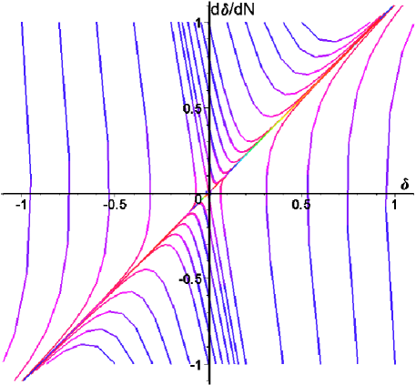
Figure 1: Plot of the solutions of equation (14) for the chaotic model $V(\varphi)=\lambda\varphi^{4}/4$. Each curve corresponds to a different solution starting at $N_{i}=0$ (blue) and running towards $N_{f}=100$ (red).

Note that the value of $n$ does not modify the qualitative behavior of these solutions, while the value of $\lambda$ does not play any rôle at all. Hence, we can conclude that for this kind of models the solution obtained to second order in the horizon-flow functions will typically depart from the lowest orders solutions.

The phase diagrams for the damping and forcing given correspondingly by (24) and (25), or by (26) and (27), are topologically equivalent to that in figure 1. Therefore, it is confirmed the result in the previous section about solutions to Eq. (14) diverging around a saddle-point near the origin, as the generic dynamical pattern for those cases which are interesting from the point of view of inflationary cosmology.

5 Discussion

The rigorous conclusion to be drawn from the results presented in this paper is that solutions of the inverse problem for the inflaton potential obtained using expressions up to second order in the slow-roll approximation will be generically very different from those solutions obtained using lower order expressions.

It may happen that including higher orders helps to get rid of this trouble. However, the order of the expressions used to predict the inflationary spectra is determined by the accuracy of the data from the observations of the CMBR anisotropies and large-scale matter distribution. As it has been pointed out, second order expressions will indeed match the precision of current and near future measurements [9, 5]. In order words, in the expressions for the amplitudes of the inflationary spectra, horizon-flow functions with orders higher than $2$ would not contain any useful information. Therefore, including such orders would be irrelevant for the output of the inverse problem.

Note now that equation (14) has trivial solution $\delta(N)=0$ only for the cases of de Sitter (where $\epsilon_{m}=0$ for $m>0$ ) and power-law inflation [38]. In this last model $a\propto t^{p}$ (with a constant $p\gg 1$), implying $d_{\rm H}\propto\exp(N/p)$, $\epsilon_{1}=1/p$, $\epsilon_{m}=0$ for $m>1$ and $V(\varphi)=\Lambda\exp(B\varphi)$. Here $B$ is a real constant which is zero for a universe dominated by a cosmological constant. Therefore, $\delta(N)$ actually measures the depart from an exponential of the functional form of the output potential. Power-law inflation is the unique model which predicts exact power laws for the amplitudes of both the tensor and scalar spectra [39], i.e., $A(k)=A_{*}k^{n}$, where $k$ is the comoving wavenumber and $n$ is a constant called the spectral index. Moreover, during power-law inflation the scalar index $n_{\rm S}$ is equal to the tensor $n_{\rm T}$, what implies a constant ratio of tensor to scalar amplitudes, $r$. Conversely, in Ref. [30] it was proved that using power-law spectra as input in the inverse problem renders the exponential potential as the unique output. From this point of view, $\delta(N)$ measures the depart of the behavior of the inflationary spectra from a power-law. We can conclude that the essence of the troubles for observing the inflaton potential is the weak signal in the CMBR of scale-dependence of the primordial spectra and the difficulties to extract that information from data using expressions for the inflationary perturbations based on the slow-roll approximation.

As a matter of fact, we were able to clarify here a point which evidences can be traced back in the existing research literature. In 1995, Lidsey et al. [20] showed that the results for the spectra obtained to first order in the slow-roll approximation by Stewart and Lyth [7] could be understood as an expansion about the exact solution for power-law inflation. Two years later, Wang et al. [40] analyzed the implications that finite orders in such an expansion have for precisely predicting the inflationary spectra. Limitations pointed out were linked to the Bessel and horizon-crossing approximations. Martin et al. [41] quantified these limitations by comparing a power-law parametrization for the amplitudes with a more general Taylor series parametrization, and by analyzing the impact of the variation of the pivot scale on the accuracy of predictions. The larger the scale-dependence of the spectra, the bigger is this impact (see also Ref. [27]).

The combination of the Bessel and slow-roll approximations is no longer needed to calculate the primordial spectra, and the power-law parametrization has been extended to included the running of the scalar index. However, the slow-roll condition remains on the basis of the expressions that usually link the Taylor parametrized spectra and the inflationary predictions. There is evidence that the above mentioned limitations still persist. Comparing approximated and numerical predictions for three given models, in Ref. [9] it was noted that increasing the order of the horizon-flow functions beyond the quadratic in every included term of the Taylor parametrization of primordial spectra does not significantly improve the accuracy of the approximations. In fact, adding terms in that parametrization actually seems to be most important for increasing the precision of the predictions. However, the number of terms in the parametrization depends on the capability of the observations to measure a significant departure from scale-invariance in the primordial spectra. As a final evidence, we recall that using first order expressions for $r$ and $n_{\rm S}$, Dodelson et al. were able to discriminate among inflationary models with decreasing and increasing kinetic energy density by distributing them in the $(r,n_{\rm S})$ plane [24]. As it was noted in Ref. [9], including higher order corrections makes impossible to distinguish between these models on the basis of a $r-n_{\rm S}$ plot, unless the running of the spectral index is known or constrained to be very small. The same conclusion was recently made by Kinney and Riotto [27].

Limitations from theoretical and observational sides to account for the scale-dependence of the primordial spectra have been misunderstood as generic predictions of inflation. That this scale-dependence is in the edge of observational capabilities does not means that all the successful inflaton potentials must resemblance an exponential during the inflationary era, but just that we are unable so far to observe the difference. The findings by Hoffman and Turner [42] about power-law inflation as an $\alpha$-attractor (attractor in the future) of the flow in the space of inflationary models were constrained by the order of the expressions in their analysis. As it was shown in Ref. [43], departure from power-law behavior is nullified whenever the leading order is used. To first order, for instance, it remains true that the inflationary dynamics yielding a constant tensor index $n_{\rm T}$ has power-law inflation as an $\alpha$-attractor [30]. Nevertheless, it is also true that the inflationary dynamics characterized by a constant ratio $r$, has power-law inflation as an $\omega$-attractor (attractor in the past or repellor) [31]. Furthermore, in Ref. [32] it was shown how a minimal scale-dependence for $r$ (and information on such a scale-dependence can be drawn from the difference between both spectral indices) allows for models with power-law inflation as a transient regime. Based on these facts, we conjecture here that, if using higher orders in the slow-roll expansion for the analysis of the inflationary flow, power-law inflation still arises as a fixed point, then it will do it like a saddle-point, consistently with the results presented in this paper.

Summarizing, either the slow-roll expansion does not converge or it does so slowly that a large number of terms in this expansion is required to probe the scale dependence of the primordial spectra. Nevertheless, information on this dependence seems to be a necessary ingredient for a robust solution to the inflaton potential inverse problem. This conclusion should encourage further development of the full-numerical method for the resolution of this inverse problem [21], as well as of other analytical methods, for instance, those based on the WKB [11] approximation, on the uniform approximation [12], and on the inverse-scattering theory [25].

References

References

- [1] Bennett C L et al., First year Wilkinson Microwave Anisotropy Probe (WMAP) observations: preliminary maps and basic results, 2003 Astrophys. J. Suppl. 148 1 [astro-ph/0302207]; Spergel D N et al., First year Wilkinson Microwave Anisotropy Probe (WMAP) observations: determination of cosmological parameters, 2003 Astrophys. J. Suppl. 148 175 [astro-ph/0302209].
- [2] Percival W J et al., The 2dF Galaxy Redshift Survey: the power spectrum and the matter content of the universe, 2001 Mon. Not. Roy. Astron. Soc. 327 1297 [astro-ph/0105252]; Tegmark M, Hamilton A J S and Xu Y, The power spectrum of galaxies in the 2dF 100k redshift survey, 2002 Mon. Not. Roy. Astron. Soc. 335 887 [astro-ph/0111575]; Tegmark M et al. [SDSS Collaboration], The 3D power spectrum of galaxies from the SDSS, 2003 [astro-ph/0310725]; J. K. Adelman-McCarthy et al. [SDSS Collaboration], “The Fourth Data Release of the Sloan Digital Sky Survey,” [arXiv:astro-ph/0507711]; Tegmark M et al. [SDSS Collaboration], Cosmological parameters from SDSS and WMAP, 2003 [astro-ph/0310723].
- [3] Mukhanov V F and Chibisov G V, Quantum fluctuation and ‘nonsingular’ universe, 1981 JETP Lett. 33 532 [Pisma Zh. Eksp. Teor. Fiz. 33 549]; Starobinsky A A, Spectrum of relict gravitational radiation and the early state of the universe, 1979 JETP Lett. 30 682 [Pisma Zh. Eksp. Teor. Fiz. 30 719].
- [4] Schwarz D J, Terrero-Escalante C A and Garcia A A, Higher order corrections to primordial spectra from cosmological inflation, 2001 Phys. Lett. B 517 243 [astro-ph/0106020].
- [5] A. Makarov, On the accuracy of slow-roll inflation given current observational constraints, 2005 arXiv:astro-ph/0506326.
- [6] Leach S M, Liddle A R, Martin J and Schwarz D J, Cosmological parameter estimation and the inflationary cosmology, 2002 Phys. Rev. D 66 023515 [astro-ph/0202094].
- [7] Stewart E D and Lyth D H, A more accurate analytic calculation of the spectrum of cosmological perturbations produced during inflation, 1993 Phys. Lett. B 302 171 [gr-qc/9302019].
- [8] I. J. Grivell and A. R. Liddle, Accurate determination of inflationary perturbations, 1996 Phys. Rev. D 54 7191 [arXiv:astro-ph/9607096].
- [9] D. J. Schwarz and C. A. Terrero-Escalante, Primordial fluctuations and cosmological inflation after WMAP 1.0, 2004 JCAP 0408 003 [arXiv:hep-ph/0403129].
- [10] Stewart E D and Gong J O, The density perturbation power spectrum to second-order corrections in the slow-roll expansion, 2001 Phys. Lett. B 510 1 [astro-ph/0101225].
- [11] J. Martin and D. J. Schwarz, WKB approximation for inflationary cosmological perturbations, 2003 Phys. Rev. D 67 083512 [arXiv:astro-ph/0210090]; R. Casadio, F. Finelli, M. Luzzi and G. Venturi, Higher order slow-roll predictions for inflation, 2005 Phys. Lett. B 625 1 [arXiv:gr-qc/0506043]; R. Casadio, F. Finelli, M. Luzzi and G. Venturi, Improved WKB analysis of slow-roll inflation, 2005 arXiv:gr-qc/0510103.
- [12] S. Habib, A. Heinen, K. Heitmann, G. Jungman and C. Molina-Paris, Characterizing inflationary perturbations: The uniform approximation, 2004 Phys. Rev. D 70 083507 [arXiv:astro-ph/0406134]; S. Habib, A. Heinen, K. Heitmann and G. Jungman, Inflationary perturbations and precision cosmology, 2005 Phys. Rev. D 71 043518 [arXiv:astro-ph/0501130].
- [13] J. Choe, J. O. Gong and E. D. Stewart, Second order general slow-roll power spectrum, 2004 JCAP 0407 012 [arXiv:hep-ph/0405155].
- [14] H. M. Hodges and G. R. Blumenthal, Arbitrariness Of Inflationary Fluctuation Spectra, 1990 Phys. Rev. D 42 3329.
- [15] E. J. Copeland, E. W. Kolb, A. R. Liddle and J. E. Lidsey, Reconstructing the inflation potential, in principle and in practice, 1993 Phys. Rev. D 48 2529 [arXiv:hep-ph/9303288].
- [16] G. Mangano, G. Miele and C. Stornaiolo, Inflaton potential reconstruction and generalized equations of state, 1995 Mod. Phys. Lett. A 10 1977 [arXiv:astro-ph/9507117].
- [17] E. W. Mielke and F. E. Schunck, Reconstructing the inflaton potential for an almost flat COBE spectrum, 1995 Phys. Rev. D 52 672 [arXiv:gr-qc/9602029].
- [18] E. Ayon-Beato, A. Garcia, R. Mansilla and C. A. Terrero-Escalante, The Stewart-Lyth inverse problem, Phys. Rev. D 62 103513 [arXiv:astro-ph/0007477].
- [19] E. J. Copeland, E. W. Kolb, A. R. Liddle and J. E. Lidsey, Observing the inflaton potential, 1993 Phys. Rev. Lett. 71 219 [arXiv:hep-ph/9304228].
- [20] J. E. Lidsey, A. R. Liddle, E. W. Kolb, E. J. Copeland, T. Barreiro and M. Abney, Reconstructing the inflaton potential: An overview, 1997 Rev. Mod. Phys. 69 373 [arXiv:astro-ph/9508078].
- [21] I. J. Grivell and A. R. Liddle, Inflaton potential reconstruction without slow-roll, 2000 Phys. Rev. D 61 081301 [arXiv:astro-ph/9906327].
- [22] R. Easther and W. H. Kinney, Monte Carlo reconstruction of the inflationary potential, 2003 Phys. Rev. D 67 043511 [arXiv:astro-ph/0210345].
- [23] E. J. Copeland, I. J. Grivell, E. W. Kolb and A. R. Liddle, On the reliability of inflaton potential reconstruction, 1998 Phys. Rev. D 58 043002 [arXiv:astro-ph/9802209].
- [24] Dodelson S, Kinney W H and Kolb E W, Cosmic microwave background measurements can discriminate among inflation models, 1997 Phys. Rev. D 56 3207 [astro-ph/9702166].
- [25] S. Habib, K. Heitmann and G. Jungman, Inverse-Scattering Theory and the Density Perturbations from Inflation, 2005 Phys. Rev. Lett. 94 061303 [arXiv:astro-ph/0409599].
- [26] K. Kadota, S. Dodelson, W. Hu and E. D. Stewart, Precision of inflaton potential reconstruction from CMB using the general slow-roll approximation, 2005 Phys. Rev. D 72 023510.
- [27] W. H. Kinney and A. Riotto, Theoretical uncertainties in inflationary predictions, 2005 arXiv:astro-ph/0511127.
- [28] C. A. Terrero-Escalante, Cosmic acceleration, scalar fields and observations, 2004 Lect. Notes Phys. 646 109 [arXiv:astro-ph/0404591].
- [29] J. E. Ruhl et al. The South Pole Telescope, 2004 [arXiv:astro-ph/0411122]; PLANCK Mission: http://www.rssd.esa.int/SA/PLANCK/include/report/redbook/redbook-science.htm; The Big Bang Observer: http://universe.nasa.gov/program/bbo.html.
- [30] C. A. Terrero-Escalante, E. Ayon-Beato and A. A. Garcia, Inflationary scenarios with scale-invariant spectral tensorial index, 2001 Phys. Rev. D 64 023503 [arXiv:astro-ph/0101522].
- [31] C. A. Terrero-Escalante, J. E. Lidsey and A. A. Garcia, Inflation with a constant ratio of scalar and tensor perturbation amplitudes, 2002 Phys. Rev. D 65 083509 [arXiv:astro-ph/0111128].
- [32] C. A. Terrero-Escalante, Tensor to scalar ratio of perturbation amplitudes and inflaton dynamics, 2003 Phys. Lett. B 563 15 [arXiv:astro-ph/0209162].
- [33] V. I. Arnold, Ordinary differential equations. Nauka, Moscow, 1984 (in Russian).
- [34] C. A. Terrero-Escalante, On bounded solutions for second order linear differential equations with negative stiffness, 2005, arXiv:math.CA/0511222.
- [35] Linde A D, Eternally Existing Selfreproducing Chaotic Inflationary Universe, 1986 Phys. Lett. B 175 395.
- [36] Binétruy P and Gaillard M K, Candidates for the Inflaton Field in Superstring Models, 1986 Phys. Rev. D 34 3069.
- [37] Linde A D, Axions in inflationary cosmology, 1991 Phys. Lett. B 259 38.
- [38] Lucchin F and Matarrese S, Power Law Inflation, 1985 Phys. Rev. D 32 1316.
- [39] L. F. Abbott and M. B. Wise, Constraints On Generalized Inflationary Cosmologies, 1984 Nucl. Phys. B 244 541.
- [40] Wang L M, Mukhanov V F and Steinhardt P J, On the problem of predicting inflationary perturbations, 1997 Phys. Lett. B 414 18 [astro-ph/9709032].
- [41] Martin J and Schwarz D J, The precision of slow-roll predictions for the CMBR anisotropies, 2000 Phys. Rev. D 62 103520 [arXiv:astro-ph/9911225]; J. Martin, A. Riazuelo and D. J. Schwarz, Slow-roll inflation and CMB anisotropy data, 2000 Astrophys. J. 543 L99 [arXiv:astro-ph/0006392].
- [42] M. B. Hoffman and M. S. Turner, Phys. Rev. D 64 (2001) 023506 [arXiv:astro-ph/0006321].
- [43] Terrero-Escalante C A, 2003 Is power law inflation really attractive?, Rev. Mex. Fis. 49S2 118 [arXiv:astro-ph/0204066].