Towards testing interacting cosmology by distant type Ia supernovae

Abstract

We investigate the possibility of testing cosmological models with interaction between matter and energy sector. We assume the standard FRW model while the so called energy conservation condition is interpreted locally in terms of energy transfer. We analyze two forms of dark energy sectors: the cosmological constant and phantom field. We find a simple exact solution of the models in which energy transfer is described by a Cardassian like term in the relation of $H^{2}(z)$, where $H$ is Hubble’s function and $z$ is redshift. The considered models have two additional parameters $(\Omega_{\text{int}},n)$ (apart the parameters of the $\Lambda$CDM model) which can be tested using SNIa data. In the estimation of the model parameters Riess et al.’s sample is used. We also confront the quality of statistical fits for both the $\Lambda$CDM model and the interacting models with the help of the Akaike and Bayesian informative criteria. Our conclusion from standard best fit method is that the interacting models explains the acceleration of the Universe better but they give rise to a universe with high matter density. However, using the tools of information criteria we find that the two new parameters play an insufficient role in improving the fit to SNIa data and the standard $\Lambda$CDM model is still preferred. We conclude that high precision detection of high redshift supernovae could supply data capable of justifying adoption of new parameters.

I Introduction

The main aim of the paper is to use the distant type Ia supernovae (SNIa) compiled by Riess et al. Riess et al. (2004) to analyze the interacting cosmology (or cosmology with energy transfer) which was recently proposed by Zimdahl and Pavon Zimdahl and Pavon (2004) and Zhang Zhang (2005) as a way to explain the coincidence conundrum of the ratio of dark matter to dark energy density at present. We show that allowed intervals for two independent parameters which characterize interacting cosmology give rise to high matter density, which can hardly be reconciled with the current value obtained from cluster baryon fraction measurements.

The major development of modern cosmology, which mainly concentrates on observational cosmology, seems to be a discovery of the acceleration of the universe through distant SNIa. In principal there are three different theoretical types of explanation of acceleration. In the first group the existence of matter of unknown forms violating the strong energy condition is postulated (dark energy). In the second group instead of dark energy some modification of the FRW equation is proposed. Between these two propositions lies an idea of interacting cosmology in which the source of acceleration lies in interaction between dark energy and dark matter sector.

The starting point of any investigations in observational cosmology is the naive FRW model (the $\Lambda$CDM model) in which matter and dark energy sectors do not interact with each other. The next step in making this model more realistic is to include the interaction between dark matter and dark energy. We start with the FRW standard cosmological equations: the Raychaundhuri equation and conservation condition. They assume the following forms respectively

$$\frac{\ddot{a}}{a} =-\frac{1}{6}(\rho+3p)$$ (1)

$$\dot{\rho} =-3H(\rho+p),$$ (2)

where $a$ is the scale factor, $\rho$ and $p$ are energy density and pressure of perfect fluid, a source of gravity; $H=\dot{a}/a$ is the Hubble function, and a dot means differentiation with respect to the cosmological time $t$. It would be convenient to rewrite relation (2) for mixture of dust matter and dark energy

$$\frac{1}{a^{3}}\frac{d}{dt}\left(\rho_{\text{m}}a^{3}\right)+\frac{1}{a^{3(1+w_{X})}}\frac{d}{dt}\left(\rho_{X}a^{3(1+w_{X})}\right)=0,$$ (3)

where the total pressure and energy density are

$$p =0+w_{X}\rho_{X},\quad w_{X}=p_{X}/\rho_{X}=\text{const}$$ (4)

$$\rho =\rho_{\text{m}}+\rho_{X}$$ (5)

The standard postulate of the $\Lambda$CDM model is that both terms in eq. (3) are equal to zero, or that the matter components evolve independently. We, however, assume the existence of interaction introducing a non-vanishing function $\gamma(t)$ such that eq. (3) is still satisfied locally

$$\frac{1}{a^{3}}\frac{d}{dt}\left(\rho_{\text{m}}a^{3}\right) \equiv\gamma(t)$$ (6)

$$\frac{1}{a^{3(1+w_{X})}}\frac{d}{dt}\left(\rho_{X}a^{3(1+w_{X})}\right) \equiv-\gamma(t)$$ (7)

Note that $\gamma(t)$ in (6)-(7) has the interpretation of the rate of change of energy in the unit comoving volume.

We only assume the existence of the energy transfer without specifying its physical mechanism, then test it by astronomical observations. The idea of such decomposition of the conservation condition (6)-(7) is not new Zimdahl et al. (2001). The interacting quintessence models with pressureless cold dark matter fluid can give rise to the scale factor relation $\rho_{X}/\rho_{\text{m}}=a^{\xi}$ Hoffman (2003); Pavon et al. (2004), where $\xi$ is a constant parameter. This relation was also tested by CMB WMAP observations and statistically investigated in the context of SNIa observations Zimdahl and Pavon (2003) but with the help of a different exact solution. In the paper of one of us Szydlowski (2005), this idea was investigated independently without any physical assumption or about the form of such an interaction or an exact solution. Under such general assumptions, that the FRW dynamics is valid, the existence of energy transfer to the dark energy sector from the dark matter section is favored by SNIa data. However, if we apply the prior $\Omega_{\text{m},0}=0.3$ as claimed by independent galactic observations, then the transfer between dark matter and phantom sector is required. The proposition of different physical mechanism of energy exchange from dark energy to dark matter sectors was proposed by many authors Ziaeepour (2004); Svetlichny (2005); Zhang and Zhu (2005).

We consider models where the rate of energy transfer is proportional to the rate of change of the scale factor $\gamma(t)=f(a)H$.

While the standard statistical methods of maximum likelihood used for estimation of the model parameters favor the energy transfer between dark matter and phantom dark energy sector, we demonstrate by the means of the Akaike and Bayesian information criteria that the $\Lambda$CDM model with interaction is selected.

II The FRW model with interaction

We assume for simplicity of presentation without loss of generality a simple flat model for which we have the Friedmann first integral in the form

$$3\dot{a}^{2}=a^{2}(\rho_{\text{m}}+\rho_{X})$$ (8)

In the case of non-flat models relation (8) is of the form

$$3\dot{a}^{2}=a^{2}(\rho_{\text{m}}+\rho_{X})-3k$$ (9)

We add to equation (8) the generalized adiabatic condition

$$\frac{d}{dt}\rho_{\text{m}} =-3H\rho_{\text{m}}+\gamma(t),$$ (10)

$$\frac{d}{dt}\rho_{X} =-3(1+w_{X})H\rho_{X}-\gamma(t),$$ (11)

$$\frac{d}{dt}H =-H^{2}-\frac{1}{6}(\rho_{\text{m}}+\rho_{X})$$ (12)

from which we obtain

$$\frac{d(\ln\rho_{\text{m}})}{d(\ln a)} \equiv I_{a}(\rho_{\text{m}})=-3+\frac{\gamma}{H\rho_{\text{m}}}$$ (13)

$$\frac{d(\ln\rho_{x})}{d(\ln a)} \equiv I_{a}(\rho_{X})=-3(1+w_{X})-\frac{\gamma}{H\rho_{X}}$$ (14)

$$\frac{d(\ln(\rho_{\text{m}}/\rho_{X})}{d(\ln a)} =3w_{X}+\frac{1}{H}\left(\frac{1}{\rho_{\text{m}}}+\frac{1}{\rho_{X}}\right)$$ (15)

where $I_{a}(\rho_{\text{m}})$ and $I_{a}(\rho_{X})$ have the interpretation of elasticity (logarithmic slope) of the energy densities with respect to the scale factor. If energy transfer vanishes then the corresponding elasticity function becomes constant. From (13)-(14) we can simply derive the relation

$$I_{a}\left(\frac{\rho_{\text{m}}}{\rho_{X}}\right)=\frac{d\ln\left(\frac{\rho_{\text{m}}}{\rho_{X}}\right)}{d(\ln a)}=3w_{X}+\frac{3\gamma H}{\rho_{\text{m}}\rho_{X}}$$ (16)

Therefore scaling solutions $\rho_{\text{m}}/\rho_{X}\propto a^{\xi}$ can only be realized if a very special form of parameterization $\gamma(t)$ is assumed Zimdahl et al. (2001); Pavon et al. (2004); Zimdahl and Pavon (2003), namely

$$\gamma(t)=\gamma_{0}H\frac{1}{\frac{1}{\rho_{\text{m}}}+\frac{1}{\rho_{X}}}=\gamma_{0}\bar{\rho}\,^{-1}H,$$ (17)

where $\bar{\rho}$ is the harmonic average of $\rho_{\text{m}}$ and $\rho_{X}$. It is interesting to discuss the existence of scaling solutions for other parameterizations of $\gamma(t)$. For this purpose the methods of dynamical systems can be useful because they offer possibility of investigating all admissible evolutional paths for all initial conditions. Let us consider the following distinguished case.

Let $\gamma(t)=\gamma_{0}f(a)H$ and $f(a)=a^{m}$. In this case one can find exact solutions determining energy densities

$$\rho_{\text{m}} =\frac{\gamma_{0}}{m+5}a^{m+2}+\frac{A_{\text{m},0}}{a^{3}}$$ (18)

$$\rho_{X} =-\frac{\gamma_{0}}{m+5+3w_{X}}a^{m+2}+\frac{A_{\text{m},0}}{a^{3(1+w_{X})}}$$ (19)

where in the special cases of $m=-5$ and $m=-5-3w_{X}$ instead of a power law function a logarithmic function appears; $A_{\text{m},0}$ and $A_{X,0}$ are constants. Note that the contribution to the total energy arising from interaction is of the type $a^{-m-2}$, therefore it can be modelled by some additional fictitious fluid satisfying the equation of state $p_{\text{int}}=-(m+5)\rho_{\text{int}}/3$.

In terms of redshift $z$ we obtain the basic relation

$$H^{2}=H_{0}^{2}\left(\Omega_{\text{int}}(1+z)^{-m-2}+\Omega_{\text{m},0}(1+z)^{3}+\Omega_{X,0}(1+z)^{3(1+w_{X})}+\Omega_{k,0}(1+z)^{2}\right),$$ (20)

where

$$\Omega_{int,0}=\frac{3w_{X}}{(m+5)(m+5+3w_{X})}\gamma_{0},$$ (21)

and the index zero means that quantities are evaluated at the present moment. The relation will be useful in the next section where both $\Omega_{\text{int}}$ and $m$ parameters will be fitted to SNIa data.

For formulation the corresponding dynamical system it would be useful to represent this case in the form of the Hamiltonian dynamical system. For this case it is sufficient to construct the potential function

$$V=-\frac{\rho_{\text{eff}}a^{2}}{6}$$ (22)

which build the Hamiltonian

$$\mathcal{H}=\frac{\dot{a}^{2}}{2}+V(a).$$ (23)

We find that the Hamiltonian system is determined on the zero level $\mathcal{H}=0$ and the potential function in terms of the scale factor expressed in units of its present value $a_{0}$, $x=\frac{a}{a_{0}}$, is

$$V(x)=-\frac{1}{2}\Omega_{\text{m},0}x^{-1}-\frac{1}{2}\Omega_{w_{X},0}x^{-3(1+w_{X})+2}-\frac{1}{2}\Omega_{\text{int}}x^{-m}-\frac{1}{2}\Omega_{k,0}.$$ (24)

The Hamiltonian constraint gives rise to the relation $\sum_{i}\Omega_{i,0}=1$. The corresponding dynamical system is of the form

$$\dot{x} =y$$ (25)

$$\dot{y} =-\frac{\partial V}{\partial x}$$ (26)

and $\mathcal{H}=0$ plays the role of first integral of (25)-(26). Advantages of representing dynamics in the form (25)-(26) is that the critical points as well as their character can be determined from the geometry of the potential function only. Only the static critical points, admissible in the finite domain, $y_{0}=0|_{x_{0}}$, $\frac{\partial V}{\partial x}=0$ are saddles or centers. The eigenvalues of the linearization matrix are

$$\lambda_{1,2}=\pm\sqrt{-\left(\frac{\partial^{2}V}{\partial x^{2}}\right)_{x_{0}}}$$ (27)

The phase portraits on the phase plane $(x,\dot{x})$ are shown in Fig. 1 ($w=-1$, “decaying” vacuum cosmology) and in Fig. 2 ($w=-\frac{4}{3}$, phantom fields). We can observe the existence of a single static critical point located on the $x$-axis and the topological equivalence of these phase portraits in the finite domain. In both cases we have static critical points situated on the $x$-axis. They are of saddle type because the potential function is upper convex. We have also the critical points at infinity which represent stable nodes. They represent the de Sitter model in Fig. 1 and the big rip singularity in Fig. 2. The big rip singularity is generic future of the model violating weak energy condition at which the scale factor is infinite at some finite time Dabrowski et al. (2003).

Figure 1: The phase portrait for the $\Lambda$ interacting cosmological model. The trajectories of flat model separate the domains of closed and open models

Figure 2: The phase portrait for the phantom interacting cosmological model.

In connection with the present value of the density parameters $\Omega_{\text{m},0}$ and $\Omega_{X,0}$ there arises the coincidence problem. Why are the energy densities of dark energy and dark matter of the same order amplitude at the present epoch? Dalal et al. (2001); Sahni (2002); Gorini et al. (2004); Huey and Wandelt (2004). In this context we can use some interesting idea formulated by Amendola and Tocchini-Valentini Amendola and Tocchini-Valentini (2001) who argue that the present state of the accelerating universe is described by the global attractor in the phase space. It seems to be reasonable to treat the evolution of the interacting universe model with tools of dynamical system methods. From the physical point of view the critical points represent asymptotic state of the system reached in infinite time. Let us assume that $\gamma(t)$ is proportional to the Hubble parameter, i.e. $\gamma(t)\propto\bar{\gamma}(\rho_{\text{m}},\rho_{X})H$ Zimdahl et al. (2001); Pavon et al. (2004); Zimdahl and Pavon (2003) then after the reparametrization of the time variable $t\to\tau\colon Hdt=d\tau$, we obtain the two-dimensional closed dynamical system in the form

$$\frac{d\rho_{\text{m}}}{d\tau} =-3\rho_{\text{m}}+\bar{\gamma}(\rho_{\text{m}},\rho_{X})$$ (28)

$$\frac{d\rho_{X}}{d\tau} =-3(1+w)-\bar{\gamma}(\rho_{\text{m}},\rho_{X}).$$ (29)

System (28)-(29) has a critical point at which

$$\Omega_{X,0}/\Omega_{\text{m},0}=-(1+w)^{-1}.$$

In the case of phantom ($w=-4/3$) we obtain $\Omega_{X,0}/\Omega_{\text{m},0}=3$. This critical point is stable if a trace of a linearization matrix is negative at this point, i.e., $\partial(-\bar{\gamma})/\partial\rho_{\text{m}}>\partial(-\bar{\gamma})/\partial\rho_{X}-2$. If $\bar{\gamma}\propto-\rho_{\text{m}}\rho_{X}$ it means that $\Omega_{X,0}>\Omega_{\text{m},0}$.

In Fig. 3 we observe that the most probable values of $n=-m-2$ and $\Omega_{\text{int},0}$ are close to zero. In Fig. 4 there is two disjoint region which are preferred, while values of $n$ and $\Omega_{\text{int},0}$ close to zero are excluded at the 95% confidence level.

Figure 3: Confidence levels on the plane $(\Omega_{\text{int}},n)$ for the interaction between matter and the $\Lambda$ vacuum energy sectors; the prior on $\Omega_{\text{m},0}=0.3$ is assumed.

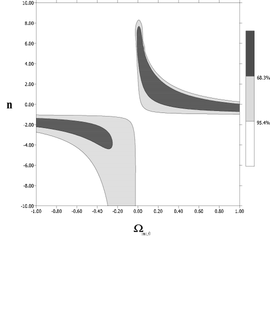
Figure 4: Confidence levels on the plane $(\Omega_{\text{int}},n)$ for the interaction between matter and the phantom sectors; the prior on $\Omega_{\text{m},0}=0.3$ is assumed.

For deeper statistical analysis it is useful to consider the probability distribution function (PDF) over model parameters. On Fig. 5, 6, 7 the one-dimensional PDF are demonstrated for $\Omega_{\text{int},0}$, $n$, $\Omega_{\Lambda,0}$.

Figure 5: The PDF for $(\Omega_{\text{int},0})$ when matter interacts with the “decaying” vacuum (left) and matter interacts with phantom field (right); the prior on $\Omega_{\text{m},0}=0.3$ is assumed.

Figure 6: The PDF for $n$ when matter interacts with the “decaying” vacuum (left) and matter interacts with phantom field (right); the prior on $\Omega_{\text{m},0}=0.3$ is assumed.

Figure 7: The PDF for $(\Omega_{\Lambda,0})$ when matter interacts with the “decaying” vacuum (left) and matter interacts with phantom field (right); the prior on $\Omega_{\text{m},0}=0.3$ is assumed

III Discussion of results

We use the maximum likelihood method to estimate two basic parameters of the cosmology with interaction. The priors we assume for numerical computations are: $-10<n<10$, $-1<\Omega_{\text{int}}<1$, $0<\Omega_{\text{m},0}<1$ (or fixed at $0.3$), and the other density parameter determined from $\sum_{i}\Omega_{i}=1$. From this statistical analysis we obtained that with assumed $\Omega_{\text{m},0}=0.3$ the interaction between “decaying” $\Lambda$ and matter sectors is negligible while the interaction between phantom and matter sector is required (see Table 1). The analogous analysis without any priors contains (see Table 2).

To select between these models we use the Akaike and Bayesian information criteria (AIC and BIC) Liddle (2004); Szydlowski et al. (2005); Godlowski and Szydlowski (2005). These criteria were proposed to answer the question whether or not new parameters are relevant in the estimation. In the generic case introducing new parameters allows to improve the fit to the dataset, however information criteria try to measure whether the improvement in fit is large enough to consider it statistically significant.

When we consider the interacting cosmological model we add two new parameters describing the interaction to the base $\Lambda$CDM model. Using the AIC and BIC we compare the fits of these two models to the most recent sample of SNIa (see Table 3).

To improve the statistical analysis and obtain more precise physical results it is necessary to extend the sample to higher redshifts $z>1.5$. Given two mechanisms of interaction between dark energy and dark matter sectors, we found that the $\Lambda$CDM model is favored over the “decaying” $\Lambda$ interacting model ($\Lambda$INT) but it is disfavored over phantom interacting model (PhINT) for both criteria. The same result is obtained independently of using the prior on $\Omega_{\text{m},0}$.

It is an interesting question whether it is possible to determine the direction of energy transfer from SNIa data. To this aim we calculate the probability that $\gamma_{0}$ is greater than zero $P(\gamma_{0}>0)$ as well as find the most probable values of the parameters. We have

$$P(\gamma_{0}>0) =35\% \Lambda$$ for Int models (30)

$$P(\gamma_{0}>0) =82.81\% \text{for PhInt models},$$

under the constraint $\Omega_{\text{m},0}=0.3$. Therefore, with the confidence level of 95% we can’t exclude any direction of energy transfer. Because this result is inconclusive, we check the sign of $\gamma_{0}$ for the most probable values of the parameters. In both cases, we obtain (independently of assuming the fixed prior for $\Omega_{\text{m},0}$) that $\gamma_{0}<0$. Let us also note that in the case of the PhIntCDM model the values $\Omega_{\text{int},0}=0$ and $n=0$ are excluded with the confidence level of 95%.

Both the maximum likelihood method and the best fit method are used principally to estimate the values of parameters. Additionally the best fit method allows to choose the best model when a few models are to consider. However there is a serious shortcoming of the best fit method because models with greater number of parameters are generally preferred. To overcome this drawback and push the statistical analysis one step further we employ the model selection criteria. It can be seen as the second stage of statistical analysis after the estimation. Both of the used information criteria, the AIC and BIC, put some penalty on adding additional parameters assigning a threshold which should be exceeded to consider a model with a greater number of parameters to be a better fit.

Table 1: Results of the statistical analysis of the model obtained both for Riess et al. samples from the best fit with minimum $\chi^{2}$ (denoted with BF) and from the likelihood method (denoted with L). The same analysis was repeated with fixed $\Omega_{\text{m},0}=0.3$ (denoted F).

sample	$\Omega_{\text{m},0}$	$\Omega_{\text{int},0}$	$n=-m-2$	$\Omega_{\Lambda,0}$	$\mathcal{M}$	$\chi^{2}$	method
$\Lambda$CDM	0.31	—	—	0.69	15.955	175.9	BF
	0.44	—	—	0.69	15.955	—	L
	F 0.30	—	—	F0.70	15.955	175.9	BF
	F 0.30	—	—	F0.70	15.955	—	L
$\Lambda$INT	0.43	0.28	-10.00	0.29	15.905	172.1	BF
	0.44	0.34	-2.70	0.20	15.935	—	L
	F 0.30	0.07	-10.00	0.63	15.925	175.2	BF
	F 0.30	0.00	0.00	0.70	15.945	—	L
PhINT	0.46	0.25	-10.00	0.29	15.905	172.2	BF
	0.44	0.26	-2.60	0.62	15.935	—	L
	F 0.30	0.03	5.10	0.67	15.935	173.5	BF
	F 0.30	0.03	0.00	0.67	15.945	—	L

Table 2: Model parameter values obtained from the minimization procedure carried out with the Riess et al. sample.

sample	$\Omega_{\text{m},0}$	$\Omega_{\text{int},0}$	$\Omega_{\Lambda,0}$	$n=-m-2$
$\Lambda$CDM	$0.31^{+0.04}_{-0.04}$	—	$0.69^{+0.04}_{-0.04}$	—
	$0.30$	—	$0.70$	—
$\Lambda$INT	$0.44^{+0.11}_{-0.11}$	$0.34^{+0.39}_{-0.33}$	$0.20^{+0.55}_{-0.47}$	$-2.70^{+1.80}_{-5.70}$
	$0.30$	$0.00^{+0.26}_{-0.17}$	$0.70^{+0.17}_{-0.26}$	$0.00^{+1.50}_{-4.80}$
PhINT	$0.44^{+0.10}_{-0.09}$	$0.26^{+0.50}_{-0.46}$	$0.62^{+0.24}_{-0.76}$	$-2.60^{+5.00}_{-3.10}$
	$0.30$	$0.03^{+0.43}_{-0.03}$	$0.67^{+0.03}_{-0.43}$	$0.00^{+1.50}_{-1.50}$

Table 3: The values of AIC and BIC for distinguished models both for $\Omega_{\text{m},0}$ fitted and for $\Omega_{\text{m},0}=0.3$.

case	AIC (fitted $\Omega_{\text{m},0}$)	AIC ($\Omega_{\text{m},0}=0.3$)	BIC (fitted $\Omega_{\text{m},0}$)	BIC ($\Omega_{\text{m},0}=0.3$)
$\Lambda$CDM	179.9	177.9	186.0	181.0
$\Lambda$INT	180.1	181.2	192.3	190.4
PhINT	180.2	179.5	192.4	188.7