Apparent Hubble acceleration from
large-scale electroweak domain structure

Abstract

The observed luminosity deficit of Type Ia supernovae (SNe Ia) at high redshift $z$ can be explained by partial conversion to weak vector bosons of photons crossing large-scale electroweak domain boundaries, making Hubble acceleration only apparent and eliminating the need for a cosmological constant $\Lambda>0$.

I Introduction

After the initial surprise caused by the announcement of a luminosity deficit from high redshift $z$ Type Ia supernovae (SNe Ia) riess1998 perlmutter1998 perlmutter1999 , the consensus quickly emerged that we are witnessing an accelerating Hubble expansion, implying a cosmological constant $\Lambda>0$. This has forced a profound change in our view of the large scale structure and composition of the universe, leading us from a preferred model with negative curvature and density parameter $\Omega\approx 0.3$ dominated by (mostly dark) matter to a flat geometry with $\Omega\approx 1$ dominated by the dark energy term $\Omega_{\Lambda}\approx 0.7$ ($\Lambda$CDM). Most importantly from the point of view of fundamental physics, it has also left us with the massive embarrassment of a finite $\Lambda$ 120 orders of magnitude below the Planck scale, where it’s customarily argued on dimensional grounds that the zero point energy of quantum fields coupled to gravity should show up, absent some fundamental principle forcing it to vanish exactly.

These far-reaching implications have motivated many studies of alternative explanations for the dimming of high-$z$ SNe Ia, from variations in intrinsic luminosity (chemical abundances, stellar populations) through modified light propagation (gravitational lensing, gray dust) to systematic observational errors (selection bias) filippenko2003 riess2004 . But to date, all suggested mechanisms have proved incapable of producing effects of the needed size, -0.25 magnitudes at $z\sim 0.5$ (where the luminosity deficit has its greatest leverage on $\Lambda$), i.e. a ratio between observed luminosity $\ell$ and expected luminosity $\ell_{E}$

$$\ell/\ell_{E}\approx 100^{-0.25/5}\approx 0.79$$ (1)

The case for dark energy rests squarely on this number. In spite of common claims to the contrary, dimming of SNe Ia (and now of gamma ray bursts schaefer2006 ) remains the only direct evidence of accelerated expansion blanchard2003 . Even disregarding the possibility of significant systematic errors in distance measures bonanos2006 wang2006 , the oft-quoted consistency of $\Lambda$CDM with other observations is only a necessary condition for its validity, not a sufficient one. The true power of this condition is its ability to falsify the framework: find an explanation for one data set leaving insufficient room for accelerated expansion to fit the others and the entire framework is invalidated.

The main objective of this paper is to show how the standard electroweak and big bang models can lead to the observed $\ell/\ell_{E}$ without any Hubble acceleration actually taking place, and how they are in fact constrained by observation to do so in a way which leaves little room for $\Lambda>0$.

II Photon transformations

In the standard SU(2)$\times$U(1) model of electroweak interactions glashow1961 weinberg1967 salam1968 , the U(1) gauge field $B_{\mu}(x)$ and the three SU(2) gauge fields $W^{j}_{\mu}(x)$ are collected in the matrix (the field-dependent part of the covariant derivative)

$${\bm{M}}_{\mu}(x)\equiv\left[\begin{array}[]{lr}g^{\prime}B_{\mu}(x)+gW^{3}_{\mu}(x)&gW^{1}_{\mu}(x)-igW^{2}_{\mu}(x)\\ gW^{1}_{\mu}(x)+igW^{2}_{\mu}(x)&g^{\prime}B_{\mu}(x)-gW^{3}_{\mu}(x)\end{array}\right]$$ (4)

($g$ = SU(2) coupling constant; $g^{\prime}$ = U(1) coupling constant) acting on weak isospin doublets. Given an arbitrary ${\bm{M}}_{\mu}(x)$, we can decompose it into individual gauge fields using

$$B_{\mu}(x) = \frac{1}{2g^{\prime}}{\rm Tr}\left[\tau_{0}\thinspace{\bm{M}}_{\mu}(x)\right]$$ (5)

$$W^{1}_{\mu}(x) = \frac{1}{2g}{\rm Tr}\left[\tau_{1}\thinspace{\bm{M}}_{\mu}(x)\right]$$ (6)

$$W^{2}_{\mu}(x) = \frac{i}{2g}{\rm Tr}\left[\tau_{2}\thinspace{\bm{M}}_{\mu}(x)\right]$$ (7)

$$W^{3}_{\mu}(x) = \frac{1}{2g}{\rm Tr}\left[\tau_{3}\thinspace{\bm{M}}_{\mu}(x)\right]$$ (8)

where all traces are understood to be over weak isospin space only, $\tau_{0}\equiv{\bm{1}}_{2}$ and $\tau_{1}$, $\tau_{2}$, $\tau_{3}$ are the Pauli matrices

$$\tau_{1}\equiv\left[\begin{array}[]{lr}0&1\\ 1&0\end{array}\right]\quad\tau_{2}\equiv\left[\begin{array}[]{lr}0&-i\\ i&0\end{array}\right]\quad\tau_{3}\equiv\left[\begin{array}[]{lr}1&0\\ 0&-1\end{array}\right]$$ (15)

The photon $A_{\mu}(x)$ and the neutral weak vector boson $Z^{0}_{\mu}(x)$ are defined as the linear combinations

$$\left[\begin{array}[]{c}Z^{0}_{\mu}(x)\\ A_{\mu}(x)\end{array}\right]\equiv\left[\begin{array}[]{lr}\cos(\theta_{W})&-\sin(\theta_{W})\\ \sin(\theta_{W})&\cos(\theta_{W})\end{array}\right]\left[\begin{array}[]{c}W_{\mu}^{3}(x)\\ B_{\mu}(x)\end{array}\right]$$ (22)

where $\theta_{W}$ is the Weinberg (weak mixing) angle,

$$g\sin(\theta_{W})=g^{\prime}\cos(\theta_{W})=e>0$$ (23)

($e$ = electric charge of the proton). Combining (5), (8) and (22), we can therefore write

$$A_{\mu}(x) = \frac{\sin(\theta_{W})}{2g}\thinspace{\rm Tr}\left[\tau_{3}\thinspace{\bm{M}}_{\mu}(x)\right]$$ (24)

$$+ \frac{\cos(\theta_{W})}{2g^{\prime}}\thinspace{\rm Tr}\left[\tau_{0}\thinspace{\bm{M}}_{\mu}(x)\right]$$

Setting $Z^{0}_{\mu}(x)=W^{1}_{\mu}(x)=W^{2}_{\mu}(x)=0$ and $A_{\mu}(x)=1$, inverting (22) and plugging the results into (4) yields ${\bm{M}}_{\mu}(x)$ for a normalized pure photon state:

$${\bm{M}}^{A}_{\mu}=\left[\begin{array}[]{lr}2e&0\\ 0&0\end{array}\right]$$ (27)

(completely delocalized and therefore monochromatic; an envelope can be imposed without consequence for the present argument). Now consider the effect on ${\bm{M}}_{\mu}(x)$ of a global SU(2)$\times$U(1) transformation

$${\bm{U}}\equiv\exp\left({\frac{i}{2}\thinspace\omega_{0}\tau_{0}}+{\frac{i}{2}\thinspace\omega_{j}\tau_{j}}\right)$$ (28)

with U(1) parameter $\omega_{0}$ and SU(2) parameters ${\bm{\omega}}\equiv(\omega_{1},\omega_{2},\omega_{3})$:

$${\bm{M}}_{\mu}(x)\rightarrow{\bm{M}}^{\prime}_{\mu}(x)={\bm{U}}{\bm{M}}_{\mu}(x){\bm{U}}^{\dagger}$$ (29)

Substituting this into (24) and using the cyclic property of the trace,

$$A_{\mu}(x)\rightarrow A^{\prime}_{\mu}(x) = \frac{\sin(\theta_{W})}{2g}\thinspace{\rm Tr}\left[{\bm{U}}^{\dagger}\thinspace\tau_{3}\thinspace{\bm{U}}{\bm{M}}_{\mu}(x)\right]$$ (30)

$$+ \frac{\cos(\theta_{W})}{2g^{\prime}}\thinspace{\rm Tr}\left[{\bm{M}}_{\mu}(x)\right]$$

U(1) transformations associated with $\omega_{0}\tau_{0}$ drop out. Specializing to the pure photon state ${\bm{M}}^{A}_{\mu}$ of (27), introducing the shorthand

$$\omega_{\bot}^{2}\equiv{\omega_{1}^{2}+\omega_{2}^{2}}$$ (31)

$$\omega\equiv\sqrt{\omega_{\bot}^{2}+\omega^{2}_{3}}$$ (32)

and doing the traces, (30) reduces to

$$A_{\mu} \rightarrow A^{\prime}_{\mu}=\ell({\bm{\omega}})A_{\mu}$$ (33)

with

$$\ell({\bm{\omega}})\equiv\sin^{2}(\theta_{W})\frac{\omega_{\bot}^{2}\cos(\omega)+\omega_{3}^{2}}{\omega^{2}}+\cos^{2}(\theta_{W})$$ (34)

(see Fig. 1, 2). Together with (33), equation (34) describes the effect of a global transformation with SU(2) parameters ${\bm{\omega}}$ (and arbitrary U(1) parameter $\omega_{0}$) on a pure photon state. On its own, since $A_{\mu}(x)$ is proportional to the photon number operator, it gives us the fraction of photons surviving the transformation (the rest having turned into $Z^{0}$s and linear combinations of $W^{1}$s and $W^{2}$s, i.e. $W^{\pm}$s). The full import of this residual luminosity $\ell({\bm{\omega}})$ will become evident in Section VII.

Figure 1: Residual luminosity $\ell({\bm{\omega}})$ for $\omega_{\bot}\in[0,\sqrt{32}\pi]$, $\omega_{3}\in[0,4\pi]$ (contour plot).

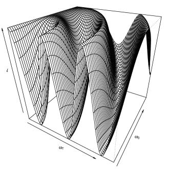
Figure 2: Residual luminosity $\ell({\bm{\omega}})$ for $\omega_{\bot}\in[0,\sqrt{32}\pi]$, $\omega_{3}\in[0,4\pi]$ (perspective plot).

III Electroweak phase transition

In order to give the standard model fields (inertial) mass without explicitly breaking the gauge symmetry of the Lagrangian (needed for renormalizability thooft1971a thooft1971b ), the weak isospin doublet

$$\Phi(x)=\begin{bmatrix}\phi^{+}(x)\\ \phi^{0}(x)\end{bmatrix}$$ (35)

is introduced, where $\phi^{+}(x)$ and $\phi^{0}(x)$ are complex Lorentz scalars transforming under SU(2)$\times$U(1) according to

$$\Phi(x)\rightarrow\Phi^{\prime}(x)={\bm{U}}\Phi(x)$$ (36)

with the ${\bm{U}}$ of (28). Augmenting the Lagrangian with a potential term featuring a manifold of degenerate ground states for $\Phi(x)\neq 0$ (all connected by ${\bm{U}}$) turns $\Phi(x)$ into a Higgs field higgs1964 higgs1966 which breaks the symmetry dynamically by picking a non-zero VEV (vacuum expectation value) $\langle\Phi\rangle$ in a specific ground state. The asymmetric VEV splits the interaction terms between $\Phi(x)$ and the other fields into effective mass terms and new interaction terms involving $\Phi(x)$ excitations above the selected ground state.

In the early universe, this electroweak phase transition (EWPT) is expected to have occurred when the temperature of the expanding plasma fell below the electroweak scale, $T_{EW}\approx 250\thinspace GeV\approx 2.9\cdot 10^{15}\thinspace K$. Plugging $T_{EW}$ into the standard big bang model yields a cosmological scale factor $\sim 10^{-15}$ and a Hubble radius $r_{H}\approx 2.9\cdot 10^{-23}$ relative to the present epoch, i.e. causally connected patches roughly $1\thinspace cm$ across, each selecting a VEV independently of the others.

Much effort has gone into studying the onset and early stages of the EWPT, primarily due to their implications for baryogenesis dine2004 trodden1998 . Scenarios motivated by the latter generally begin with $O(1)$ bubbles of $\langle\Phi\rangle\neq 0$ nucleating within each causal patch and then expanding into the surrounding plasma at some small fraction of the speed of light (typically $v_{w}\sim 0.1$; but see moore2000 for much lower estimates) determined by the equilibrium between outward pressure and plasma friction. Colliding bubbles are believed to have undergone repeated bounces and reheating before finally merging kurki-suonio1996 , leading to a period of slow average growth lasting several orders of magnitude longer than their initial expansion. Such a (first order, i.e. bubbly) phase transition has been ruled out for the minimal standard model kajantie1996 csikor1999 but remains a viable possibility in its various extensions.

In the minimal standard model, the EWPT is a continuous crossover, i.e. an intrinsically non-perturbative – and therefore analytically challenging – process. While one may argue that the natural speed scale in this case is that of sound in a relativistic plasma, $v_{s}=\sqrt{1/3}$, little is actually known with certainty about the dynamics involved.

IV Vacuum realignment

Fortunately, apart from an overall scale factor set by the amount of time needed to convert all space to the broken symmetry phase, the late epoch should be relatively unaffected by the early dynamics. Once all space has been converted, the problem boils down to the realignment of $\langle\Phi\rangle$ across adjacent causal patches, no matter how they got their initial VEVs.

To avoid a common source of confusion, we need to clarify the meaning of the term “realignment”. In the absence of gauge interactions, it is unambiguous: when $\Phi(x)$ varies across space, there is gradient energy, which is minimized by $\Phi(x)$ evolving to a constant $\langle\Phi\rangle$. With gauge interactions, as long as $\Phi(x)$ does not go to zero anywhere in the volume under consideration, it is always possible to substitute a position-dependent ${\bm{U}(x)}$ into (36) and “gauge away” any misalignment in $\Phi(x)$. But such a local transformation requires that we also use

$${\bm{M}}_{\mu}(x)\rightarrow{\bm{M}}^{\prime}_{\mu}(x) = -i\thinspace{\bm{U}}(x)\left[\partial_{\mu}{\bm{U}}^{\dagger}(x)\right]$$ (37)

$$+\thinspace{\bm{U}}(x){\bm{M}}_{\mu}(x){\bm{U}}^{\dagger}(x)$$

in lieu of (29). What this amounts to is a change of variables: we are trading gradients in $\Phi(x)$ for gradients in ${\bm{M}}_{\mu}(x)$ .

The obvious way to cure the resulting ambiguity is to choose a (complete) gauge fixing condition and then stick with it. The natural choice when considering multiple vacua (as opposed to doing perturbation theory in one of them, the traditional business of particle physics) is a physical gauge which leaves the internal symmetry of the theory manifest, allowing the concept of alignment to retain its intuitive meaning (unless otherwise stated, this point of view will be implied for the rest of this paper). But the ultimate arbiter is always energy. A true vacuum is a global energy minimum of the theory; if the energy density within a given volume is everywhere at such a minimum, we say that we have alignment within that volume, even though our particular choice of gauge may make individual field components look anything but aligned.

This brings us to another, closely related source of confusion: the gauge trajectory argument. If moving along a spacetime trajectory takes us through a sequence of $\Phi(x)$ values related by a gauge trajectory, i.e. by a sequence of successive infinitesimal transformations, then (and only then) using the inverse of this gauge trajectory for ${\bm{U}(x)}$ in (36) and (37) will realign $\Phi(x)$ along the spacetime trajectory without affecting the energy carried by the gauge fields. The oft-quoted argument, due to Turok, that textures (knot-like, gradient-only $\Phi(x)$ configurations) become true vacuum configurations when $\Phi(x)$ has gauge interactions turok1989 is a special case of this observation. It does not imply, as it’s sometimes misconstrued to do, that gradient-only $\Phi(x)$ configurations residing entirely on the vacuum manifold are trivial in gauge theories, only that they can generally be expected to be unstable (Turok’s use of the word “become” may be partly to blame for this common misunderstanding; it should be read as “evolve to”). If we arrange $\Phi(x)$ in such a configuration on a spacelike 3-surface with all gauge fields ${\bm{M}}_{\mu}(x)$ set to zero, the result is indistinguishable from having the same configuration in the corresponding ungauged theory, and so will necessarily have positive energy. If we now let the field equations run their course, we will see the energy being dispersed as ${\bm{M}}_{\mu}(x)$ picks up. There is no question about this being a real, physical process playing out over time. The only question is: how much time?

In the case of a localized $\Phi(x)$ configuration living in an otherwise empty vacuum (such as a texture), energy can disperse in all directions at the speed of light; in practice the only relevant time scale is that of the gauge interactions. The natural expectation is then for the configuration’s peak energy density to decay exponentially with a half-life on the interaction scale (see turok1990 for actual simulation results on electroweak texture decay). In the more complicated case of a random configuration filling all space, there is a second time scale: the average propagation time to the first recurrence of the field values (derivatives included), better known as inverse temperature. Once we hit such a recurrence – and in an infinite space, one is guaranteed to occur to any desired degree of precision in every spatial direction – we have a periodic boundary condition, implying conservation of energy, as opposed to the absorbing boundary conditions which allow localized configurations living in an empty vacuum to simply vanish from sight. The natural expectation is then for energy density to settle into a semi-periodic pattern.

The weak spot in the gauge trajectory argument should now be evident: the argument tells us that ${\bm{M}}_{\mu}(x)$ can be arranged so that a $\Phi(x)$ configuration which never leaves the vacuum manifold may be gauged away “for free”, but it does not relieve us of having to explain where the energy of the initial field configuration ends up, nor how it is carried away. No explicit mechanism, no decay.

It is therefore necessary to consider the flow of conserved quantities between $\Phi(x)$ and all other fields, fermions included. In this paper, we are primarily concerned with $\Phi(x)$ configurations which can interact with photons, i.e. which carry electric charge. A single, massive, charged electroweak boson – the ultimate localized state of the theory – will of course decay on the time scale of electroweak interactions, but that’s beside the point; the issue at hand is the lifetime of extended field configurations on the vacuum manifold, not of isolated excitations above it. To state the obvious, a boson VEV is not a “dust cloud” of distinct on-shell particles (if it were, the electroweak vacuum itself, being a Higgs condensate, would decay as fast as a lone Higgs boson); it’s a continuous quantity whose evolution is determined by the field equations derived from the theory’s effective action (classical action + radiative corrections).

Fortunately, we need not carry out the full program here. Thanks to the work on pair production initiated a long time ago by Schwinger schwinger1951 , we know that it can be viewed as a tunneling process putting virtual fermion pairs on shell at the boson field’s expense. As long as a spatial volume subtended by the Compton wavelength $1/m_{e}$ of the lightest charged fermion, the electron, contains at least unit electric charge and gradient energy $\geq m_{e}\approx 511\thinspace keV$ (plus the negligible rest mass of a neutrino) there can be spontaneous emission of electron + antineutrino pairs. When charge and gradient energy densities fall below these thresholds, the tunneling rate becomes exponentially suppressed. (The elementary insight that charge conservation limits the decay rate of a charged boson condensate, making it quite distinct from the decay rate of a single boson, can also be arrived at by traditional statistical mechanics, as demonstrated to dramatic effect in dolgov2005 ). Further dissipation must then be catalyzed by interactions with the environment.

In cosmology, interactions are strictly between field modes with wavelength $\leq r_{H}$. Short of renouncing locality, superhorizon modes are decoupled. No local interaction can therefore dissipate conserved quantities carried by such modes. If interactions between a field and the environment effectively shut down at some point in time, field modes which were outside the horizon at that time are still around today.

Consider a $\Phi(x)$ configuration looking to lose some positive electric charge. The cheapest catalyst is a free electron. Turning it into a $511\thinspace keV$ neutrino does not cost any energy, but a spatial charge density $\gtrsim e\thinspace m_{e}^{3}$ is still required (the matrix element is the same as for pair creation, we have simply reversed an external momentum). Once charge density falls below this threshold, it can no longer be dissipated away effectively, and so neither can the $\Phi(x)$ configuration carrying it. Since the $\phi^{+}(x)$ has unit electric charge, this implies a threshold energy density $\sim m_{H}m_{e}^{3}=m_{H}^{4}(m_{e}/m_{H})^{3}$, corresponding to a temperature factor $\sim(m_{e}/m_{H})^{3/4}\approx 10^{-5}$ relative to $T_{EW}$, i.e. $T\sim 10\thinspace MeV\approx 10^{11}\thinspace K$; the leptonic era. Relative to the present epoch, the cosmological scale factor was then $\sim 10^{-10}$ and the Hubble radius $\sim 10^{-15}$, or $\sim 10^{3}\thinspace km$. This gives us the scale beyond which $\Phi(x)$ configurations should have been safe from dissipation.

Incidentally, the subsequent redshifting of $10\thinspace MeV$ by the scale factor $10^{-10}$ lands us right at today’s dark energy scale, $10^{-3}\thinspace eV$, suggesting that Higgs gradients may provide the missing energy density required for $\Omega\approx 1$.

To state the obvious once more, $10^{3}\thinspace km$ is a macroscopic distance separated by some 23 orders of magnitude from the electroweak scale, the natural focus of works on the EWPT. There is therefore no contradiction between the commonly expected fast dissipation of configurations with characteristic sizes on the electroweak scale, like Z strings (unless stabilized by plasma effects, as argued by Nagasawa and Brandenberger nagasawa2003 ) and long-lived modes with wavelength $\gtrsim\thinspace 10^{3}\thinspace km$.

Summing up, the misalignment in $\langle\Phi\rangle$ after the EWPT is a physical reality which can not simply be “gauged away”. As the Hubble radius grows, regions establishing causal contact for the first time after the transition have to realign according to the field equations. This realignment can not proceed at a speed faster than light’s.

A final clarification has proved necessary:

In theories supporting nontrivial mappings between spacetime and internal symmetry space, realignment sooner or later hits a stopping point in the form of a topological defect, i.e. a $\langle\Phi\rangle$ configuration which can not be realigned throughout all space without leaving the vacuum manifold, at an energy cost on the order of the symmetry breaking scale (Kibble mechanism kibble1976 ). Below this scale, such defects are therefore classically stable. Their importance for cosmology has been well understood for decades and has spawned a vast literature. In particular, it has long been appreciated that domain walls, i.e. topologically stable, two-dimensional defects passing through $\langle\Phi\rangle=0$, would be catastrophic, as each Hubble volume would quickly become dominated by a massive, single wall harvey1982 vachaspati1984 . Theories with domain wall solutions are therefore ruled out by observation.

The domain structure referred to in the title has nothing to do with topologically stable domain walls. The term “domain boundary”, as opposed to “domain wall”, was adopted to help keep this distinction in mind.

V Domain structure

Unlike the onset and early stages of the EWPT, its later stages have attracted little attention. Since the standard electroweak model features no topological defects and no (known) dynamically stable solutions , to the extent that realignment has even been recognized as a real, physical process, it has simply been assumed to proceed at the rate typical of electroweak interactions, without any consequences worthy of notice. There is therefore little in the way of past results to help us gain some insight into its dynamics. Ultimately, settling the issue will come down to massive numerical simulations. Until such studies are performed, the analytical intractability of the highly non-linear electroweak field equations forces us to rely on heuristics and on analogy with other physical systems.

In Section IV, conservation of energy led us to expect the emergence of a semi-periodic spatial pattern. A further inroad to the problem is again provided by conservation of electric charge (Q).

Fixing a global coordinate system in weak isospin space implies fixing a definition for Q. By the standard conventions, the two complex Higgs components $\phi^{+}(x)$ and $\phi^{0}(x)$ of (35) carry unit and zero Q, respectively. While the universe as a whole is assumed to be electrically neutral, the random choice of $\langle\Phi\rangle$ at the EWPT will therefore initially result in a random charge distribution.

Consider a volume with radius $R\gg r_{H}$. It starts off containing some net Q. On average, this net charge will flow outward. Since the initial distribution is random, the trajectory of a charged test particle starting from the center of the volume is a three-dimensional random walk, covering an average distance

$$\langle r\rangle\propto\sqrt{t}$$ (38)

in time $t$ and becoming fractal-like (i.e. statistically scale invariant) at late times. When $\langle r\rangle=R$, the distribution has become a set of charged shells enclosing neutral regions with average radius $R$. As they collide, oppositely charged shells annihilate, their enclosed volumes merging; equally charged shells press against each other. By comparison with compression of randomly packed spheres, the resulting partitioning of space can be expected to consist of irregular polyhedra with an average of $\approx 13$ faces coxeter1958 coxeter1961 .

The upshot is that the current operator for a complex scalar field is all derivative terms. By tracking Q flows, we are therefore tracing out regions where $\langle\Phi\rangle$ is not constant. These are our domain boundaries. As time goes by and domains merge, average domain size grows, reducing the number of domain boundaries and their total surface area.

What we have here are all the essential features of a problem well known to materials scientists: local interactions causing the formation of flat surfaces separating polyhedral domains, followed by minimization of total surface area by successive domain merging. Such a system is known as a foam, the problem of its evolution as “foam coarsening” (or “grain growth”). Its main attraction is universality: the underlying interactions do not matter as long as they provide the above features. Polyhedral solutions are indeed commonplace in non-linear field theories and have also been explicitly constructed in the standard electroweak model kleihaus2004 .

Foam coarsening is a tricky problem. von Neumann famously solved the two-dimensional case on the spot upon hearing about it, equating the area rate of change of a two-dimensional domain to the number of its sides neumann1952 , but the three-dimensional case remains an open challenge. Two universal rules, first described by Plateau in his classic work on soap films plateau1873 , are known to apply: along each edge, three faces of the constituent polyhedra meet at angles of $2\pi/3$; at each vertex, four edges meet at the tetrahedral angle $\arccos(-1/3)$. As a consequence, the average number of faces $\langle f\rangle$ and the average number of edges per face $\langle n_{e}\rangle$ can be shown to satisfy

$$\langle f\rangle=\frac{12}{6-\langle n_{e}\rangle}$$ (39)

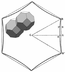
Figure 3: Two semi-regular tetrakaidecahedra superimposed on an illustration of their section from Kelvin’s paper On the Division of Space with Minimum Partitional Area (1887). Real foams do not display such regularity, but their average properties resemble those of the tetrakaidecahedron.

The fundamental difficulty in going beyond this level – and the crucial point of this section – is that while the shaping of domain boundaries is a local process proceeding on the time scale of the underlying interaction, the foam’s evolution, i.e. domain growth, is not. When two domains merge, it is not an isolated event: their nearest neighbors (and then their nearest neighbors, and so on) are also affected, ultimately forcing the whole foam to rebalance. In the case at hand, currents will speed up, slow down or even reverse, taking our charged test particle along on a continued three-dimensional random walk. Since currents live on domain boundaries, we are led to expect the statistical properties of the test particle’s trajectory, i.e. scale invariance and average radius growth according to (38), to carry over to the foam itself.

This does indeed turn out to be the case. After much experimental and numerical work (not least on Potts models, believed to closely approximate the finite temperature dynamics of SU(N) gauge theories in general and of SU(2) in particular wipf2006 ), a consensus has emerged in recent years that the average volume growth rate of three-dimensional domains with $f$ faces is well described by a simple linear dependence on $f$ glazier2000 prause2000

$$\langle V_{f}\rangle^{-1/3}\frac{d\langle V_{f}\rangle}{dt}=\kappa\left(f-f_{0}\right)$$ (40)

whence

$$f_{0}\approx\frac{\langle f^{2}\rangle}{\langle f\rangle}$$ (41)

Empirically, $f_{0}\approx 14\pm 2$, well in line with our guesstimate based on sphere crunching. Growth laws on the form (40) (i.e. with right hand side depending only on the number of faces, or more generally on topological features of the domains) lead to the anticipated time dependence (38) for the average domain radius. This result is also expected on dimensional grounds from the emergence of a scaling state, characterized by growing average domain size but time-independent topological and area distributions mullins1989 , again consistent with expectations from the random walk argument (scale invariance).

The scaling state is a disordered one, not a regular structure composed of individually near-optimal partitions such as Kelvin’s famous 14-faced tetrakaidecahedron (Fig. 3). The discovery by Weaire and Phelan weaire1994 that an 8-cell “repeat unit” with $\langle f\rangle=13.5$ and $\langle n_{e}\rangle=5.11$ achieves a more efficient (smaller total surface) partitioning of a given volume than Kelvin’s solution explains why: a combination of many cells of different shape can actually have lower total surface energy than a regular structure.

It bears emphasizing that these are universal results, depending only on the assumption that the system strives for surface area minimization, not on any details of the underlying interactions. In equation (40), all interaction dependence is encapsulated in the constant $\kappa$. In particular, it can not be underscored enough that the domain boundaries referred to here have nothing in common with topologically stable defects: they do not depend on non-trivial mappings between spacetime and internal degrees of freedom for their existence, they have low energy density, they give rise to a completely different domain structure (the foam), and they positively must be unstable for domain growth and emergence of the scaling state to be at all possible. Domains grow by merging, i.e. by the disappearance of domain boundaries; if the latter were stable, growth could not happen. The separation of time scales and the decelerating evolution embodied in (38) are collective (and essentially geometric) properties of the whole foam, not of individual domain boundaries.

VI Number of domains

In a relativistic setting, (38) must be qualified by the requirement that the speed of light not be exceeded (locally). The simplest ansatz satisfying this condition is

$$\langle r(t)\rangle=\alpha\sqrt{1+\beta^{2}(t-t_{\alpha})}$$ (42)

valid for $t>=t_{\alpha}$, where $t_{\alpha}$ marks the onset of the scaling state,

$$\langle r(t_{\alpha})\rangle=\alpha$$ (43)

with initial growth rate

$$\langle\dot{r}(t_{\alpha})\rangle=\frac{\alpha\beta}{2}\leq 1$$ (44)

and asymptotic growth rate

$$\lim_{t\rightarrow\infty}\langle\dot{r}(t)\rangle=\frac{\alpha\beta}{2\thinspace\sqrt{t}}$$ (45)

Putting (42) on the standard Robertson-Walker metric with scale factor $a(t)$ yields the proper ensemble domain radius

$$\langle r_{RW}(t)\rangle=\frac{a(t)}{a(t_{\alpha})}\thinspace\langle r(t)\rangle+\int_{t_{\alpha}}^{t}d\tau\thinspace\frac{a(\tau)}{a(t_{\alpha})}\thinspace\langle\dot{r}(\tau)\rangle$$ (46)

with

$$\langle\dot{r}(t)\rangle=\frac{\alpha\beta^{2}}{2\sqrt{1+\beta^{2}(t-t_{\alpha})}}$$ (47)

Figure 4: Expected domain boundary redshifts for $\alpha/r_{H}(t_{\alpha})\in[1,10]$, $\langle\dot{r}(t_{\alpha})\rangle=10^{-4}$, $t_{\alpha}=t(z_{\alpha}=1089)$ (recombination) in a flat, dust-matter Friedmann model.

Sweeping $\beta$ over the range $[0,2/\alpha]$ will take us through the possible values of $N_{\Phi}$, the average number of observable $\langle\Phi\rangle$ domains in an arbitrary spatial direction. What can we expect to find?

The limit case $\beta=0$ is easily understood: it describes domains of average size $\alpha$ being effectively “frozen out” at $t=t_{\alpha}$ (by their growth rate becoming negligible compared to that of the universe) and then simply coasting along with their comoving volume. Assuming flatness, if $\alpha$ is the Hubble radius at the time of the EWPT, the opposed effects of subsequent horizon growth and metric expansion work out to $N_{\Phi}\sim 10^{23-15}=10^{8}$. If a freeze-out occurs later, $N_{\Phi}$ can be substantially lower. Section IV suggests $N_{\Phi}\lesssim 10^{5}$. One frozen domain per Hubble radius at recombination, $z\approx 1089$ according to cosmic microwave background (CMB) data, would translate to only $N_{\Phi}\sim 30$ today.

At the other end of the $\beta$ range, the Hubble radius poses an absolute limit. As recently emphasized by Penrose penrose2004 in a revival of the old homogeneity problem of pre-inflationary cosmology, light reaching us now from quasars in opposite directions must have originated in different electroweak domains, as those sources have not been in causal contact since before the EWPT, which occurred well after the end of inflation . Thus,

$$1\lesssim N_{\Phi}\lesssim 10^{8}$$ (48)

As will become evident in Section VII, too small a number, i.e. a rate of realignment too close to the speed of light, would indeed be incompatible with the observed isotropy of the universe.

For a more detailed view, we must turn to equation (46). By isotropy, we should expect an infinite sequence of domain boundaries at (average) proper distances

$$d_{n}(t)=\langle r_{RW}(t)\rangle\thinspace(2n-1)\quad\quad n\in[1,\infty[$$ (49)

What we actually observe is light emitted at time $t_{em}$ and reaching us at time $t$, so

$$\int_{t_{em}}^{t}\frac{d\tau}{a(\tau)}=d_{n}(t_{em})$$ (50)

Given $a(t)$, i.e. a cosmological model, we can solve (50) for $t_{em}$ and plug the result into

$$z=\frac{a(t)}{a(t_{em})}-1$$ (51)

to obtain the observed redshift $z$. In practice, this must be done numerically. See Appendix A for easily adaptable R r2005 code and Fig. 4 for a simple example (but not necessarily an unrealistic one, at least for small $z$): a flat dust-matter model featuring $O(1)$ slow-growing domains per Hubble radius at recombination.

To recap the story so far: while average domain radius is $\propto\sqrt{t}$, the Hubble radius is $\propto t$ (assuming flatness). Therefore, while any finite volume will eventually find itself within a single domain, the number of observable domains grows with time ($\propto\sqrt{t}$, again assuming flatness).

VII Residual luminosity distributions

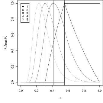
Figure 5: Probability distribution functions $P_{n}(\ell)$ (vertically rescaled) for the residual luminosity $\ell$ after $n$ boundary crossings between $n+1$ domains with independent $\langle\Phi\rangle$.

Imagine a physicist in the $\langle\Phi\rangle$ domain $\mathfrak{D}_{1}$ preparing a pure photon state ${\bm{M}}^{A}_{\mu}$ as defined by (27) and sending it to a colleague in the adjacent domain $\mathfrak{D}_{2}$. To verify the purity of the received ${\bm{M}}_{\mu}$, the colleague performs the operation (24) on it (e.g. by measuring the peak interference amplitude with a locally produced reference state). What will she see?

In their work, both physicists must implicitly rely on their respective, local definition of a photon. The obvious way to distinguish a photon from a $Z^{0}$ is that only the latter has mass, a fact which is made explicit in the electroweak Lagrangian by a change of basis in weak isospin space

$$\langle\Phi\rangle\rightarrow\langle\Phi^{\prime}\rangle=\begin{bmatrix}0\\ \phi_{0}\end{bmatrix}$$ (52)

making $\phi_{0}\in\Re$ the only non-zero component of $\langle\Phi\rangle$. This choice of basis aligns our coordinate axes in weak isospin space with the direction which was picked by the Higgs field at the EWPT. The SU(2)$\times$U(1) (sub)symmetry of the ground state manifold guarantees the existence of a transformation $\bm{U}$, as defined by (28), which achieves this alignment. The Higgs and gauge fields in the new basis are given by (36) and (29), respectively. In this basis, the $Z^{0}$ has a mass term and the photon does not.

But a global SU(2)$\times$U(1) transformation $\bm{U}$ can put $\langle\Phi\rangle$ on the form (52) in only one of the two domains $\mathfrak{D}_{1}$ and $\mathfrak{D}_{2}$. In the other domain, where $\langle\Phi\rangle$ is different, $\bm{U}$ has no particular significance. Therefore, the local definition of a photon is not the same in $\mathfrak{D}_{1}$ and in $\mathfrak{D}_{2}$.

Formally, it is of course possible to perform a local transformation and “gauge away” any misalignment in $\langle\Phi\rangle$ everywhere in the universe, but as we saw in Section IV, only at the cost of using (37) in lieu of (29), i.e. of trading gradients in $\langle\Phi\rangle$ for gradients in ${\bm{M}}_{\mu}(x)$. This amounts to a change of variables and of focus, from the Higgs field inside domains to electrically charged gauge fields across their boundaries. While it may facilitate the description of processes at the boundaries, it does not affect the physics, and it does not help our two physicists somewhere inside their respective domain $\mathfrak{D}_{1}$ and $\mathfrak{D}_{2}$ to establish a common frame of reference in weak isospin space. To that end, they need to exchange photons and literally see what they get. If they choose to analyze the experiment in terms of gauge fields across the boundary, they must integrate along the entire path of the photons; if they choose to think in terms of the Higgs in the bulk, they need only consider the end points of the path.

We can now answer the question asked at the beginning of this section: if the VEVs $\langle\Phi\rangle$ in $\mathfrak{D}_{1}$ and $\mathfrak{D}_{2}$ are related by a transformation with U(1) parameter $\omega_{0}$ and SU(2) parameters ${\bm{\omega}}$, a pure photon state ${\bm{M}}^{A}_{\mu}$ prepared in $\mathfrak{D}_{1}$ will be seen by an observer in $\mathfrak{D}_{2}$ as a mix of $\ell({\bm{\omega}})$ parts photons and $1-\ell({\bm{\omega}})$ parts $Z^{0}$s and $W^{\pm}$s, with $\ell({\bm{\omega}})$ given by (34). Physically, photons crossing the boundary between two electroweak domains are partially converted to weak vector bosons, which then quickly decay to fermions and lower energy photons, leaving us with the residual luminosity $\ell({\bm{\omega}})$.

This is the essence of the problem pointed out by Penrose penrose2004 . If vacuum realignment proceeded at or near the speed of light, we would have only O(1) domain boundaries within our Hubble volume, causing glaring anisotropies. Unless we are prepared to give up locality, the resolution of this apparent contradiction between standard model and observation lies in the opposite direction, i.e. in a subluminal rate of realignment allowing a larger number of domains to even out such anisotropies. (More on this in Section IX).

Since ${\bm{\omega}}$ was picked randomly at the EWPT, the value of $\ell({\bm{\omega}})$ can not be predicted. The best we can hope for is its probability distribution function (PDF). Viewing ${\bm{\omega}}$ as the SU(2) parametrization

$$[n_{0},n_{i}]\to\cos(\omega/2)+i\tau_{i}\frac{\omega_{i}}{\omega}\sin(\omega/2)$$ (53)

of the unit 3-sphere

$$(n_{0})^{2}+(n_{1})^{2}+(n_{2})^{2}+(n_{3})^{2}=1$$ (54)

(the Higgs vacuum manifold, up to a factor $|\langle\Phi\rangle|$) we have

$$\omega/2 = \arccos(n_{0})$$ (55)

$$\omega_{i} = \frac{\omega\thinspace n_{i}}{\sin(\omega/2)}$$ (56)

Substituting Eqs. (55)-(56) into Eq. (34) then yields

$$\ell({\bm{n}})=1-2n_{\bot}^{2}\sin^{2}(\theta_{W})$$ (57)

i.e. luminosity is determined by

$$n_{\bot}^{2}=n_{1}^{2}+n_{2}^{2}$$ (58)

The luminosity PDF therefore follows from that of $n_{\bot}^{2}$ over the unit 3-sphere. For uniformly distributed ${\bm{n}}$, it is simply a step function, $P_{1}(\ell)>0$ for $\ell\in[1-2\sin^{2}(\theta_{W}),1]$.

While the dynamics may modify this result (because the electroweak symmetry group is only a subgroup of the 3-sphere’s O(4)) a uniform ${\bm{n}}$ distribution is the null hypothesis until numerical simulation results become available.

Having obtained the PDF for one domain boundary crossing, $P_{1}(\ell)$, we can easily extend our analysis to the distribution for the residual luminosity $\ell=\ell_{1}\cdot\ell_{2}\cdot...\cdot\ell_{n}$ after $n$ crossings between $n+1$ domains with independent $\langle\Phi\rangle$. By Rohatgi’s result for the distribution of the product of two stochastic variables rohatgi1976 ,

$$P_{2}(\ell=\ell_{1}\cdot\ell_{2})=\int_{\ell}^{1}\thinspace dxP_{1}(x)P_{1}(\ell/x)/x$$ (59)

and generally

$$P_{n+1}(\ell=\ell_{1}\cdot\ell_{2}\cdot...\cdot\ell_{n})=\int_{\ell}^{1}\thinspace dxP_{1}(x)P_{n}(\ell/x)/x$$ (60)

(The argument $\ell/x$ can be shifted around between the two PDFs in the integrand by a trivial change of variables; for numerics, the form shown is preferable, since it minimizes interpolation on the grid at maximum gradient). R code for $P_{n}(\ell)$ is given in Appendix C.

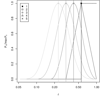
Figure 6: Log-linear version of Fig. 5. $P_{n}(\ell)$ is seen to quickly approach a lognormal shape for $n>3$.

PDFs and cumulative distribution functions for $n\in[1,5]$ are displayed in Fig. 5, 6 and 7. Visually, their most striking feature is the swiftness by which $P_{n}(\ell)$ morphs from a step function for $n=1$ to a lognormal for $n>3$. But the real highlights of this analysis are the first two records in Table 1: they tell us to expect a residual luminosity $\ell\ \sim 0.78\pm 0.13$ for photons moving between adjacent domains, and $\ell\ \sim 0.60\pm 0.14$ for photons crossing two domain boundaries, well in line with the $\ell/\ell_{E}$ ratio of high-$z$ supernovae, $\sim 0.79$.

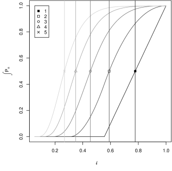
Figure 7: Cumulative probability distribution functions $P_{n}(L\leq\ell)$ for the residual luminosity $\ell$ after $n$ boundary crossings between $n+1$ domains with independent $\langle\Phi\rangle$.

Table 1: Mean, median, standard deviation, skewness and excess kurtosis of $P_{n}(\ell)$ (5000 bins).

$n$	$\langle\ell\rangle$	$\tilde{\ell}$	$\sigma$	$\gamma_{1}$	$\gamma_{2}$
1	0.7774	0.7780	0.1283	0.0082	-2.970378
2	0.6044	0.5904	0.4491	0.3564	-2.949819
3	0.4700	0.4550	0.1362	0.5845	-2.944213
4	0.3655	0.3488	0.1232	0.7681	-2.946776
5	0.2842	0.2678	0.1078	0.9285	-2.953191

VIII Supernova dimming

The state of the art of $\ell/\ell_{E}$ determination is well illustrated by riess2004 , where Riess et.al. quote an intrinsic dispersion for individual supernovae (due to sparse sampling and noisy photometry) of 0.15 magnitudes (in line with e.g. schmidt1998 and filippenko2003 ), and actual dispersions about best fits (on a “gold set” of 157 SNe Ia carefully selected from all available data) of 0.27 magnitudes for $0.1<z<1.0$, increasing to 0.29 magnitudes for $z>1.0$. By the standard magnitude/luminosity relation

$$l_{2}/l_{1}=100^{(m_{1}-m_{2})/5}$$ (61)

this translates to an intrinsic luminosity uncertainty $\pm 100^{0.15/5}\sim\pm 0.15$, with actual $\ell/\ell_{E}$ dispersion ranging all the way from 0.78 to 1.28 for $0.1<z<1.0$, and from 0.77 to 1.31 for $z>1.0$. From these figures, making the (intentionally overoptimistic) assumption that all errors are independent, the 1 $\sigma$ width for the combined $\ell/\ell_{E}$ ratio is $\epsilon\approx 0.25/\sqrt{157}\approx 0.02$, i.e.

$$\ell/\ell_{E}\approx 0.79\pm 0.02$$ (62)

In terms of electroweak domains, the statistics is poorer. Under the null hypothesis that our $\langle\Phi\rangle$ domain is an average one, it has $\sim 14$ nearest neighbor boundaries (see Section V). With high-$z$ supernova searches concentrated to the equatorial plane (so that the evolution of light curves, needed for distance determination, may be tracked from observatories on both hemispheres) we are probably looking through fewer than half of them (see the section drawing in Fig. 3). Based on Table 1, the 1 $\sigma$ expectation width for one boundary crossing is therefore roughly $0.128/\sqrt{7}\approx 0.05$, i.e.

$$\langle\ell_{1}\rangle/\ell_{E}\approx 0.78\pm 0.05$$ (63)

This suggests that there is a single layer of domain boundaries between us and high-$z$ supernovae.

The good match with one domain boundary allows a consistency check: the boundary distance curves of Fig. 4 illustrate the fact that dimming should not start too close to home, lest we end up expecting too many domain boundaries and too dark a universe at higher redshifts. By inspection, the “safe” redshift is $z\gtrsim 0.3$. Ideally (assuming that we are near the center of our domain) we would like to see no sign of dimming at all for lower $z$ than this.

This condition is satisfied: in their 2003 analysis of published SNe Ia data, Padmanabhan and Choudhury padmanabhan2003 found that it split neatly in two subsets about $z=0.25$, consistent with different luminosity zero points and no continuous dimming at all – exactly what crossing of a single domain boundary at $z=0.25$ should look like. Their followup analysis with even more data choudhury2005 showed that the split point can be moved all the way to $z=0.34$ with little consequence, definitely bringing it into our “safe” zone. The conclusion that there is little or no evidence of accelerated expansion for $z\lesssim 0.3$ was again reached by Shapiro and Turner in shapiro2006 .

Summing up, the SNe Ia data appear to fit our expectations well, based only on the standard electroweak and big bang models and without any need for a cosmological constant.

IX Discussion

This paper presents a novel picture of the universe as a foam-like structure of large-scale electroweak domains in a scaling state, arguing that this is both a natural consequence of the standard big bang and electroweak models and a good match to SNe Ia observations – in fact the only one to date sans $\Lambda>0$ .

In this picture, “dark energy” (in the restricted sense of an unseen contribution to $\Omega$) is carried not by a hypothetical new (set of) scalar field(s) with negative pressure, as in the popular quintessence models, but rather by the long wavelength modes of a very familiar one: the standard model Higgs (or the superset of Higgs fields employed by standard model extensions). The SNe Ia luminosity deficit is caused not by accelerated expansion, but by photon conversion at domain boundaries. No exotic new physics is needed. The most “speculative” assumption is that electroweak domain growth is an unexceptional case of generic 3D domain growth.

In the reader’s mind, this picture has likely already been met with a strong objection (if not earlier, then upon review of Fig. 4): what about the CMB? If we live inside an irregular polyhedron with faces of different opacity, should we not see huge anisotropies in the microwave background?

The first part of the answer is a counterquestion: what’s a poor photon to turn into? The $2.73\thinspace K$ of the present-day CMB translate to $2.35\cdot 10^{-4}\thinspace eV$, well below the rest mass of any known particle except the photon and – perhaps – the lightest neutrino. With current neutrino oscillation data indicating mass differences $\gtrsim 10^{-2}\thinspace eV$ melchiorri2005 (plus a much debated claim from the Heidelberg-Moscow double beta decay experiment for $m_{\nu}>0.17\thinspace eV$ klapdor2001 ) conversion of CMB photons may simply be kinematically forbidden, making electroweak domain boundaries effectively transparent to them. In this regime, instead of conversion, photons can be expected to undergo random scattering, resulting in the diffuse glow seen in ordinary foams.

Two bounds on the lightest neutrino mass are thus implied: $m_{\nu}\gtrsim 10^{-4}\thinspace eV$ to prevent readily visible CMB anisotropies, $m_{\nu}\lesssim 1\thinspace eV$ for supernova dimming without the reddening problem of dust models (the optical range being roughly 2 to 3 $eV$). Incidentally, the lower bound also explains an observed discrepancy in the relation between luminosity and angular diameter distances for supernovae and radio sources which has been used to argue against photon loss as an alternative to Hubble acceleration bassett2004 : if domain boundaries are transparent to microwaves, they are necessarily transparent to radio waves, too.

It may be possible to improve the lower bound on $m_{\nu}$ by going back in time, to higher CMB temperatures. If $m_{\nu}\lesssim 0.13\thinspace eV$, Heidelberg-Moscow notwithstanding, we will eventually reach a point along the road to recombination at $0.26\thinspace eV\sim z=1089$ where CMB photons could be converted to neutrinos (the ionization potential of hydrogen is $13.6\thinspace eV$, but recombination occurs later due to photons in the blackbody distribution tail and transitions between excited states). Two considerations then come into play. First, the number of domain boundaries cutting through the equatorial plane at a given distance is roughly proportional to the number of domains out to that distance. The WMAP angular resolution, $\approx 0.3^{\circ}$, is enough to resolve 1200 individual faces, equivalent to $\sim 1200/6=200$ domains. Any $N_{\Phi}\gtrsim 200\cdot 0.26/(2m_{\nu})$ should therefore be safe from direct observation by WMAP. Given $m_{\nu}\lesssim 0.13\thinspace eV$, this implies $N_{\Phi}\gtrsim 200$. It then becomes a question of statistics: how large are the anisotropies caused by differences between (individually unresolvabe) faces?

Fluctuations in primary radiation which was exponentially damped by $O(N_{\Phi})$ boundary crossings are clearly irrelevant: $N_{\Phi}\gtrsim 200$ implies a residual luminosity $\langle\ell\rangle\lesssim 0.78^{200}\sim 10^{-22}$; with $N_{\Phi}=10^{5}$, as suggested by Section IV, $\langle\ell\rangle\sim 10^{-10^{4}}$. Rather, the dominating contributions should be from secondary photons which were redshifted below the $2m_{\nu}$ threshold after only a few boundary crossings. Now, Fig. 6 reminds us that residual luminosity distributions become approximately lognormal, implying constant relative standard deviation, already at $n=3$. To estimate the resulting anisotropies, we can therefore simply read off $\sigma/\langle\ell\rangle\sim 10^{-1}$ from Table 1, invoke the central limit theorem and divide by the square root of the number of faces covered by a pixel at the $2m_{\nu}$ threshold, $N_{0}\approx(2m_{\nu}/0.26)\cdot N_{\Phi}$ domains out.

For a sphere with radius $N_{0}$, the area of a cap subtended by angle $\theta$ is $2\pi N_{0}^{2}(1-\cos(\theta/2))$. Tiling it with tetrakaidecahedra of unit diameter gives us $7/(\pi/4)$ faces per unit area, for a total of $28N_{0}^{2}(1-\cos(\theta/2))$ faces. This is actually an underestimate, since it does not take the uneven spacing of domain boundaries into account; at large $z$, we should rescale the radius by the comoving coordinate distance

$$D(z)=\frac{2\Omega z+(\Omega-2)(\sqrt{1+\Omega z}-1)}{\Omega^{2}(1+z)}$$ (64)

(see e.g. weinberg1972 ) to get

$$N\approx 28\thinspace(N_{0}D(z))^{2}\thinspace(1-\cos(\theta/2))$$ (65)

(another way to see this is to first correct tile size for angular diameter distance and then $N_{0}$ for scale factor). Inserting the WMAP angular resolution $\theta=0.3\cdot\pi/180$, $\Omega=1$, $z=1089\cdot 2m_{\nu}/0.26$, $m_{\nu}=0.1\thinspace eV$ and $N_{\Phi}=10^{5}$ yields fluctuations $\sim 10^{-1}/\sqrt{N}\sim 10^{-5}$, in line with observation. For smaller values, reduce $\Omega$ (everything else being equal, the old preferred $\Omega\approx 0.3$ buys a further factor 1/10) and/or increase $m_{\nu}$ and/or $N_{\Phi}$ (by equation (48) there is plenty of margin here too; the order of magnitude argument pointing to $N_{\Phi}\sim 10^{5}$ is certainly very rough).

While this estimate is already in the right ballpark, keep in mind that it ignores smoothing by random scattering (diffuse glow) and the successive injection of high energy radiation from astrophysical sources. Over time, down-conversion and scattering of this radiation by domain boundaries should also build up a contribution to the CMB. Intuitively, its spectrum should be the unit eigenstate of a Markov chain through the decay channels available at each photon’s energy, with a peak about the average energy of photons produced by the last decay in the chain; essentially the “resonance peak” of the lightest particle capable of decaying to photons (yes, there is a definite iconoclastic possibility lurking in this observation). Computing it should not be hard, given a reliable Monte Carlo generator of highly virtual weak boson decays (alas, apparently not a priority in off-the-shelf simulation packages geared toward high energy experiments).

A detailed CMB calculation would also require all neutrino masses to be specified; the $\alpha$ and $\beta$ parameters of Section VI to be extracted by numerical simulation of the scaling state in the electroweak model under consideration, in turn requiring knowledge of the Higgs mass(es); and of course a consistent choice of cosmological expansion history. It would be a large undertaking, but a systematic exploration of model+parameter space might yield useful constraints on candidate cosmological and/or extended electroweak models.

This resolution of the Penrose conundrum penrose2004 has a problematic implication: the CMB is not quite the fossil we thought it was. Long after it left the surface of “last” scattering, it was interacting with domain boundaries, and later on it may have picked up significant (dominating?) contributions from other sources. This begs the question if it really is telling us so much about the early universe as we currently like to believe. Its large scale isotropy would undeniably be difficult to explain differently, but at smaller angular separations, its features may be of more recent origin. In particular, while none of this directly contradicts inflation (even $\Omega\approx 1$ seems possible to accomodate, at least at this early stage), it does call in question the relevance of the CMB towards testing both inflationary and alternative scenarios khoury2001 luminet2005 .

On the other hand, once the large-scale electroweak foam picture starts sinking in, many new venues of investigation readily suggest themselves. Do domain boundaries balance the energy budget of the universe? What are their effects on structure formation? Can the evidence for dark matter from cosmic shear be reinterpreted in terms of domain boundary effects? Can they help explain observed CMB anomalies magueijo2006 lieu2005 lieu2006 ?

The answers are out there.

Appendix A Domain boundary positions (R code)

# Replace flat dust with pet cosmos here
w <- 0
q <- 2 / (3 * (1 + w))
a <- function(t) { t^q }

# Auxiliary cosmological functions
arecip <- function(t) { 1/a(t) }
dprop <- function(t0, t1) {
   integrate(arecip, t0, t1,
   rel.tol=1E-13, abs.tol=1E-13)$value }
hR <- function(t) { a(t) * dprop(0, t) }

# Compute expected domain redshifts

redshifts <- function(
   a_alpha = 1/1090,  # a(t_alpha)
   r_alpha = 1,       # r(t_alpha)/rH(t_alpha)
   v_alpha = 0.00022, # v(t_alpha)
   maxZ = 5, maxN = 10)
{
   znVector <- array(NaN, c(1, maxN))

   # Domain functions
   r <- function(t) {
      alpha * sqrt(1 + beta2*(t - t_alpha)) }
   integrand <- function(t) {
      0.5 * alpha * beta2 * a(t) /
      sqrt(1 + beta2*(t - t_alpha)) }
   rprop <- function(t)
   {
      integral <- integrate(integrand,
                            t_alpha, t,
                            rel.tol=1E-13,
                            abs.tol=1E-13)
      (a(t) * r(t) + integral$value ) / a_alpha
   }
   dn <- function(t, n) { (2*n - 1) * rprop(t) }

   # Derived parameters
   a_alpha_dev <- function(t_alpha) {
      (a_alpha - a(t_alpha))^2 }
   t_alpha <- optimize(a_alpha_dev,
                       c(0, 1), tol=1E-30)$minimum

   alpha <- hR(t_alpha) * r_alpha
   beta <- 2 * v_alpha / alpha
   beta2 <- beta*beta

   # Main loop

   t_em_dev <- function(t, n) {
      (dprop(t, 1) - dn(t, n))^2 }

   for(n in 1:maxN)
   {
      t_em <- optimize(t_em_dev,
                       c(0, 1), n = n, tol=1E-30)
      z <- a(1)/a(t_em$minimum) - 1
      znVector[n] <- z

      if ((t_em$minimum < t_alpha) ||
          (z > maxZ)) break
   }

   znVector
}

# Main program
redshifts()

Appendix B Luminosity distribution for n = 1 (R code)

sw2 <- 0.22216              # sin^2(theta_W)

oneCrossLuminosity <- function(n)
# Return PDF and CDF of luminosity
# Simple step function for input to nCrossLuminosity()
 {
   pdf <- array(0, c(n))
   cdf <- array(0, c(n))

   i <- round(n*(1.0 - 2.0*sw2))

   pdf[i + 1:(n - i)] <- 1.0/(n - i + 1);

   cdf[1] <- pdf[1]
   for (i in 2:n) { cdf[i] <- pdf[i] + cdf[i-1] }

   # Return results
   list(pdf=pdf, cdf=cdf)
}

# Main program
sample <- sampleLuminosity(5000)
save(sample, file="sample.txt", ascii=TRUE)

Appendix C Luminosity distributions for n $\geq$ 1 (R code)

nCrossLuminosity <- function(maxCross, n1pdf, n1cdf)
# Compute PDF&CDF for 2 to maxCross boundary crossings
{
   n <- length(n1pdf)

   pdf <- array(0, dim=c(maxCross, n))
   cdf <- array(0, dim=c(maxCross, n))

   for (i in 1:n)
   {
      pdf[1, i] <- n1pdf[[i]]
      cdf[1, i] <- n1cdf[[i]]
   }

   if (maxCross > 1)
   {
      for (nCross in 1:(maxCross - 1))
      {
         cumulative <- 0
         for (iy in 1:n)
         {
            integral <- pdf[nCross, n] * n1pdf[iy] / iy

            if (iy < n)
            {
               for (ix in (iy+1):n)
               {
                  integral <-
                     integral +
                     pdf[nCross, (n*iy) %/% ix] *
                     n1pdf[ix]/ix
               }
            }

            integral <- n*integral
            pdf[nCross + 1, iy] <- integral
            cumulative <- cumulative + integral
            cdf[nCross + 1, iy] <- cumulative
         }
      }
   }

   # Return PDFs and CDFs

   list(pdf=pdf, cdf=cdf)
}

# Main program
multi <- nCrossLuminosity(5, sample$pdf, sample$cdf)
save(multi, file="multi.txt", ascii=TRUE)

Table 2: Parameters of fit and error squared $\epsilon^{2}$ for CDF parametrization $F(\ell;a,b,c,d)$ (66).

$n$	$a$	$b$	$c$	$d$	$\epsilon^{2}$
1	0.29650820	0.4238114	-0.1885901	0.05361303	6.011231
2	0.05948206	0.7159291	-0.3665269	0.1868697	-0.03652571
3	0.09153357	-2.05914	72.6966	14.41858	-0.3107125
4	0.01036675	0.3067824	-0.3199721	0.1081582	-0.08748841
5	0.4831496	-2.23015	31.56453	22.18672	-0.05052748

Table 3: Parameters of fit and error squared $\epsilon^{2}$ for PDF parametrization $g(\ell;a,b,c,d,e)$ (71).

$n$	$a$	$b$	$c$	$d$	$e$	$\epsilon^{2}$
1	2.484335e-05	-0.1780371	0.2699788	5.571233e-08	0.0002125698	8.168009e-05
2	1.198534e-06	-0.5352473	0.2612992	-1.576451e-07	0.0001519190	9.103221e-05
3	1.897927e-07	-0.6941752	0.332284	-2.835761e-08	0.0003936519	-0.0003655848
4	8.499097e-08	-0.9647373	0.3736279	-1.269617e-08	0.0003422317	-0.0003472561
5	5.919239e-08	-1.235350	0.4105253	-1.767185e-08	0.0003091985	-0.0003447646

Appendix D Distribution fits

For $n>1$, the CDFs $P_{n}(L\leq\ell)$ of Fig. 7 are found to be well parameterized by

$$F(\ell;a,b,c,d)=\frac{F_{ln}(\ell^{a};b,c)\thinspace\exp(d\thinspace\ell^{a})}{F_{ln}(1;b,c)\thinspace\exp(d)}$$ (66)

where $F_{\ln}(x;b,c)$ is the lognormal CDF

$$F_{\ln}(x;b,c)\equiv\frac{1}{2}\left\{1+{\rm erf}\left(\frac{\ln(x-b)}{c\sqrt{2}}\right)\right\}$$ (67)

${\rm erf}(x)$ is the error function

$${\rm erf}(x)\equiv\frac{2}{\sqrt{\pi}}\int_{0}^{x}dy\thinspace\exp(-y^{2})$$ (68)

and the parameters $a,b,c,d$ (plus total error squared $\epsilon^{2}$) obtained on a 5000$\times$5000 point grid are given in Table 2.

Differentiating (66) in $\ell$ yields the corresponding parametrization of $P_{n}(\ell)$:

$$f(\ell;a,b,c,d)\equiv\frac{d}{dx}F(\ell;a,b,c,d)=$$

$$\frac{\left(f_{ln}(\ell^{a};b,c)+d\thinspace F_{ln}(\ell^{a};b,c)\right)\thinspace\exp(d\thinspace\ell^{a})\thinspace ax^{a-1}}{F_{ln}(1;b,c)\thinspace\exp(d)}$$ (69)

where $f_{ln}(x;b,c)$ is the lognormal PDF,

$$f_{ln}(x;b,c)\equiv\frac{1}{2cx\sqrt{2\pi}}\exp\left({-\frac{\left(\ln{x}-b\right)^{2}}{2c^{2}}}\right)$$ (70)

For the first couple of $n$, fitting directly on $P_{n}(\ell)$ with

$$g(\ell;a,b,c,d,e)\equiv f_{ln}(\ell;a,b)\left\{\frac{c}{1-x}+d+ex\right\}$$ (71)

achieves a better reproduction of the sharp peak dominating the PDF. Parameters obtained on a 5000$\times$5000 point grid are given in Table 3.

References

- (1) A.G. Riess et al (1998) Astron. J. 116, 1009.
- (2) S. Perlmutter et al (1998) Nature (London) 391, 51-54.
- (3) S. Perlmutter et al (1999) Astrophys. J. 517, 565.
- (4) B. Schmidt et al (1998) Astrophys. J. 507, 46-63.
- (5) A. Filippenko (2003) in Carnegie Observatories Astrophysics Series, Vol. 2: Measuring and Modeling the Universe, ed. W. L. Freedman (Cambridge University Press, Cambridge) (http://arxiv.org/astro-ph/0307139).
- (6) A.G. Riess et.al. (2004) Astrophys. J. 607, 665-687 (http://arxiv.org/abs/astro-ph/0402512).
- (7) B.E. Schaefer (2006) Astrophys. J., in press (http://arxiv.org/abs/astro-ph/0612285).
- (8) A. Blanchard, M. Douspis, M. Rowan-Robinson, S. Sarkar (2003) Astron. Astrophys. 412, 35-44 (http://arxiv.org/abs/astro-ph/0304237).
- (9) A.Z. Bonanos et al (2006) Astrophys. J. 652, 313 (http://arxiv.org/abs/astro-ph/0606279).
- (10) L. Wang, D. Baade, F. Patat (2006) Science, in press (http://arxiv.org/abs/astro-ph/0611902).
- (11) S.L. Glashow (1961) Nucl. Phys. 22, 579.
- (12) S. Weinberg (1967) Phys. Rev. Lett. 19, 1264.
- (13) A. Salam (1968) in Elementary Particle Physics (Nobel Symp No. 8), ed. N. Svartholm (Almqvist and Wiksell, Stockholm).
- (14) G. ’t Hooft (1971) Nucl. Phys. B33, 173.
- (15) G. ’t Hooft (1971) Nucl. Phys. B35, 167.
- (16) P.W. Higgs (1964) Phys. Rev. Lett. 13, 509.
- (17) P.W. Higgs (1966) Phys. Rev. 145, 1156.
- (18) T. Anderberg (2008) arxiv:0804.2284 (http://arxiv.org/abs/0804.2284).
- (19) M. Dine, A. Kusenko (2004) Rev. Mod. Phys. 76, 1 (http://arxiv.org/abs/hep-ph/0303065).
- (20) M. Trodden (1999) Rev. Mod. Phys. 71, 1463-1500 (http://arxiv.org/abs/hep-ph/9803479).
- (21) G.D. Moore (2000) JHEP 0003, 006 (http://arxiv.org/abs/hep-ph/0001274).
- (22) H. Kurki-Suonio, M. Laine (1996) Phys. Rev. Lett. 77, 3951-3954 (http://arxiv.org/abs/hep-ph/9607382).
- (23) K. Kajantie, M. Laine, K. Rummukainen, M. Shaposhnikov (1996) Phys. Rev. Lett. 77, 2887-2890 (http://arxiv.org/abs/hep-ph/9605288).
- (24) F. Csikor, Z. Fodor, J. Heitger (1999) Phys. Rev. Lett. 82, 21-24 (http://arxiv.org/abs/hep-ph/9809291).
- (25) N. Turok (1989) Phys. Rev. Lett. 63, 2625.
- (26) T. Anderberg (2007) arxiv:0711.3187 (http://arxiv.org/abs/0711.3187).
- (27) N. Turok, J. Zadrozny (1990) Phys. Rev. Lett. 65, 2331.
- (28) J. Schwinger (1951), Phys. Rev. 82, 664.
- (29) A.D. Dolgov, F.R. Urban (2005) Astropart. Phys. 24, 289-300 (http://arxiv.org/abs/hep-ph/0505255).
- (30) M. Nagasawa, R. Brandenberger (2003) Phys. Rev. D67, 043504 (http://arxiv.org/abs/hep-ph/0207246).
- (31) T.W.B. Kibble (1976) J. Phys. A9, 1387.
- (32) J.A. Harvey, E.W. Kolb, D.B. Reiss, S. Wolfram (1982) Nucl. Phys. B201, 16.
- (33) T. Vachaspati, A. Vilenkin (1984) Phys. Rev. D30, 2036.
- (34) N. Graham (2007) Phys. Rev. Lett. 98, 101801; ibid. 189904(E) (http://arxiv.org/abs/hep-th/0610267).
- (35) H.S.M. Coxeter (1958) Illinois J. Math. 2, 746-758.
- (36) H.S.M. Coxeter (1961) in Introduction to Geometry, 2nd ed., 405-411 (Wiley, New York).
- (37) B. Kleihaus, J. Kunz, K. Myklevoll (2004) Phys. Lett. B582, 187-195 (http://arxiv.org/abs/hep-th/0310300).
- (38) J. von Neumann (1952) Metal Interfaces, 108 (American Society for Metals, Cleveland).
- (39) J.A.F. Plateau (1873) Statique Experiméntal et Théorique des Liquides Soumis aux Seules Forces Moléculaires (Gauthier-Villars, Paris).
- (40) A. Wipf et.al. (2006) in “O’Raifeartaigh Symposium on Non-Perturbative and Symmetry Methods in Field Theory” (proceedings) (http://arxiv.org/abs/hep-lat/0610043).
- (41) J.A. Glazier, B. Prause (2000) in Foams, Emulsions and their Applications: Current Status of Three-Dimensional Growth Laws, 120-127, ed. P. Zitha, J. Banhart, G. Verbist (Verlag MIT Publishing, Bremen) (http://biocomplexity.indiana.edu/jglazier/papers.php?action=view&cat=02a&id=60).
- (42) B.A. Prause (2000) Magnetic Resonance Imaging of Structure and Coarsening in Three-Dimensional Foams (Ph.D. thesis, University of Notre Dame) (http://biocomplexity.indiana.edu/jglazier/papers.php?action=view&cat=02a&id=81).
- (43) W.W. Mullins, J. Viñals (1989) Acta metall. 37, 991.
- (44) D. Weaire, R. Phelan (1994) Phil. Mag. Lett. 69, 107-110.
- (45) R. Penrose (2004) The Road to Reality, 744-746 (Knopf, New York).
- (46) R Development Core Team (2005) R: A language and environment for statistical computing (Vienna, ISBN 3-900051-07-0) (http://www.R-project.org).
- (47) V.K. Rohatgi (1976) An Introduction to Probability Theory and Mathematical Statistics (Wiley, New York).
- (48) T. Padmanabhan, T.R. Choudhury (2003), MNRAS, 344, 823.
- (49) T.R. Choudhury, T. Padmanabhan (2005) Astron. Astrophys. 429, 807 (http://arxiv.org/abs/astro-ph/0311622).
- (50) C. Shapiro, M.S. Turner, Astrophys. J. 649 (2006) 563 (http://arxiv.org/abs/astro-ph/0512586).
- (51) A. Melchiorri et.al. (2005) Nucl. Phys. B Suppl., Vol. 145, 290-294 (http://arxiv.org/abs/astro-ph/0501531).
- (52) H.V. Klapdor-Kleingrothaus et.al. (2001) Mod. Phys. Lett. A 16, 2409.
- (53) B.A. Bassett, M. Kunz (2004) Astrophys. J. 607, 661-664 (http://arxiv.org/abs/astro-ph/0311495).
- (54) J. Evslin, M. Fairbairn (2006) JCAP 0602, 011 (http://arxiv.org/abs/hep-ph/0507020).
- (55) S. Weinberg (1972) Gravitation and Cosmology, 485 (Wiley, New York).
- (56) J. Khoury, B.A. Ovrut, P.J. Steinhardt, N. Turok (2001) Phys. Rev. D64, 123522 (http://arxiv.org/abs/hep-th/0103239).
- (57) J.P. Luminet (2005) Phys. World 18, 22-28 (http://arxiv.org/abs/physics/0509171).
- (58) J. Magueijo, R.D. Sorkin, astro-ph/0604410 (http://arxiv.org/abs/astro-ph/0604410).
- (59) R. Lieu, J.P.D. Mittaz (2005) Astrophys. J. 628, 583-593 (http://arxiv.org/abs/astro-ph/0412276).
- (60) R. Lieu, J.P.D. Mittaz, S.-N. Zhang (2006) Astrophys. J. 648, 176 (http://arxiv.org/abs/astro-ph/0510160).