The investigation of ELAIS field by Vega photometry: Absolute - magnitude dependent on the Galactic model parameters

Abstract

We estimate the density laws of the Galactic stellar populations as a function of absolute magnitude in a near-polar Galactic field. The density laws are determined by the direct fit to photometric parallaxes from Vega photometry in the ELAIS ($\alpha=16^{h}10^{m}00^{s},\delta=+54^{o}30^{{}^{\prime}}00{{}^{\prime\prime}}$; $l=84^{o}.27$, $b=+44^{o}.90$; 6.571 deg²; epoch 2000) field both independently for each population and simultaneously for all stellar populations. Stars have been separated into different populations based on their spatial location. The thick disc and halo best fit by an exponential. However, the thin disc best fits by using a sech² law for stars at faint absolute magnitudes, $10<M(g^{{}^{\prime}})\leq 11$, $11<M(g^{{}^{\prime}})\leq 12$ and $12<M(g^{{}^{\prime}})\leq 13$, whereas an exponential law for stars at relatively bright absolute magnitudes, $5<M(g^{{}^{\prime}})\leq 6$, $6<M(g^{{}^{\prime}})\leq 7$, $7<M(g^{{}^{\prime}})\leq 8$, $8<M(g^{{}^{\prime}})\leq 9$ and $9<M(g^{{}^{\prime}})\leq 10$. The scaleheights for the sech² density laws are the equivalent exponential scaleheights. Galactic model parameters are absolute magnitude dependent: The scaleheight for thin disc decreases monotonically from stars at bright absolute magnitudes $[M(g^{{}^{\prime}})=5]$ to stars at faint absolute magnitudes $[M(g^{{}^{\prime}})=13]$ in the range 363-163 pc, except the minimum H=211 pc at $9<M(g^{{}^{\prime}})\leq 10$ where sech density law fits better. Its local density is flat at bright absolute magnitudes but it increases at faint absolute magnitudes. For thick disc, the scaleheight is flat within the uncertainties. The local space density of thick disc relative to the local space density for the thin disc is almost flat at absolute magnitude intervals $5<M(g^{{}^{\prime}})\leq 6$ and $6<M(g^{{}^{\prime}})\leq 7$, 7.59 and 7.41 per cent respectively, whereas it decreases down to 3.31 per cent at absolute magnitude interval $7<M(g^{{}^{\prime}})\leq 8$. The axial ratio for the halo is $\kappa$ =0.60, 0.73 and 0.78 for the absolute magnitude intervals $4<M(g^{{}^{\prime}})\leq 5$, $5<M(g^{{}^{\prime}})\leq 6$ and $6<M(g^{{}^{\prime}})\leq 7$ respectively, and its local space density relative to the local space density for the thin disc is 0.06 and 0.04 per cent for the intervals $5<M(g^{{}^{\prime}})\leq 6$, and $6<M(g^{{}^{\prime}})\leq 7$ respectively (the local space density relative to the thin disc could not be derived for the absolute magnitude interval $4<M(g^{{}^{\prime}})\leq 5$ due to the lack of the local space density for thin disc for this interval). The simultaneous fit of all three stellar populations agrees within uncertainties with the most recent values in the literature. Also, each parameter is close to one of the corresponding parameters estimated for different absolute magnitude intervals in this work with one exception however; i.e. the scaleheight for thick disc is relatively small and its error is rather large ($H=760^{+62}_{-55}$ pc).

Table 1: Previous Galactic models. Symbols: TN denotes the thin disc, TK denotes the thick disc, S denotes the spheroid (halo), $R_{e}$ is the effective radius and $\kappa$ is the axes ratio. The figures in the parentheses for Siegel et al. (2002) are the corrected values for binarism. The asterisk denotes the power-law index replacing $R_{e}$.

H (TN)	h (TN)	n (TK)	H (TK)	h (TK)	n (S)	$R_{e}$ (S)	$\kappa$	Reference
(pc)	(kpc)		(kpc)	(kpc)		(kpc)
310-325	—	0.0125-0.025	1.92-2.39	—	—	—	—	Yoshii (1982)
300	—	0.02	1.45	—	0.0020	3.0	0.85	Gilmore & Reid (1983)
325	—	0.02	1.3	—	0.0020	3.0	0.85	Gilmore (1984)
280	—	0.0028	1.9	—	0.0012	—	—	Tritton & Morton (1984)
200-475	—	0.016	1.18-2.21	—	0.0016	—	0.80	Robin & Crézé (1986)
300	—	0.02	1.0	—	0.0010	—	0.85	del Rio & Fenkart (1987)
285	—	0.015	1.3-1.5	—	0.0020	2.36	Flat	Fenkart et al. (1987)
325	—	0.0224	0.95	—	0.0010	2.9	0.90	Yoshii, Ishida & Stobie (1987)
249	—	0.041	1.0	—	0.0020	3.0	0.85	Kuijken & Gilmore (1989)
350	3.8	0.019	0.9	3.8	0.0011	2.7	0.84	Yamagata & Yoshii (1992)
290	—	—	0.86	—	—	4.0	—	von Hippel & Bothun (1993)
325	—	0.0225	1.5	—	0.0015	3.5	0.80	Reid & Majewski (1993)
325	3.2	0.019	0.98	4.3	0.0024	3.3	0.48	Larsen (1996)
250-270	2.5	0.056	0.76	2.8	0.0015	2.44-2.75*	0.60-0.85	Robin et al. (1996); Robin, Reylé & Crézé(2000)
290	4.0	0.059	0.91	3.0	0.0005	2.69	0.84	Buser, Rong & Karaali (1998, 1999)
240	2.5	0.061	0.79	2.8	—	—	0.60-0.85	Ojha et al. (1999)
330	2.25	0.065-0.13	0.58-0.75	3.5	0.0013	—	0.55	Chen et al. (2001)
280(350)	2-2.5	0.06-0.10	0.7-1.0 (0.9-1.2)	3-4	0.0015	—	0.50-0.70	Siegel et al. (2002)
320	—	0.07	0.64	—	0.0013	—	0.58	Du et al. (2003)
265-495	—	0.052-0.095	0.80-0.97	—	0.0002-0.0015	—	0.70	Karaali, Bilir & Hamzaoğlu (2004)

1 Introduction

Galactic models have a long history. Bahcall & Soneira (1980) fitted their observations with a double component Galactic model, namely disc and halo, whereas Gilmore & Reid (1983) could succeed to fit their observations with a Galactic model only by introducing a third component, i.e. thick disc. It should be noted that the third component was a rediscovery of the “Intermediate Population II” first described in the Vatican Proceedings review of O’Connel (1958). The new model is discussed by Gilmore & Wyse (1985) and Wyse & Gilmore (1986). Galactic models have been an attractive topic for many research centers, due to their importance: Galactic models can be used as a tool to reveal the formation and evolution of the Galaxy. For some years there has been a conflict among the researchers about the history of our Galaxy. The pioneering work was the one of Eggen, Lynden-Bell & Sandage (1962) who argued that the Galaxy collapsed in a free-fall time ($\sim 2\times 10^{8}$ yr). Now, we know that the Galaxy collapsed over many Gyr (e.g. Yoshii & Saio 1979; Norris, Bessel & Pickles 1985; Norris 1986; Sandage & Fouts 1987; Carney, Latham & Laird 1990; Norris & Ryan 1991; Beers & Sommer-Larsen 1995) and at least some of its components are formed from the merger or accretion of numerous fragments, such as dwarf-type galaxies (cf. Searle & Zinn 1978, Freeman & Bland-Hawthorn 2002, and references therein).

The researchers use different methods to determine the parameters. Table 1 summaries the results of these works. One can see that there is an evolution for the numerical values of model parameters. The local space density and the scaleheight of the thick disc can be given as an example. The evaluations of the thick disc have steadily moved toward shorter scaleheights (from 1.45 to 0.65 kpc, Gilmore & Reid 1983; Chen et al. 2001) and higher local densities (2-10 per cent). In many studies the range of values for the parameters is large. For example, Chen et al. (2001) and Siegel et al. (2002) give 6.5-13 and 6-10 per cent, respectively, for the local space density for the thick disc. However, one expected the most evolved numerical values for these recent works. That is, either the range for this parameter should be small or a single value with a small error should be given for it. It seems that they could not choose the most appropriate procedures in this topic. In fact, we cited in our previous paper (Karaali, Bilir & Hamzaoğlu 2004, hereafter KBH) that the Galactic model parameters are mass dependent. Absolute magnitude is reasonable proxy for mass, therefore they vary at different absolute magnitude intervals. Hence, the parameters cited by the researchers up to recent years which are based on star counts cover the range of a series of parameters corresponding to different absolute magnitude intervals, therefore either their range or their errors are large. Additionally, as it was cited in our previous paper (KBH), sech² density law fits better to the observed density functions for stars with absolutely faint magnitudes, $10<M(g^{{}^{\prime}})\leq 13$, for the thin disc. We aim to use these experiences in the investigation of this field and compare the results with those obtained in the field SA 114, almost symmetric relative to the Galactic plane. It should be noted that evaluations of photometric parallax (Gilmore & Reid 1983, Reid & Majewski 1993, Siegel et al. 2002) have usually broken the fits down by absolute magnitude ranges. More importantly, the Besançon group (e.g. Robin et al. 1996) uses very sophisticated models that create multiple thin disc populations through population synthesis. This is a much more elegant and nuanced way of fitting star count parameters. However, we should mention that the method of photometric parallax is, by necessity, a simplified way of evaluating star counts.

2 The density law forms

Disc structures are usually parameterized in cylindrical coordinates by radial and vertical exponentials,

$$\tiny D_{i}(x,z)=n_{i}exp(-z/H_{i})exp(-(x-R_{0})/h_{i})$$ (1)

where $z$ is the distance from Galactic plane, $x$ is the planar distance from the Galactic center, $R_{0}$ is the solar distance to the Galactic center (8.6 kpc, Buser et al. 1998), $H_{i}$ and $h_{i}$ are the scaleheight and scalelength respectively, and $n_{i}$ is the normalized local density. The suffix $i$ takes the values 1 and 2, as long as the thin and thick discs are considered. It should be noted that the sophisticated models of Besançon and others use multiple thin discs to account for the range of populations (e.g. Robin et al. 1996). A similar form uses the sech² (or sech) function to parameterize the vertical distribution for the thin disc,

$$D_{1}(x,z)=n_{1}sech^{2}(-z/H^{{}^{\prime}}_{1})exp(-(x-R_{o})/h_{1}).$$ (2)

As the secans hyperbolicus is the sum of two exponentials, $H^{{}^{\prime}}_{1}$ is not really a scaleheight but has to be compared to $H_{1}$ by dividing it with 2: $H_{1}=H^{{}^{\prime}}_{1}/2$. We would like to mention that the reason of using a sech² law is due to theoretic analysis which indicate that the density laws should follow a sech² law for an isothermal sheet.

The density law for the spheroid component is parameterized in different forms. The most common is the de Vaucouleurs (1948) spheroid used to describe the surface brightness profile of elliptical galaxies. This law has been deprojected into three dimensions by Young (1976) as

$$D_{s}(R)=n_{s}~{}exp[-7.669(R/R_{e})^{1/4}]/(R/R_{e})^{7/8},$$ (3)

where $R$ is the (uncorrected) Galactocentric distance in spherical coordinates, $R_{e}$ is the effective radius and $n_{s}$ is the normalized local density. $R$ has to be corrected for the axial ratio $\kappa=c/a$,

$$R=[x^{2}+(z/\kappa)^{2}]^{1/2},$$ (4)

where,

$$z=r\sin b,$$ (5)

$$x=[R_{o}^{2}+r^{2}\cos^{2}b-2R_{0}r\cos b\cos l]^{1/2},$$ (6)

$r$ being the distance along the line of sight and, $b$ and $l$ the Galactic latitude and longitude respectively, for the field under investigation. The form used by the Basle group is independent of effective radius but is dependent on the distance from the Sun to the Galactic centre:

$$D_{s}(R)=n_{s}~{}exp[10.093(1-R/R_{o})^{1/4}]/(R/R_{o})^{7/8};$$ (7)

and alternative formulation is the power law,

$$D_{s}(R)=n_{s}/(a_{o}^{n}+R^{n})$$ (8)

where $a_{o}$ is the core radius.

Equations (1) and (2) can be replaced by eqs (9) and (10) respectively, as long as the vertical direction is considered, where

$$D_{i}(z)=n_{i}exp(-z/H_{i}),$$ (9)

$$D_{1}(z)=n_{1}sech^{2}(-z/H_{1}^{{}^{\prime}}).$$ (10)

3 The procedure used in this work

In this work, we used the same procedure cited in our previous paper (KBH), i.e. we compared the derived and theoretical space densities per absolute magnitude interval, in the vertical direction of the Galactic plane for a large absolute magnitude interval $4<M(g^{{}^{\prime}})\leq 13$, down to the limiting magnitude $g^{{}^{\prime}}_{0}=20.5$: (i) we separated the stars into different populations by their spatial position, as a function of both absolute and apparent magnitude; (ii) we tried the exponential and sech² laws for comparison of the derived and theoretical space densities for the thin disc and we found that a sech² law worked better at magnitudes $10<M(g^{{}^{\prime}})\leq 13$ whereas an exponential density law favors at magnitudes $4<M(g^{{}^{\prime}})\leq 10$. This was also the case in our previous paper (KBH); (iii) we derived model parameters for each population individually and for each absolute magnitude interval we observed their differences; and (iv) the model parameters were estimated by comparison of the derived vertical space densities with the combined density laws (eqs. 7 and 9) for stars of all populations. In the last process, we obtained two sets of parameters: one for the absolute magnitude interval $4<M(g^{{}^{\prime}})\leq 10$ and the other $4<M(g^{{}^{\prime}})\leq 13$. As we argued in our previous paper, the different behavior of the faint stars may produce different values and large ranges for parameters derived in starcount studies.

4 The data and reductions

4.1 Observations

The ELAIS field ($\alpha=16^{h}10^{m}00^{s},\delta=+54^{o}30^{{}^{\prime}}00{{}^{\prime\prime}}$; $l=84^{o}.27$, $b=+44^{o}.90$; 6.571 deg²; epoch 2000) was measured by the Isaac Newton Telescope (INT) Wide Field Camera (WFC) mounted at the prime focus ($f/3$) of the 2.5-m INT on La Palma, Canary Islands, during seven observing runs, namely 1999 April 17; 1999 June 7, 9; 1999 July 16-22; 1999 August 1-3, 7, 10, 13, 16-17; 1999 September 7-9; 1999 October 3-5, and 2000 June 24-25. The WFC consists of 4 EVV42 CCDs, each containing 2k $\times$ 4k pixels. They are fitted in a L-shaped pattern which makes the camera have 6k $\times$ 6k pixels, minus a corner of 2k $\times$ 2k pixels. The WFC has 13.5$\mu$ pixels corresponding to 0.33 arcsec pixel^-1 at the INT prime focus, and each covers an area of 22.8 $\times$ 11.4 arcmin² on the sky. This field contains 54 sub-fields and each sub-field covers 4 CCDs with a total area of 0.29 deg². Therefore, the total area of each telescope pointing is 54 $\times$ 0.29 deg² minus the overlapping area. In our work, the data of only 33 sub-fields could be used. Hence, the area of the field investigated is 33 $\times$ 0.29 deg² minus the overlapping area = 6.571 deg². With a typical seeing of 1.0-1.3 arcsec on the INT, point objects are well sampled, which allows accurate photometry.

Observations were taken in five bands ($u^{{}^{\prime}}_{RGO}$, $g^{{}^{\prime}}$, $r^{{}^{\prime}}$, $i^{{}^{\prime}}$, $z^{{}^{\prime}}_{RGO}$, where RGO denotes the Royal Greenwich Observatory) with a single exposure of 600 s to nominal 5$\sigma$ limiting magnitudes of 23, 25, 24, 23, and 22 respectively (McMahon et al. 2001). However, the limiting magnitudes are brighter when stars are considered only. In our work, we determined the $g^{{}^{\prime}}_{0}$ limiting magnitude for stars by estimating from the star count roll over in Fig. 2 as $g^{{}^{\prime}}_{0}=20.5$. Magnitudes are put on a standard scale using observations of ELAIS standard system corresponding to Landolt system , taken on the same night. The accuracy of the preliminary photometric calibrations is $\pm$0.1 mag. The CCD observations are reduced to the magnitudes by the INT WAS group. Three sets of two-colour diagrams, i.e. $(u^{{}^{\prime}}-g^{{}^{\prime}},g^{{}^{\prime}}-r^{{}^{\prime}})$, $(g^{{}^{\prime}}-r^{{}^{\prime}},r^{{}^{\prime}}-i^{{}^{\prime}})$ and $(r^{{}^{\prime}}-i^{{}^{\prime}},i^{{}^{\prime}}-z^{{}^{\prime}})$, for 21 sub-fields show considerable deviations due to bad reduction hence, we left them out of the program. The following processes have been applied to the data for the remaining 33 sub-fields to obtain a sample of stars with new data available for a model parameterization.

4.2 The overlapping sources, de-reddening of the magnitudes, bright stars, and extra-galactic objects

The data of ELAIS field are provided from the Cambridge Astronomical Survey Unit (CASU) . In total, there are 17041 sources in 33 sub-fields in the ELAIS field. It turned out that 3027 of these sources are overlapped, i.e. their angular distances are less than 1 arcsec to any other source. We omitted them, and so the sample reduced to 14014. The $E(B-V)$ colour excess for the sample sources are evaluated by the procedure of Schlegel, Finkbeiner & Davis (1998).

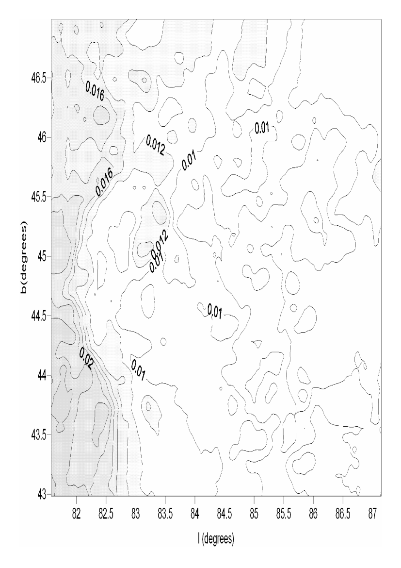
Figure 1: $E(B-V)$ colour-excess contours for the field ELAIS as a function of Galactic latitude and longitude.

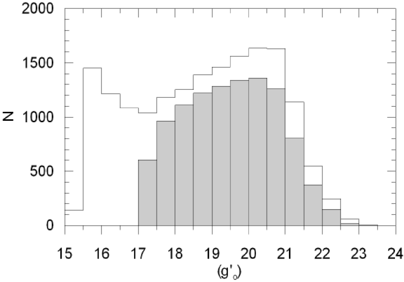
Figure 2: An apparent magnitude histogram for all sources (white colour) and for only the star sample (black colour).

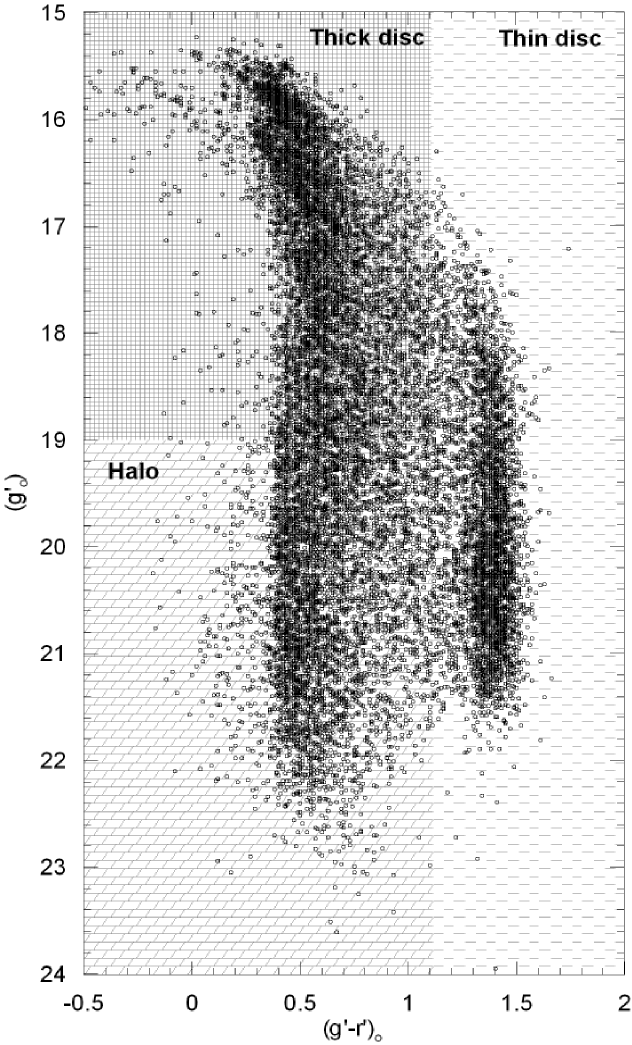
Figure 3: Colour-apparent magnitude diagram for the original sample. The shaded areas for the regions that correspond to each stellar population is indicated.

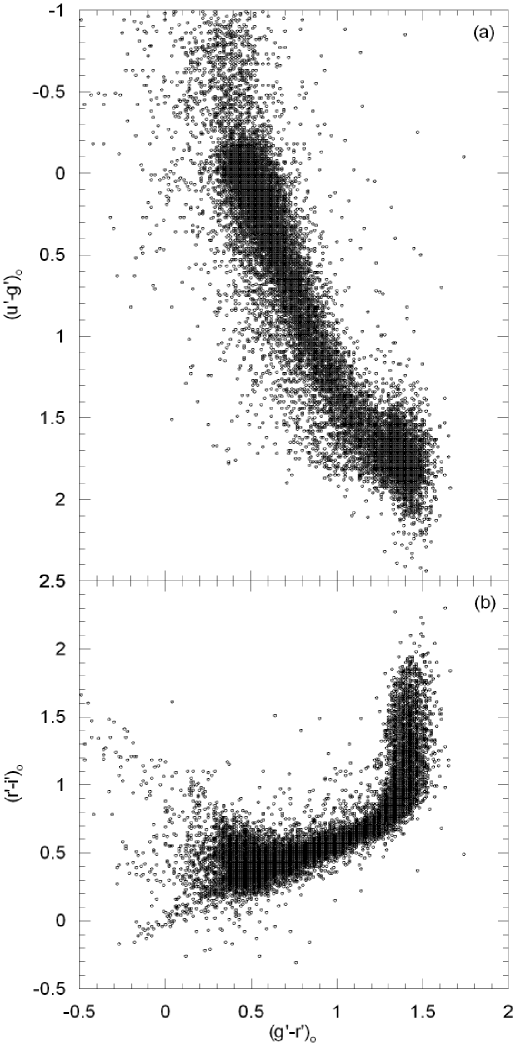
Figure 4: Two-colour diagrams for sources with apparent magnitude $17<g^{{}^{\prime}}_{0}\leq 22$: (a) for $(u^{{}^{\prime}}-g^{{}^{\prime}})_{0}-(g^{{}^{\prime}}-r^{{}^{\prime}})_{0}$ and (b) for ($g^{{}^{\prime}}-r^{{}^{\prime}})_{0}-(r^{{}^{\prime}}-i^{{}^{\prime}})_{0}$.

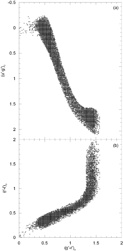
Figure 5: Two-colour diagrams for stars with apparent magnitude. $17<g^{{}^{\prime}}_{0}\leq 22$: (a) for $(u^{{}^{\prime}}-g^{{}^{\prime}})_{0}-(g^{{}^{\prime}}-r^{{}^{\prime}})_{0}$ and (b) for ($g^{{}^{\prime}}-r^{{}^{\prime}})_{0}-(r^{{}^{\prime}}-i^{{}^{\prime}})_{0}$.

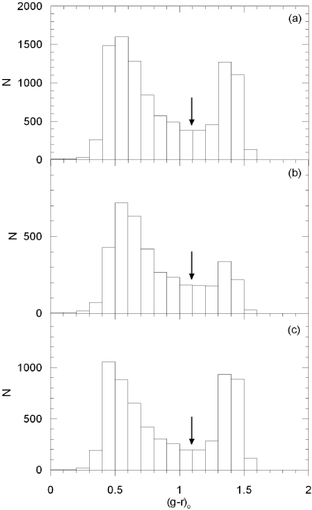
Figure 6: A $(g^{{}^{\prime}}-r^{{}^{\prime}})_{0}$ colour histogram as a function of apparent magnitude, for the star sample: (a) for $17<g^{{}^{\prime}}_{0}\leq 22$, (b) for $17<g^{{}^{\prime}}_{0}\leq 19$ and (c) for $19<g^{{}^{\prime}}_{0}\leq 22$. The vertical downward arrow shows the limit value $(g^{{}^{\prime}}-r^{{}^{\prime}})_{0}=1.1$ mag which separates the thin disc and the thick disc-halo couple.

The $E(B-V)$ colour-excess contours for the field are given in Fig. 1 as a function of Galactic latitude and longitude. Then, the total absorption $A_{V}$ is evaluated by means of the well known equation

$$R_{V}=\frac{A_{V}}{E(B-V)}=3.1.$$ (11)

For Vega bands we used the $R_{\lambda}/R_{V}$ data of Cox (2000) for the interpolation, where $\lambda$ = 3581, 4846, 6240, 7743, and 8763$\AA$, and derived $R_{\lambda}$ from their combination of this with $A_{V}$ (see Table 2, KBH). Finally, the dereddened $u_{0}^{{}^{\prime}}$, $g_{0}^{{}^{\prime}}$, $r_{0}^{{}^{\prime}}$, $i_{0}^{{}^{\prime}}$, and $z_{0}^{{}^{\prime}}$ magnitudes were obtained from the original magnitudes and the corresponding $R_{\lambda}$.

The histogram for the dereddened apparent magnitude $g_{0}^{{}^{\prime}}$ (Fig. 2) and the colour-apparent magnitude diagram (Fig. 3) shows that there is a large number of saturated sources in our sample. Hence, we excluded sources brighter than $g_{0}^{{}^{\prime}}=17$ (this bright limit of apparent magnitude matches with the one claimed in our previous paper, KBH). However, the two-colour diagrams $(u^{{}^{\prime}}-g^{{}^{\prime}})_{0}-(g^{{}^{\prime}}-r^{{}^{\prime}})_{0}$ and $(g^{{}^{\prime}}-r^{{}^{\prime}})_{0}-(r^{{}^{\prime}}-i^{{}^{\prime}})_{0}$ in Fig. 4 indicate that there are also some extragalactic objects, where most of them lie towards the blue as claimed by Chen et al. (2001) and Siegel et al. (2002). As claimed in our paper cited above, the star/extragalactic object separation based on the “stellarity parameter” as returned from the SEXTRACTOR routines (Bertin & Arnouts 1996) could not be sufficient. We adopted the simulation of Fan (1999) in addition to the work cited above, to remove the extragalactic objects in our field. Thus we rejected the sources with $(u^{{}^{\prime}}-g^{{}^{\prime}})_{0}<-0.10$ and those which lie outside of the band concentrated by most of the sources. After the last process, the number of 6.2 per cent sources in the sample-stars-reduced to 10492. The two-colour diagrams $(u^{{}^{\prime}}-g^{{}^{\prime}})_{0}-(g^{{}^{\prime}}-r^{{}^{\prime}})_{0}$ and $(g^{{}^{\prime}}-r^{{}^{\prime}})_{0}-(r^{{}^{\prime}}-i^{{}^{\prime}})_{0}$ for the final sample are given in Fig. 5. A few dozen stars with $(u^{{}^{\prime}}-g^{{}^{\prime}})_{0}\sim-0.10$ and $(g^{{}^{\prime}}-r^{{}^{\prime}})_{0}\sim 0.20$ are probably stars of spectral type A.

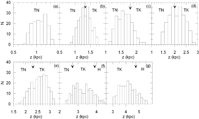
Figure 7: Spatial location for stars with absolute magnitude $6<M(g^{{}^{\prime}})\leq 7$ as a function of apparent magnitude: (a)(17.0,17.5], (b) (17.5,18.0], (c)(18.0,18.5], (d)(18.5,19.0], (e)(19.0,19.5], (f)(19.5,20.0] and (g)(20.0,20.5]. The arrows correspond to the distances from the Galactic plane separating the populations (TN: thin disc, TK: thick disk and H: halo).

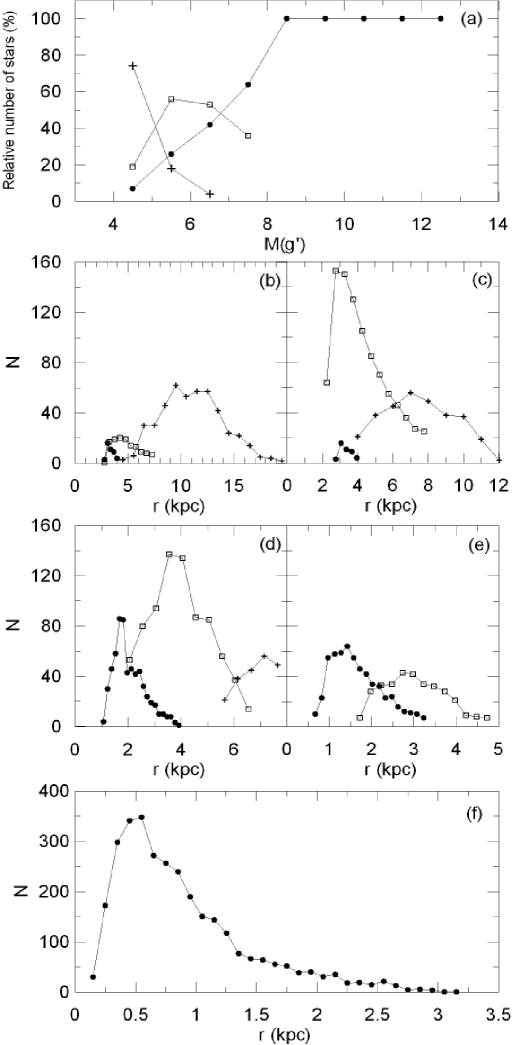
Figure 8: Absolute magnitude ranges dominated by different populations (panel a) and the break of these contributions down by distance bins for the absolute magnitudes $4<M(g^{{}^{\prime}})\leq 5$, $5<M(g^{{}^{\prime}})\leq 6$, $6<M(g^{{}^{\prime}})\leq 7$, $7<M(g^{{}^{\prime}})\leq 8$ and $8<M(g^{{}^{\prime}})\leq 13$ in panels (b), (c), (d), (e) and (f) respectively. Symbols: a plus denotes a halo, a square denotes a thick disc and a filled circle denotes a thin disc.

Table 2: Dominant regions for three populations: the thin disc, the thick disc and the halo, as a function of absolute and apparent magnitudes. The symbol $z$ is the distance to the Galactic plane in kpc.

$M(g^{{}^{\prime}})$	$g_{o}^{{}^{\prime}}$	Thin disc	Thick disc	Halo
(12,13]	(17.0,20.5]	$z\leq 0.34$	$-$	$-$
(11,12]	(17.0,20.5]	$z\leq 0.55$	$-$	$-$
(10,11]	(17.0,20.5]	$z\leq 0.88$	$-$	$-$
(9,10]	(17.0,20.5]	$z\leq 1.40$	$-$	$-$
(8,9]	(17.0,20.5]	$z\leq 2.24$	$-$	$-$
(7,8]	(17.0,18.0]	$z\leq 1.09$	$-$	$-$
	(18.0,18.5]	$z\leq 1.27$	$z>1.27$	$-$
	(18.5,19.0]	$z\leq 1.34$	$z>1.34$	$-$
	(19.0,19.5]	$z\leq 1.60$	$z>1.60$	$-$
	(19.5,20.0]	$z\leq 1.95$	$z>1.95$	$-$
	(20.0,20.5]	$z\leq 2.32$	$z>2.32$	$-$
(6,7]	(17.0,17.5]	$z\leq 1.40$	$-$	$-$
	(17.5,18.0]	$z\leq 1.38$	$z>1.38$	$-$
	(18.0,18.5]	$z\leq 1.80$	$z>1.80$	$-$
	(18.5,19.0]	$z\leq 1.95$	$z>1.95$	$-$
	(19.0,19.5]	$z\leq 2.30$	$z>2.30$	$-$
	(19.5,20.0]	$z\leq 2.70$	$2.70<z\leq 3.90$	$z>3.90$
	(20.0,20.5]	$-$	$z\leq 4.70$	$z>4.70$
(5,6]	(17.0,17.5]	$z\leq 1.55$	$z>1.55$	$-$
	(17.5,18.0]	$z\leq 1.80$	$1.80<z\leq 2.50$	$z>2.50$
	(18.0,18.5]	$z\leq 2.20$	$2.20<z\leq 2.90$	$z>2.90$
	(18.5,19.0]	$z\leq 2.64$	$2.64<z\leq 3.55$	$z>3.55$
	(19.0,19.5]	$-$	$z\leq 4.25$	$z>4.25$
	(19.5,20.0]	$-$	$z\leq 5.00$	$z>5.00$
	(20.0,20.5]	$-$	$z\leq 5.25$	$z>5.25$
(4,5]	(17.0,17.5]	$z\leq 2.20$	$z>2.20$	$-$
	(17.5,18.0]	$z\leq 2.65$	$2.65<z\leq 3.10$	$z>3.10$
	(18.0,18.5]	$z\leq 3.00$	$3.00<z\leq 4.20$	$z>4.20$
	(18.5,19.0]	$-$	$z\leq 4.43$	$z>4.43$
	(19.0,19.5]	$-$	$z\leq 5.20$	$z>5.20$
	(19.5,20.5]	$-$	$-$	$z>5.00$

4.3 Absolute magnitudes, distances, population types and density functions

In the Sloan Digital Sky Survey ($SDSS$) photometry, the blue stars in the range $15<g^{*}<18$ are dominated by thick-disc stars with a turn-off $(g^{*}-r^{*})\sim 0.33$, and for $g^{*}>18$, the Galactic halo, which has a turn-off colour $(g^{*}-r^{*})\sim 0.2$, becomes significant. Red stars $(g^{*}-r^{*})\geq 1.3$, are dominated by thin-disc stars for all apparent magnitudes (Chen et al. 2001). We used the same procedure to demonstrate the three populations (Fig. 3) and to determine the absolute magnitudes for stars in each population by appropriate colour-magnitude diagrams. In our case, the apparent magnitude which separates the thick disc and halo stars seems to be a bit fainter relative to the $SDSS$ photometry, i.e. $g^{{}^{\prime}}_{0}\sim 19$, and the colour separating the red and bluer stars is slightly more blue, i.e. $(g^{{}^{\prime}}-r^{{}^{\prime}})_{0}=1.1$ (Fig. 6). The absolute magnitudes of thick disc and halo stars are evaluated by means of the colour-magnitude diagrams of 47 Tuc ([Fe/H]=-0.65 dex, Hesser et al. 1987) and M13 ([Fe/H]=-1.40 dex, Richer & Fahlman 1986) respectively, whereas for thin disc stars we used the colour-magnitude diagram of Lang (1992) for population I stars. The colours and absolute magnitudes in the $UBV$ system were converted to ELAIS photometry as follows: We used two equations for colour transformations from the WEB page of CASU:

$$g^{{}^{\prime}}-r^{{}^{\prime}}=0.908(B-V)+0.048,$$ (12)

$$g^{{}^{\prime}}-B=-0.531(B-V)+0.053.$$ (13)

The first equation transforms $B-V$ to $g^{{}^{\prime}}-r^{{}^{\prime}}$ colour. The second equation can be written in the following form which provides $M(g^{{}^{\prime}})$ absolute magnitudes:

$$M(g^{{}^{\prime}})=M(B)-0.531(B-V)+0.053.$$ (14)

The $M(B)$ absolute magnitudes in eq. 14 were evaluated either by eq. 15 (for the data of Lang, 1992) or by eq. 16 (for the data of clusters 47 Tuc and M13):

$$M(B)=M(V)+(B-V),$$ (15)

$$M(B)=B-(V-M(V))_{0},$$ (16)

where $(V-M(V))_{0}$ is the distance modules of the cluster in question. The distance to a star relative to the Sun is carried out by the following formula:

$$[g^{{}^{\prime}}-M(g^{{}^{\prime}})]_{o}=5\log r-5.$$ (17)

The vertical distance to the Galactic plane ($z$) of a star could be evaluated by its distance $r$ and its Galactic latitude ($b$) which could be provided by its right ascension and declination.

The precise separation of stars into different populations has been carried out by their spatial positions as a function of their absolute and apparent magnitudes. The procedure is based on the histograms for distance $z$ from the Galactic plane. Fig. 7 gives the histograms for stars with $6<M(g^{{}^{\prime}})\leq 7$ for the apparent $g^{{}^{\prime}}_{0}$ magnitude intervals $17<g^{{}^{\prime}}_{0}\leq 17.5$, $17.5<g^{{}^{\prime}}_{0}\leq 18$, $18<g^{{}^{\prime}}_{0}\leq 18.5$, $18.5<g^{{}^{\prime}}_{0}\leq 19$, $19<g^{{}^{\prime}}_{0}\leq 19.5$, $19.5<g^{{}^{\prime}}_{0}\leq 20$ and $20<g^{{}^{\prime}}_{0}\leq 20.5$ as an example. The vertical arrows show the position that the number of stars decline. The distance $z$ corresponding these positions are adopted as the borders of three populations of the Galaxy, i.e. they limit the efficiency regions of the populations.

This topic can be clarified in more detail as follows: The dominance regions of thin disc, thick disc and halo are at short, intermediate, and large $z$ distances respectively. The number counts for thin disc decreases with increasing $z$ distance, whereas for thick disc the number counts are very small at short $z$ distances, then they increase at intermediate $z$ distances. The decreasing or increasing rate is not the same for the two populations. The same case is valid for thick disc and halo at large $z$ distances. Hence, statistically, there should be drops in the number counts at population transitions. This technique first used in the paper of Karaali (1994). He showed that the $z$-histograms for three populations show a multimodal distribution where the modes at short, intermediate and large $z$ distances correspond to thin disc, thick disc and halo stars respectively. As shown by Karaali, the agreement of the kinematical distribution of the sample stars with their spatial location is a strong confirmation of the technique in question.

The technique improved in the recent years (cf. KBH) by introducing the apparent magnitude of stars used in the histograms. A population breaks at higher $z$-distances when one goes to faint apparent magnitudes, and there are histograms where the statistical fluctuations are rather small relative to the deeps at the population transitions. These two arguments are the clues in the separation of stars into different population types, i.e. thin and thick discs and halo. However, any wrong identification of a genuine drop reflects in the value of the parameter in question and its corresponding error.

Table 3: The logarithmic space density function $D^{*}=\log D+10$, for different absolute magnitude intervals for the thin disc. $r^{*}=[(r^{3}_{1}+r^{3}_{2})/2]^{1/3}$ is the centroid distance for the volume $\Delta V_{1,2}$, and $z^{*}=r^{*}\sin b$, ($b$) being the Galactic latitude of the field center. The other symbols are explained in the text (distances in kpc, volumes in pc³).

$M(g^{{}^{\prime}})\rightarrow$				(4,5]		(5,6]		(6,7]		(7,8]		(8,9]		(9,10]		(10,11]		(11,12]		(12,13]
$r_{1}-r_{2}$	$\Delta V_{1,2}$	r*	z*	N	D*	N	D*	N	D*	N	D*	N	D*	N	D*	N	D*	N	D*	N	D*
0.10-0.20	4.67 (3)	0.16	0.12															11	7.37	19	7.61
0.20-0.30	1.27 (4)	0.26	0.18											2	6.20	36	7.45	90	7.85	49	7.59
0.30-0.40	2.47 (4)	0.36	0.25											20	6.91	129	7.72	118	7.68	35	7.15
0.40-0.60	1.01 (5)	0.52	0.37									22	6.34	126	7.09	284	7.45	238	7.37	13	6.11
0.60-0.80	1.97 (5)	0.71	0.50							16	5.91	132	6.83	91	6.66	238	7.08	71	6.56
0.80-1.00	3.26 (5)	0.91	0.64							53	6.21	165	6.70	90	6.44	170	6.72
1.00-1.25	6.36 (5)	1.14	0.80					21	5.52	107	6.23	184	6.46	112	6.25	68	6.03
1.25-1.50	9.49 (5)	1.37	0.98					73	5.89	93	5.99	113	6.08	81	5.93
1.50-1.75	1.32 (6)	1.64	1.15			13	4.99	130	5.99	88	5.82	114	5.94	33	5.40
1.75-2.00	1.76 (6)	1.88	1.33			86	5.69	122	5.84	68	5.59	100	5.75	5	4.45
2.00-2.50	5.09 (6)	2.28	1.61			167	5.52	138	5.43	86	5.23	117	5.36
2.50-3.00	7.59 (6)	2.77	1.96	11	4.16	94	5.09	72	4.98	48	4.80	52	4.84
3.00-3.50	1.06 (7)	3.27	2.31	21	4.30	51	4.68	40	4.58	22	4.32
3.50-4.00	1.41 (7)	3.77	2.66	9	3.81	26	4.27	20	4.15
4.00-4.50	1.81 (7)	4.26	3.01	4	3.34
Total				45		437		616		581		999		560		925		528		116

Table 4: The logarithmic space density function, $D^{*}=\log D+10$, for different absolute magnitude intervals for the thick disc. Symbols as in Table 3.

$M(g^{{}^{\prime}})\rightarrow$				(4,5]		(5,6]		(6,7]		(7,8]
$r_{1}-r_{2}$	$\Delta V_{1,2}$	r*	z*	N	D*	N	D*	N	D*	N	D*
1.0-1.5	1.58 (6)	1.30	0.92
1.5-2.0	3.09 (6)	1.78	1.26					16	4.71	30	4.99
2.0-2.5	5.09 (6)	2.28	1.61			64	5.10	80	5.20	70	5.14
2.5-3.0	7.59 (6)	2.77	1.96	1	3.12	153	5.30	73	4.98	69	4.96
3.0-3.5	1.06 (7)	3.27	2.31	17	4.21	150	5.15	111	5.02	75	4.85
3.5-4.0	1.41 (7)	3.77	2.66	10	3.85	130	4.96	148	5.02	46	4.51
4.0-4.5	1.81 (7)	4.26	3.01	23	4.10	105	4.76	103	4.76	26	4.16
4.5-5.0	2.26 (7)	4.76	3.36	19	3.92	85	4.58	89	4.60	10	3.65
5.0-5.5	2.76 (7)	5.26	3.71	15	3.74	70	4.40	79	4.46
5.5-6.0	3.31 (7)	5.76	4.07	12	3.56	55	4.22	46	4.14
6.0-6.5	3.91 (7)	6.26	4.42	9	3.36	46	4.07	27	3.84
6.5-7.0	4.56 (7)	6.76	4.77	7	3.19	36	3.90	5	3.04
7.0-8.0	1.13 (8)	7.53	5.32	9	2.90	25	3.35
8.0-9.0	1.45 (8)	8.53	6.02			27	3.27
Total				122		946		777		326

Table 2 gives the full set of absolute and apparent magnitude intervals and the efficiency regions of the populations. The distance over which a population, the thin disc for example, dominates increases with declining absolute magnitude. That is, the three populations are not squeezed into small isolated volumes. The same holds also when one goes to apparently faint magnitudes in an absolute magnitude interval. These findings were cited also in our previous paper (KBH) and are consistent with the results of Reid & Majewski (1993), who argued that the thick disc extends up to $z\sim 4$ kpc, a distance from the Galactic plane where halo stars cannot be omitted. Halo stars dominate the absolutely bright intervals, thick disc stars indicate the intermediate brightness intervals and thin disc stars indicate the faint intervals, as expected (Fig. 8a). If we break these contributions down by distance bins, we would reveal that the efficient region for each population shifts to shorter distances relative to the Sun, when one goes from absolutely bright to absolutely faint magnitudes (Fig. 8b-f). For example, thin disc is efficient at $r\sim 1.5$ kpc for the absolutely magnitudes $6<M(g^{{}^{\prime}})\leq 7$ and $7<M(g^{{}^{\prime}})\leq 8$ whereas the efficiency shifts to $r\sim 0.5$ kpc for the interval $8<M(g^{{}^{\prime}})\leq 13$.

Table 5: The logarithmic space density function, $D^{*}=\log D+10$, for different absolute magnitude intervals for the halo. Symbols as in Table 3.

$M(g^{{}^{\prime}})\rightarrow$				(4,5]		(5,6]		(6,7]
$r_{1}-r_{2}$	$\Delta V_{1,2}$	r*	z*	N	D*	N	D*	N	D*
3-4	1.41 (7)	3.77	2.66			11	3.89
4-6	1.01 (8)	5.19	3.66	9	2.95	75	3.87	24	3.37
6-8	1.97 (8)	7.14	5.04	60	3.48	95	3.68	41	3.32
8-10	3.26 (8)	9.11	6.43	108	3.52	90	3.44
10-15	1.58 (9)	12.98	9.16	231	3.16	34	2.33
15-17.5	1.32 (9)	16.35	11.54	41	2.49
Total				449		305		65

The logarithmic density functions, $D^{*}=\log D+10$, are given in Tables 3-5 and Figures 9-11 for different absolute magnitudes for three populations, where: $D=N/\Delta V_{1,2}$; $\Delta V_{1,2}=(\pi/180)^{2}(\sq/3)(r_{2}^{3}-r_{1}^{3})$; $\sq$ denotes the size of the field (6.571 deg²); $r_{1}$ and $r_{2}$ denote the limiting distance of the volume $\Delta V_{1,2}$; $N$ denotes the number of stars (per unit absolute magnitude); $r^{*}=[(r^{3}_{1}+r^{3}_{2})/2]^{1/3}$ is the centroid distance for the volume $\Delta V_{1,2}$; and $z^{*}=r^{*}\sin b$, ($b$) being the Galactic latitude of the field center. The horizontal thick lines, in Tables 3-5, corresponding to the limiting distance of completeness ($z_{l}$) are evaluated by the following equations:

$$[g^{{}^{\prime}}-M(g^{{}^{\prime}})]_{o}=5\log r_{l}-5,$$ (18)

$$z_{l}=r_{l}\sin b,$$ (19)

where $g_{0}^{{}^{\prime}}$ is the limiting apparent magnitude (17 and 20.5 for the bright and faint stars respectively), $r_{l}$ the limiting distance of completeness relative to the Sun and $M(g^{{}^{\prime}})$ is the appropriate absolute magnitude $M_{1}$ or $M_{2}$ for the absolute magnitude interval $M_{1}-M_{2}$ considered.

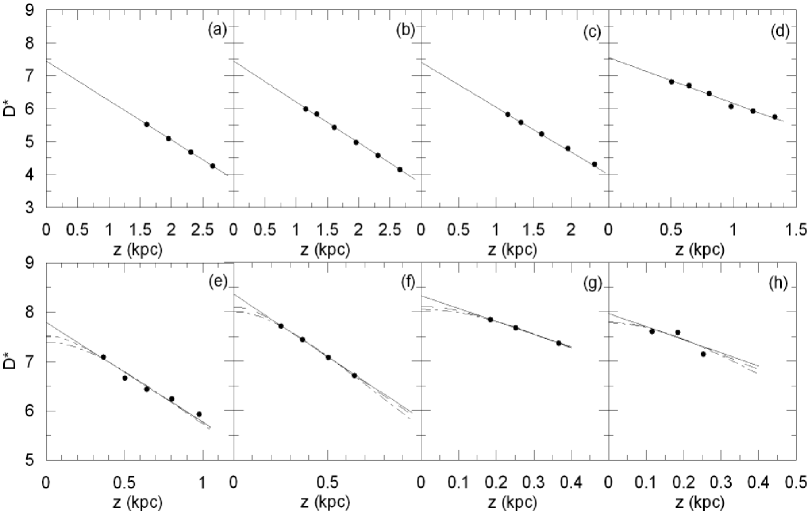
Figure 9: Comparison of the observed space density function with the density laws for different absolute magnitude intervals for the thin disc. (a) (5,6], (b) (6,7], (c) (7,8], (d) (8,9], (e) (9,10], (f) (10,11], (g) (11,12] and (h) (12,13]. The continuous curve represents the exponential law, the dashed curve, represents the $sech$ law and dashed-dot curve represents the sech² law.

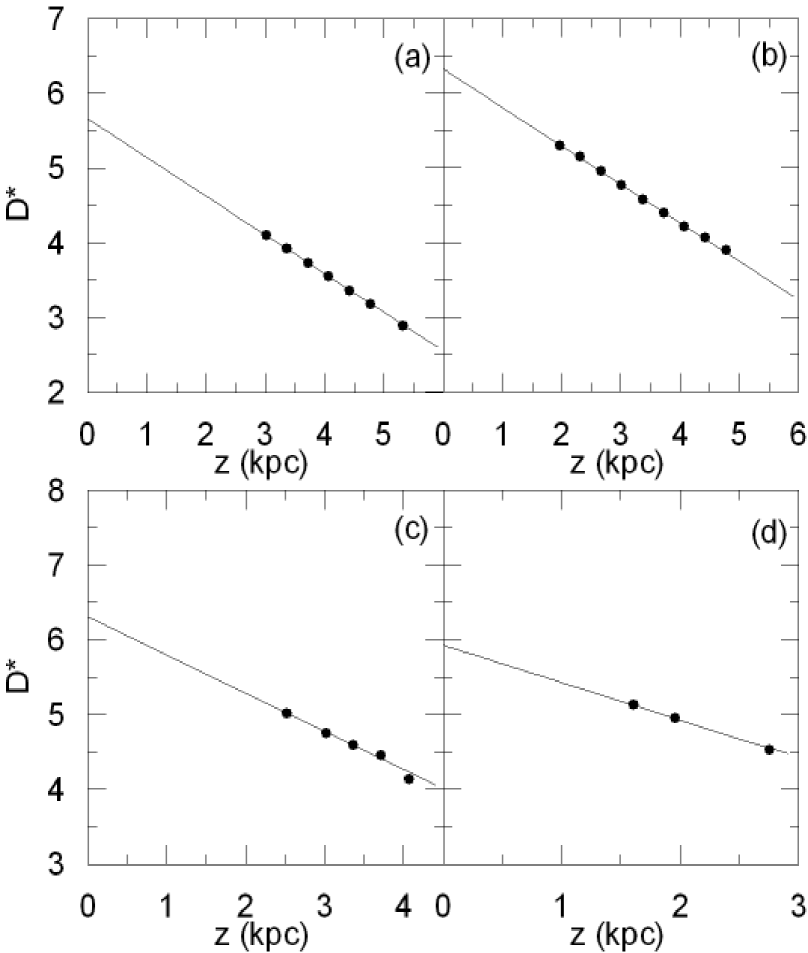
Figure 10: Comparison of the derived space density function with the exponential density law for different absolute magnitude intervals for the thick disc. (a) (4,5], (b) (5,6], (c) (6,7] and (d) (7,8].

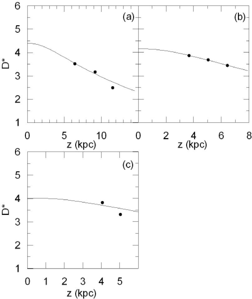
Figure 11: Comparison of the derived space density function with the de Vaucouleurs density law for different absolute magnitude intervals for the halo. (a) (4,5], (b) (5,6] and (c) (6,7].

We acknowledge that in this work we have used a simple method. We have postulated mono-metallic stellar populations with no abundance gradient, and we have not applied any correction for binarism, contamination by compact galaxies or giant/sub-giants neither. We are making a simplified evaluation.

Table 6: Galactic model parameters for different absolute magnitude intervals for the thin disc resulting from the comparison of observed logarithmic space densities with a (unique) density law (Fig. 9). The columns give: absolute magnitude interval $M(g^{{}^{\prime}})$, the density law, the logarithmic local space density $n^{*}$, scaleheight for sech or sech² density law $H_{1}^{{}^{\prime}}$ (in the parenthesis), the scaleheight for exponential density law $H$, $\chi^{2}_{min}$, the standard deviation $s$ and the local space density for $Hipparcos$ $\odot$.

$M(g^{{}^{\prime}})$	Density law	$n^{*}$	$(H_{1}^{{}^{\prime}})~{}~{}H$	$\chi^{2}_{min}$	$s$	$\odot$
(12,13]	exp	$7.97^{+0.10}_{-0.10}$	$163^{+42}_{-28}$	7.33	$\pm$ 0.13	8.05
	sech	$7.80^{+0.09}_{-0.09}$	$(227)~{}~{}137^{+31}_{-22}$	6.42	0.10
	sech2	$7.78^{+0.09}_{-0.09}$	$(428)~{}~{}214^{+45}_{-31}$	5.70	0.11
(11,12]	exp	$8.33^{+0.01}_{-0.01}$	$167^{+1}_{-1}$	0.09	0.01	7.92
	sech	$8.11^{+0.01}_{-0.01}$	$(254)~{}~{}153^{+1}_{-1}$	0.01	0.00
	sech2	$8.05^{+0.01}_{-0.01}$	$(514)~{}~{}257^{+3}_{-2}$	0.07	0.01
(10,11]	exp	$8.36^{+0.01}_{-0.01}$	$172^{+1}_{-2}$	0.58	0.01	7.78
	sech	$8.10^{+0.01}_{-0.01}$	$(275)~{}~{}166^{+1}_{-2}$	0.13	0.01
	sech2	$8.00^{+0.01}_{-0.01}$	$(590)~{}~{}295^{+2}_{-3}$	0.55	0.01
(9,10]	exp	$7.79^{+0.07}_{-0.07}$	$216^{+14}_{-13}$	16.90	0.09	7.63
	sech	$7.52^{+0.07}_{-0.07}$	$(350)~{}~{}211^{+16}_{-13}$	19.48	0.09
	sech2	$7.39^{+0.08}_{-0.08}$	$(770)~{}~{}385^{+35}_{-28}$	25.95	0.11
(8,9]	exp	$7.55^{+0.05}_{-0.05}$	$313^{+15}_{-13}$	12.70	0.06	7.52
(7,8]	exp	$7.41^{+0.02}_{-0.02}$	$318^{+3}_{-3}$	1.59	0.04	7.48
(6,7]	exp	$7.44^{+0.03}_{-0.03}$	$351^{+6}_{-6}$	2.49	0.03	7.47
(5,6]	exp	$7.44^{+0.01}_{-0.01}$	$363^{+1}_{-1}$	0.03	0.01	7.47

5 Galactic model parameters

We estimated Galactic model parameters by comparison of the derived space density functions, with the density laws both independently for each population as a function of absolute magnitude and simultaneously for all stellar populations.

5.1 Absolute magnitude dependent Galactic model parameters

The thin disc density laws were fitted with the additional constraint of producing local densities consistent with those derived from $Hipparcos$ (Jahreiss & Wielen 1997), a procedure applied in our previous paper (KBH). It was discovered that the sech² law fitted better for the intervals $10<M(g^{{}^{\prime}})\leq 11$ and $11<M(g^{{}^{\prime}})\leq 12$ confirming our results in our paper mentioned above, however, contrary to our expectation, the exponential law fitted better for the interval $12<M(g^{{}^{\prime}})\leq 13$ and the sech law fitted better for the interval $9<M(g^{{}^{\prime}})\leq 10$, whereas the exponential law was favourite in our previous paper (KBH, Table 6 and Fig. 9). The comparison for absolutely bright intervals, i.e. $8<M(g^{{}^{\prime}})\leq 9$, $7<M(g^{{}^{\prime}})\leq 8$, $6<M(g^{{}^{\prime}})\leq 7$ and $5<M(g^{{}^{\prime}})\leq 6$ is carried out with the exponential law, as in our previous paper cited above. The scaleheight for thin disc increases monotonically from 163 to 363 pc when one goes from the absolute magnitude interval $12<M(g^{{}^{\prime}})\leq 13$ to $5<M(g^{{}^{\prime}})\leq 6$, with the exception scaleheight H=211 pc for the interval $9<M(g^{{}^{\prime}})\leq 10$ which is less than the one for the interval $10<M(g^{{}^{\prime}})\leq 11$, i.e. H=295 pc. As cited above, $9<M(g^{{}^{\prime}})\leq 10$ is the unique absolute magnitude interval where sech density law fitted better with the derived space densities in our work, and it is a transition interval between those for which either exponential law (for bright intervals) or sech² law (for fainter intervals) fitted better. All scaleheights are equivalent to the exponential law scaleheights. The local space density for thin disc, for different absolute magnitude intervals, is consistent with the $Hipparcos^{\prime}$ one (Table 6).

For the thick disc, the derived logarithmic space density functions are compared with the exponential density law for the absolute magnitude intervals $7<M(g^{{}^{\prime}})\leq 8$, $6<M(g^{{}^{\prime}})\leq 7$, $5<M(g^{{}^{\prime}})\leq 6$ and $4<M(g^{{}^{\prime}})\leq 5$, (Table 7 and Fig. 10). The range for the scaleheight is rather small, 839-867 pc and the scaleheight itself is flat within the quoted uncertainties. The local space density relative to the local space density of thin disc ($n_{2}/n_{1}$) could not be given for the interval $4<M(g^{{}^{\prime}})\leq 5$ due to lack of local space density for this interval for the thin disc. For the intervals $5<M(g^{{}^{\prime}})\leq 6$ and $6<M(g^{{}^{\prime}})\leq 7$, $n_{2}/n_{1}$ is 7.59 and 7.41 per cent respectively, equivalent to the updated numerical values, whereas for the faintest interval, $7<M(g^{{}^{\prime}})\leq 8$, $n_{2}/n_{1}$=3.31 per cent is close to the original value (Gilmore & Wyse 1985).

The derived logarithmic space density functions for the halo are compared with the de Vaucouleurs density law for the absolute magnitude intervals $6<M(g^{{}^{\prime}})\leq 7$, $5<M(g^{{}^{\prime}})\leq 6$ and $4<M(g^{{}^{\prime}})\leq 5$ (Table 8 and Fig. 11). The local space density relative to the thin disc ($n_{3}/n_{1}$) could not be given for the interval $4<M(g^{{}^{\prime}})\leq 5$ due to the reason cited above. For the intervals $6<M(g^{{}^{\prime}})\leq 7$ and $5<M(g^{{}^{\prime}})\leq 6$, $n_{3}/n_{1}$=0.04 and 0.06 per cent respectively. The numerical values for the axial ratio $\kappa$ for two intervals are close to each other, i.e. $\kappa=0.78$ and $\kappa=0.73$ for $6<M(g^{{}^{\prime}})\leq 7$ and $5<M(g^{{}^{\prime}})\leq 6$ respectively, but a bit less for the interval $4<M(g^{{}^{\prime}})\leq 5$, $\kappa=0.60$, consistent with the previous ones within the uncertainties however.

The parameters derived for three populations have been tested by the luminosity function (Fig. 12), where $\varphi^{*}(M)$ is the total of the local space densities for three populations. The local space densities for the thick disc and the halo are presented in Table 9. The local space densities of $Hipparcos$ were converted to ELAIS colours by the combination of eqs (13) and (15) which give the following relation between $M(g^{{}^{\prime}})$ and $M(V)$ absolute magnitudes:

$$M(g^{{}^{\prime}})=M(V)+0.469(B-V)+0.053$$ (20)

There is a good agreement between our luminosity function and that of $Hipparcos$ (Jahreiss & Wielen 1997). Also the error bars are rather short. We used the procedure of Phleps et al. (2000) for the error estimation in Tables 6-8 (above) and Tables 13 and 14 (in the following sections), i.e. changing the values of the parameters until $\chi^{2}_{min}$ increases or decreases by 1.

Table 7: Galactic model parameters for the thick disc. $n_{2}/n_{1}$ indicates the local space density for the thick disc relative to the thin disc. Other symbols are same as in Table 6.

$M(g^{{}^{\prime}})$	$n^{*}$	$H$ (pc)	$\chi^{2}_{min}$	$s$	$n_{2}/n_{1}$ (per cent)
(7,8]	$5.93^{+0.03}_{-0.03}$	$867^{+24}_{-21}$	0.32	$\pm$ 0.05	3.31
(6,7]	$6.31^{+0.03}_{-0.03}$	$849^{+14}_{-16}$	2.88	0.05	7.41
(5,6]	$6.32^{+0.01}_{-0.01}$	$845^{+9}_{-7}$	0.88	0.02	7.59
(4,5]	$5.66^{+0.01}_{-0.01}$	$839^{+2}_{-2}$	0.01	0.01	$-$

Table 8: Galactic model parameters for the halo. $\kappa$ and $n_{3}/n_{1}$ give the axial ratio and the local space density for the halo relative to the thin disc, respectively. Other symbols are as in Table 6.

$M(g^{{}^{\prime}})$	$n^{*}$	$\kappa$	$\chi^{2}_{min}$	$s$	$n_{3}/n_{1}$ (per cent)
(6,7]	$4.06^{+0.18}_{-0.14}$	$0.78^{+0.22}_{-0.20}$	10.21	$\pm$ 0.26	0.04
(5,6]	$4.19^{+0.01}_{-0.01}$	$0.73^{+0.02}_{-0.01}$	0.14	0.01	0.06
(4,5]	$4.43^{+0.08}_{-0.09}$	$0.60^{+0.06}_{-0.05}$	21.08	0.24	$-$

Table 9: Local luminosity functions for thick disc ($\varphi^{*}(M)_{TK}$) and halo ($\varphi^{*}(M)_{H}$). The luminosity function of $Hipparcos$ is also given in the last column.

$M(g^{{}^{\prime}})$	$\varphi^{*}(M)_{TK}$	$\varphi^{*}(M)_{H}$	$\odot$
(7,8]	5.93	$-$	7.47
(6,7]	6.31	4.06	7.47
(5,6]	6.32	4.19	7.47
(4,5]	5.66	4.43	7.30

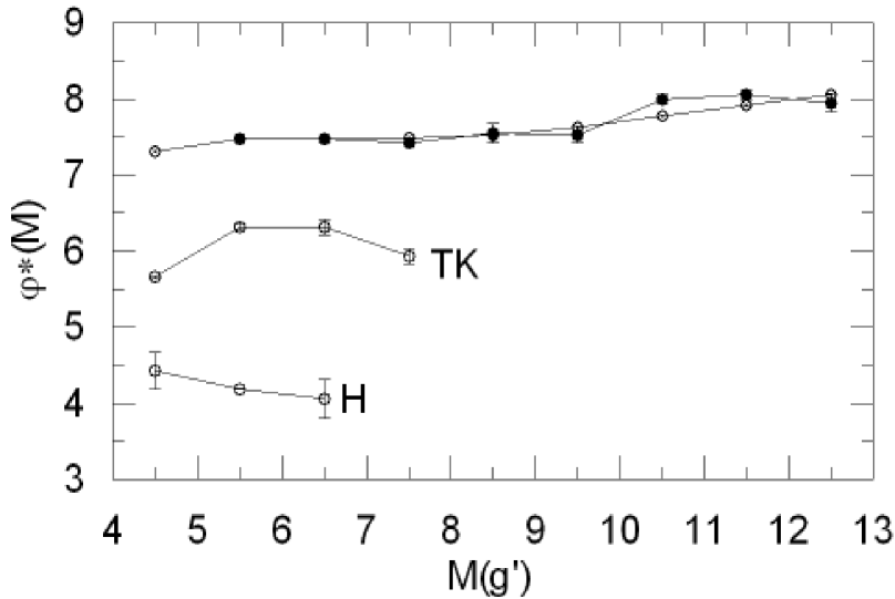
Figure 12: The local luminosity function obtained from combining the local space densities for the thin and thick discs and the halo, resulting from comparison of the derived space density function with the density laws, for different absolute magnitude intervals. The “$\odot$” symbols show the $Hipparcos$ values. TK and H corresponds to only thick disc and halo local luminosity, respectively.

5.2 Model parameter estimation by simultaneous comparison to the Galactic stellar populations

We estimated the model parameters for three populations simultaneously by comparison of the combined derived space density functions with the combined density laws. We carried out this work for two sets of absolute magnitude intervals, $4<M(g^{{}^{\prime}})\leq 10$ and $4<M(g^{{}^{\prime}})\leq 13$. The fit for the second interval was done due to our experience that model parameters are absolute magnitude dependent and that it covers the thin-disc stars with $10<M(g^{{}^{\prime}})\leq 13$, the density functions of which behave differently from the density functions for stars with other absolute magnitudes. Actually, we will see in the following that the luminosity function for the absolute magnitude interval $4<M(g^{{}^{\prime}})\leq 13$ differs from the one for stars with $4<M(g^{{}^{\prime}})\leq 10$ considerably (Fig. 14 and Fig. 16). The number of stars as a function of distance $r$ relative to the Sun for nine absolute magnitude intervals are given in Table 10 and the density functions per unit absolute magnitude interval evaluated by these data are shown in Tables 11 and 12 for the intervals $4<M(g^{{}^{\prime}})\leq 10$ and $4<M(g^{{}^{\prime}})\leq 13$ respectively.

Table 10: Number of stars as a function of distance $r$ relative to the Sun for nine absolute magnitude intervals (distances in kpc). Horizontal thick lines correspond the limiting distance of completeness.

$M(g^{{}^{\prime}})\rightarrow$	(4,5]	(5,6]	(6,7]	(7,8]	(8,9]	(9,10]	(10,11]	(11,12]	(12,13]
$r_{1}-r_{2}$	N	N	N	N	N	N	N	N	N
0.0-0.2								11	19
0.2-0.4						22	165	208	84
0.4-0.7				4	67	177	412	289	13
0.7-1.0				65	252	130	280	20
1.0-1.5			94	200	297	193	68
1.5-2.0		99	268	186	214	38
2.0-2.5		231	218	156	117
2.5-3.0	12	247	145	117	52
3.0-4.0	55	368	319	143
4.0-5.0	46	234	192	36
5.0-7.5	102	319	215
7.5-10.0	124	156	7
10.0-12.5	146	34
12.5-15.0	85
15.0-17.5	41
Total	611	1688	1458	907	999	560	925	528	116

5.2.1 Model parameters by means of absolute magnitudes $4<M(g^{{}^{\prime}})\leq 10$

The combined derived densities per absolute magnitude interval for three populations, the thin and thick discs and the halo for stars with $4<M(g^{{}^{\prime}})\leq 10$ (Table 11), are compared with the combined density laws (Fig. 13). The derived parameters are given in Table 13. All these parameters are in agreement with the ones given in Table 1, and they lie between two corresponding parameters cited in Section 5.1, except the scaleheight of thick disc, 760 pc, which is rather smaller than the scaleheight 839 pc, the smallest one in Table 7. Thus, the scaleheight 269 pc for the thin disc is between the ones for absolute magnitude intervals $10<M(g^{{}^{\prime}})\leq 11$ and $11<M(g^{{}^{\prime}})\leq 12$, and the logarithmic local space density 7.51 is almost equal to the corresponding one for the absolute magnitude interval $9<M(g^{{}^{\prime}})\leq 10$. For the thick disc, the local space density relative to thin disc, 6.46 per cent, is between the local space densities for the absolute magnitude intervals $6<M(g^{{}^{\prime}})\leq 7$ and $7<M(g^{{}^{\prime}})\leq 8$. It is interesting that the local space density for the halo relative to thin disc, 0.08 per cent, is almost equal to the one for the absolute magnitude interval $5<M(g^{{}^{\prime}})\leq 6$ in Table 8, however, the axial ratio $\kappa=0.55$ is considerably smaller than the ones in the same table. The resulting luminosity function (Fig. 14) from the comparison of the model with these parameters and the combined derived density functions per absolute magnitude interval is in agreement with the one of $Hipparcos$ (Jahreiss & Wielen 1997). However, the error bars are longer than the ones in Fig. 12, particularly for the faint magnitudes.

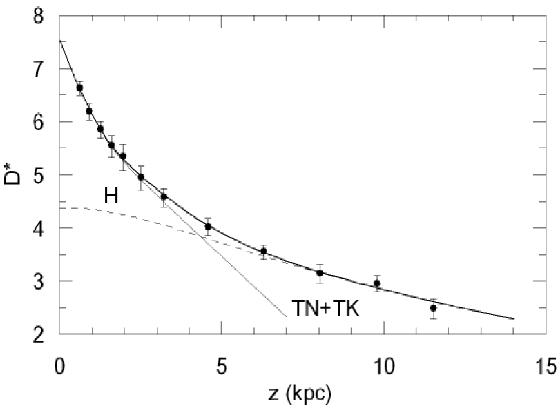
Figure 13: Comparison of the derived and combined space density function for the thin and thick discs and the halo with the combined density law, for stars with $4<M(g^{{}^{\prime}})\leq 10$.

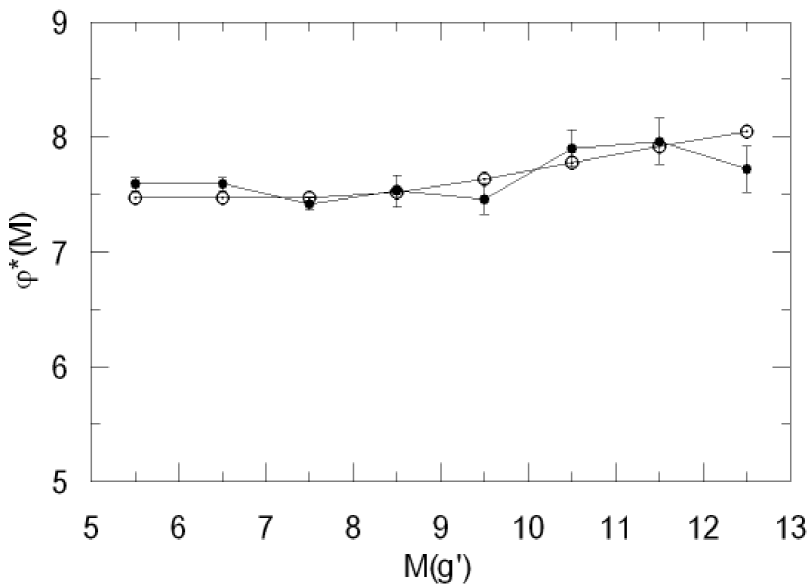
Figure 14: The local luminosity function resulting from the comparison of the combined derived space density function with the combined density law, for stars with $4<M(g^{{}^{\prime}})\leq 10$.

Table 11: The logarithmic space density function, $D^{*}=\log D+10$, per unit absolute magnitude interval for stars with $4<M(g^{{}^{\prime}})\leq 10$. $<N>$ is the mean of number of stars weighted by their numbers. The data are taken from Table 10. The other symbols are explained in the text (distances in kpc, volumes in pc³).

$r_{1}-r_{2}$	$\Delta V_{1,2}$	$r^{*}$	$z^{*}$	$<N>$	$D^{*}$
0.7-1.0	4.38 (5)	0.88	0.62	191	6.64
1.0-1.5	1.58 (6)	1.30	0.92	249	6.20
1.5-2.0	3.09 (6)	1.78	1.26	223	5.86
2.0-2.5	5.09 (6)	2.28	1.61	181	5.55
2.5-3.0	7.59 (6)	2.77	1.96	170	5.35
3.0-4.0	2.47 (7)	3.57	2.52	221	4.95
4.0-5.0	4.07 (7)	4.56	3.22	157	4.59
5.0-7.5	1.98 (8)	6.49	4.58	212	4.03
7.5-10.0	3.86 (8)	8.92	6.30	140	3.56
10.0-12.5	6.36 (8)	11.39	8.04	90	3.15
12.5-15.0	9.49 (8)	13.86	9.78	85	2.95
15.0-17.5	1.32 (9)	16.35	11.54	41	2.49

Table 12: The logarithmic space density function, $D^{*}=\log D+10$, per unit absolute magnitude interval for stars with $4<M(g^{{}^{\prime}})\leq 13$ (symbols as in Table 11).

$r_{1}-r_{2}$	$\Delta V_{1,2}$	$r^{*}$	$z^{*}$	$<N>$	$D^{*}$
0.2-0.4	3.74 (4)	0.33	0.23	152	7.61
0.4-0.7	1.86 (5)	0.59	0.42	293	7.20
0.7-1.0	4.38 (5)	0.88	0.62	221	6.70
1.0-1.5	1.58 (6)	1.30	0.92	230	6.16
1.5-2.0	3.09 (6)	1.78	1.26	223	5.86
2.0-2.5	5.09 (6)	2.28	1.61	180	5.55
2.5-3.0	7.59 (6)	2.77	1.96	170	5.35
3.0-4.0	2.47 (7)	3.57	2.52	277	5.05
4.0-5.0	4.07 (7)	4.56	3.22	213	4.72
5.0-7.5	1.98 (8)	6.49	4.58	212	4.03
7.5-10.0	3.86 (8)	8.92	6.30	140	3.56
10.0-12.5	6.36 (8)	11.39	8.04	90	3.15
12.5-15.0	9.49 (8)	13.86	9.78	85	2.95
15.0-17.5	1.32 (9)	16.35	11.54	41	2.49

Table 13: Galactic model parameters estimated by comparison of the logarithmic space density function for stars with $4<M(g^{{}^{\prime}})\leq 10$ (given in Table 11) and the combined density laws (Fig. 13). Symbols: $n^{*}$ is the logarithmic space density, $H$ is the scaleheight, $n/n_{1}$ is the local space density relative to the thin disc and $\kappa$ is the axial ratio for the halo.

Parameter	Thin disc	Thick disc	Halo
$n^{*}$	$7.51^{+0.04}_{-0.03}$	$6.32^{+0.06}_{-0.07}$	$4.41^{+0.38}_{-0.70}$
$H$ (pc)	$269^{+8}_{-8}$	$760^{+62}_{-55}$	$-$
$n/n_{1}$ (per cent)	$-$	$6.46$	$0.08$
$\kappa$	$-$	$-$	$0.55^{+0.25}_{-0.15}$

Table 14: Galactic model parameters estimated by comparison of the logarithmic space density function for stars with $4<M(g^{{}^{\prime}})\leq 13$ (given in Table 12) and the combined density laws (Fig. 14). Symbols are as in Table 13.

Parameter	Thin disc	Thick disc	Halo
$n^{*}$	$8.18^{+0.01}_{-0.01}$	$6.36^{+0.08}_{-0.08}$	$4.41^{+0.56}_{-0.90}$
$H$ (pc)	$173^{+3}_{-3}$	$822^{+99}_{-85}$	$-$
$n/n_{1}$ (per cent)	$-$	$1.51$	$0.02$
$\kappa$	$-$	$-$	$0.55^{+0.25}_{-0.15}$

5.2.2 Model parameters by means of absolute magnitudes $4<M(g^{{}^{\prime}})\leq 13$

We carried out the work cited in previous paragraph for stars with a larger range of absolute magnitude, i.e. $4<M(g^{{}^{\prime}})\leq 13$. The derived density function is given in Table 12 and its comparison with the combined density law is shown in Fig. 15. Most of the derived parameters (Table 14), especially the local densities, are rather different than the ones cited in Section 5.1 and 5.2.1. The reason for this discrepancy is that stars with absolute magnitudes $10<M(g^{{}^{\prime}})\leq 13$ have relatively larger local space densities ($Hipparcos$; Jahreiss & Wielen 1997) and are closer to the Sun relative to stars brighter than $M(g^{{}^{\prime}})=10$, and they affect the combined density function considerably. Also the corresponding luminosity function is not in agreement with the one of $Hipparcos$ (Fig. 16).

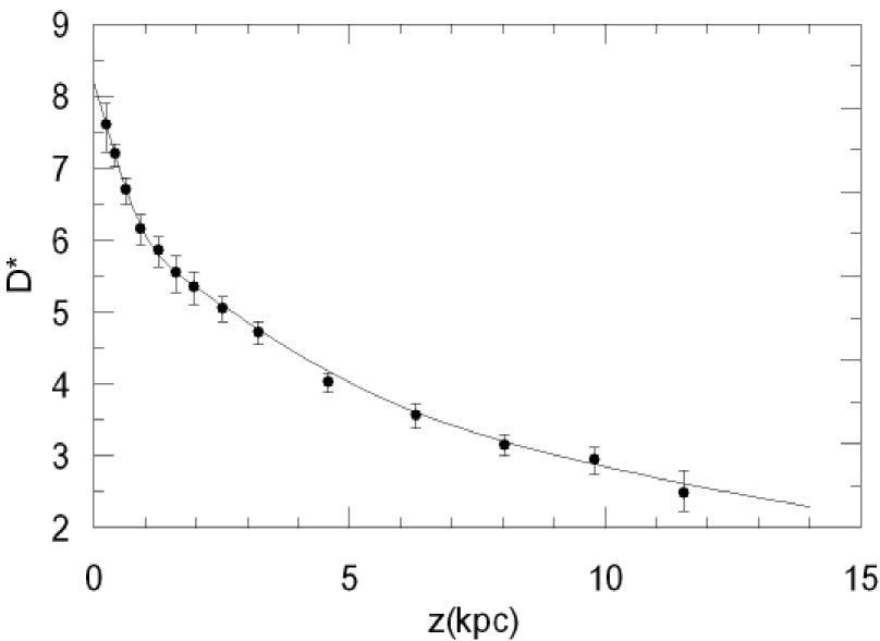
Figure 15: Comparison of the derived and combined space density function for the thin and thick discs and the halo with the combined density laws, for stars with $4<M(g^{{}^{\prime}})\leq 13$.

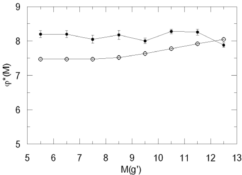
Figure 16: The local luminosity function resulting from the comparison of the combined derived space density function with the combined density law, for stars with $4<M(g^{{}^{\prime}})\leq 13$.

6 Discussion

We estimated the Galactic model parameters by comparison of the derived space density functions per absolute magnitude interval, in the perpendicular direction to the Galactic plane, with a unique density law for each population individually for the ELAIS field ($\alpha=16^{h}10^{m}00^{s},\delta=+54^{o}30^{{}^{\prime}}00{{}^{\prime\prime}}$; $l=84^{o}.27$, $b=+44^{o}.90$; 6.571 deg²; epoch 2000), by Vega photometry. The separation of stars into different populations has been carried out by their spatial position as a function of both absolute and apparent magnitude (KBH, see also Karaali 1994). This work covers nine absolute magnitude intervals, i.e. $4<M(g^{{}^{\prime}})\leq 5$, $5<M(g^{{}^{\prime}})\leq 6$, $6<M(g^{{}^{\prime}})\leq 7$, $7<M(g^{{}^{\prime}})\leq 8$, $8<M(g^{{}^{\prime}})\leq 9$, $9<M(g^{{}^{\prime}})\leq 10$, $10<M(g^{{}^{\prime}})\leq 11$, $11<M(g^{{}^{\prime}})\leq 12$ and $12<M(g^{{}^{\prime}})\leq 13$. However, the populations are not dominant in all absolute magnitude intervals. We consider two density laws for the thin-disc stars: the density law sech² fits better with the derived space density functions for the absolute magnitude intervals $10<M(g^{{}^{\prime}})\leq 11$ and $11<M(g^{{}^{\prime}})\leq 12$, whereas for the absolute magnitude intervals $5<M(g^{{}^{\prime}})\leq 6$, $6<M(g^{{}^{\prime}})\leq 7$, $7<M(g^{{}^{\prime}})\leq 8$ and $8<M(g^{{}^{\prime}})\leq 9$ the exponential density law is favorable as in our previous paper (KBH). Contrary to our expectation, for the absolutely faintest interval $12<M(g^{{}^{\prime}})\leq 13$ the exponential law (not the sech² one) fits better with the derived space density functions. $9<M(g^{{}^{\prime}})\leq 10$ is a transition absolute magnitude interval where sech fits better, a density law which does not correspond to anything physical. The scaleheight for the thin disc increases monotonically from 163 to 363 pc, when one goes from the absolute magnitude interval $12<M(g^{{}^{\prime}})\leq 13$ to $5<M(g^{{}^{\prime}})\leq 6$ with the exception scaleheight H=211 pc for the transition interval $9<M(g^{{}^{\prime}})\leq 10$ which is less than the one for the interval $10<M(g^{{}^{\prime}})\leq 11$, i.e. H=295 pc. Some researchers restrict their works related with the Galactic model estimation to absolute magnitude. The recent work of Robin et al. (2003) who treated stars with $M(V)\leq 8$ can be given as an example. Thus, if we consider the range of the scaleheight only for stars with $4<M(g^{{}^{\prime}})\leq 10$ in our work, we notice that it almost overlaps with the range of the scaleheight defined by the minimum and maximum scaleheights given in Table 1, i.e. 200-350 pc (we did not take into account the upper limit for the thin disc of Robin & Crézé (1986), 475 pc). The local space density for the thin disc decreases monotonically within the uncertainties, from absolutely faint magnitude intervals to the bright ones, however, the gradient converges to zero at the bright intervals in agreement with the corresponding local densities of $Hipparcos$ (Jahreiss & Wielen 1997).

Table 15: Comparison of the most appropriate Galactic model parameters for two works: (SA 114) for our previous work (KBH) and (ELAIS) for the present work.

	Thin disc				Thick disc				Halo
$M(g^{{}^{\prime}})$	H (kpc)		($n^{*}_{1}$)		H (kpc)		$n_{2}/n_{1}$(per cent)		$\kappa$		$n_{3}/n_{1}$(per cent)
Field$\rightarrow$	SA 114	ELAIS	SA 114	ELAIS	SA114	ELAIS	SA114	ELAIS	SA 114	ELAIS	SA 114	ELAIS
(4,5]						0.84				0.6
(5,6]	0.34	0.36	7.4	7.4	0.88	0.84	9.5	7.6	0.6	0.7	0.15	0.06
(6,7]	0.33	0.35	7.4	7.4	0.90	0.85	9.8	7.4	0.7	0.8	0.05	0.04
(7,8]	0.31	0.32	7.5	7.4	0.81	0.87	6.5	3.3	0.8		0.02
(8,9]	0.29	0.31	7.5	7.6	0.97		5.2
(9,10]	0.26	0.21	7.6	7.5
(10,11]	0.30	0.30	8.0	8.0
(11,12]	0.19	0.26	8.6	8.0
(12,13]	0.17	0.16	8.1	8.0

The logarithmic space densities for the thick disc could be derived for the absolute magnitude intervals $4<M(g^{{}^{\prime}})\leq 5$, $5<M(g^{{}^{\prime}})\leq 6$, $6<M(g^{{}^{\prime}})\leq 7$ and $7<M(g^{{}^{\prime}})\leq 8$. The range for the scaleheight is rather small, 839-867 pc, and the scaleheight itself is flat within the quoted uncertainties. The scaleheight for the thick disc in our work is in good agreement with the scaleheight claimed by many authors (cf. Yamagata & Yoshii 1992, von Hippel & Bothun 1993, Buser et al. 1998; 1999). However, contrary to our expectation, the range of the scaleheight for the thick disc cited very recently is large: actually Chen et al. (2001) and Siegel et al. (2002) give 0.58-0.75 and 0.7-1.0 kpc respectively. Now, let us compare these ranges with the ones in Tables 13 and 14, where the Galactic model parameters estimated by simultaneous comparison to the Galactic stellar populations correspond to stars with $4<M(g^{{}^{\prime}})\leq 10$ and $4<M(g^{{}^{\prime}})\leq 13$ respectively. The range for the scaleheight of thick disc is 705-822 for Table 13 and 737-921 pc for Table 14. We can easily see that they are in good agreement, especially if we round our values, i.e. 0.7-0.9 kpc, they overlap with the ones of Siegel et al. (2002). We should remind that the absolute magnitudes of stars treated by Siegel et al. (2002) extend down to $M(R)=10.2$ which corresponds to $M(g^{{}^{\prime}})>10.2$ mag in the Vega photometry. This comparison encourage us to argue two points:

1. The absolutely faint stars cause large ranges in the estimation of Galactic model parameters;

2. Galactic model parameters are mass (and hence absolute magnitude) dependent as claimed in our previous paper (KBH). The local space density for the thick disc relative to thin disc increases from 3.31 to 7.59 per cent, from absolutely faint magnitude intervals to the bright ones. The large values correspond to absolute magnitude intervals where thick disc is dominant (Table 7, Fig. 8). Here we reveal another property: although the range of absolute magnitude for the thick disc stars, $4<M(g^{{}^{\prime}})\leq 8$, is not large, the local space density for the thick disc cover almost all the range cited in the literature (see Table 1) and the larger number of stars results the larger local space density. Hence, we can add another point; and

3. The largeness of the local space density for an absolute magnitude interval for a specific population is proportional to the dominance of that population in the interval considered. Therefore, if a population is dominant in an absolute magnitude interval, then the local space density for that population is large.

The logaritmic space density functions for the halo could be derived only for three absolute magnitude intervals, $4<M(g^{{}^{\prime}})\leq 5$, $5<M(g^{{}^{\prime}})\leq 6$ and $6<M(g^{{}^{\prime}})\leq 7$, and they are compared with the de Vauculeurs density law. The local space density relative to the thin disc $(n_{3}/n_{1})$ could not be given for the interval $4<M(g^{{}^{\prime}})\leq 5$, due to the lack of local space density for this interval for the thin disc. For the intervals $5<M(g^{{}^{\prime}})\leq 6$ and $6<M(g^{{}^{\prime}})\leq 7$, $n_{3}/n_{1}=0.06$ and $n_{3}/n_{1}=0.04$ respectively, consistent with the results of Buser et al. (1998, 1999) and KBH. The numerical values for the axial ratio $\kappa$ for two intervals are close to each other, i.e. $\kappa=0.73$ and $\kappa=0.78$ for $5<M(g^{{}^{\prime}})\leq 6$ and $6<M(g^{{}^{\prime}})\leq 7$ respectively, but a bit less for the interval $4<M(g^{{}^{\prime}})\leq 5$, $\kappa=0.60$, consistent with the previous ones within the uncertainties however. It is interesting that the axial ratio estimated by simultaneous comparison to the Galactic stellar populations for stars within $4<M(g^{{}^{\prime}})\leq 13$ is lesser, $\kappa=0.55$ (Tables 13 and 14) than the ones cited above. It seems that absolutely faint magnitudes where halo stars are very rare causes bad $\kappa$ estimation.

Finally, we compared the Galactic model parameters estimated in our previous work ($l=68^{o}.15$, $b=-48^{o}.38$) and in this work ($l=84^{o}.27$, $b=+44^{o}.90$) in Table 15. The results confirm the idea that the Galactic model parameters are mass (and hence absolute magnitude) dependent. There is a good agreement between two sets of data, however, we should note some points and keep in mind in the comparison with the results that would appear in future:

(a) Although the scaleheights for a specific absolute magnitude interval of thin disc for two fields are rather close to each other, the local space density for the interval $11<M(g^{{}^{\prime}})\leq 12$ is a bit larger for the field SA 114 ($n_{1}^{*}=8.6$) than the one for the ELAIS field ($n_{1}^{*}=8.0$). This slight discrepancy probably originates from the previous work because the corresponding total local space density does not agree with the $Hipparcos$ (Jahreiss & Wielen 1997) one either;

(b) Although the scaleheights estimated for the thick disc for two fields are rather close to each other, the local space density relative to the local space density of thin disc for the field SA 114 is larger than the one for ELAIS field; and

(c) The axial ratio, $\kappa$, for the halo for two fields are almost the same, whereas the local space density relative the local space density of the thin disc for the absolute magnitude interval $5<M(g^{{}^{\prime}})\leq 6$ for the field SA 114 is 2.5 times that of the corresponding one for ELAIS field.

References

- [1] Bahcall J.N., Soneira R.M., 1980, ApJS, 44, 73
- [2] Beers T.C., Sommer-Larsen J., 1995, ApJS, 96, 175
- [3] Bertin A., Arnouts S., 1996, A&AS, 117, 393
- [4] Buser R., Rong J., Karaali S., 1998, A&A, 331, 934
- [5] Buser R., Rong J., Karaali S., 1999, A&A, 348, 98
- [6] Carney B.W., Latham D.W., Laird J.B., 1990, AJ, 99, 572
- [7] Chen B. et al. (the SDSS Collaboration), 2001, ApJ, 553, 184
- [8] Cox A.N., ed., 2000, Allen’s astrophysical quantities, AIP Press, Springer, New York
- [9] de Vaucouleurs G., 1948, Ann. d’Astrophys., 11, 247
- [10] del Rio G., Fenkart R.P., 1987, A&AS, 68, 397
- [11] Du C., Zhou X., Ma J., Bing-Chih A., Yang Y., Li J., Wu H., Jiang Z., Chen J., 2003, A&A, 407, 541
- [12] Eggen O.J., Lynden-Bell D., Sandage A.R., 1962, ApJ, 136, 748
- [13] Fan X., 1999, AJ, 117, 2528
- [14] Fenkart R.P., Topaktaş L., Boydag S., Kandemir G., 1987, A&AS, 67, 245
- [15] Freeman K., Bland-Hawthorn J., 2002, ARA&A, 40, 487
- [16] Gilmore G., Reid N., 1983, MNRAS, 202, 1025
- [17] Gilmore G., 1984, MNRAS, 207, 223
- [18] Gilmore G., Wyse R.F.G., 1985, AJ, 90, 2015
- [19] Hesser J.E., Harris W.E., Vandenberg D.A., Allwright J.W.B., Shott P., Stetson P.B., 1987, PASP, 99, 739
- [20] Jahreiss H., Wielen R., 1997, in Battrick B., Perryman M.A.C., & Bernacca P.L., eds, HIPPARCOS - Venice ’97. ESA SP-402, Noordwijk, p. 675
- [21] Karaali S., 1994, A&AS, 106, 107
- [22] Karaali S., Bilir S., Hamzaoğlu E., 2004, MNRAS, 355, 307 (KBH)
- [23] Kuijken K., Gilmore G., 1989, MNRAS, 239, 605
- [24] Lang K.R., 1992, Astrophysical Data I, Planets and Stars, Springer-Verlag, Berlin
- [25] Larsen J.A., 1996, Ph. D. Thesis, Univ. Minnesota
- [26] McMahon R.G., Walton N.A., Irwin M.J., Lewis J.R., Bunclark P.S., Jones D.H., 2001, New Astron. Rev., 45, 97
- [27] Norris J.E., Bessell M.S., Pickles, A.J., 1985, ApJS, 58, 463
- [28] Norris J.E., 1986, ApJS, 61, 667
- [29] Norris J.E., Ryan S.G., 1991, ApJ, 380, 403
- [30] O’Connell D.J.K., ed. 1958. Stellar Populations. Amsterdam: North Holland Press. Oort J.H., 1958. In O’Connell, p. 419
- [31] Ojha D.K., Bienaymé O., Mohan V., Robin A.C., 1999, A&A, 351, 945
- [32] Phleps S., Meisenheimer K., Fuchs B., Wolf C., 2000, A&A, 356, 108
- [33] Reid N., Majewski S.R., 1993, ApJ, 409, 635
- [34] Richer H.B., Fahlman G.G., 1986, ApJ, 304, 273
- [35] Robin A., Crézé M., 1986, A&A, 157, 71
- [36] Robin A.C., Haywood M., Crézé M., Ojha D.K., Bienaymé O., 1996, A&A, 305, 125
- [37] Robin A.C., Reylé C., Crézé M., 2000, A&A, 359, 103
- [38] Robin A.C., Reylé C., Derriére S., Picaud S., 2003, A&A, 409, 523
- [39] Sandage A., Fouts G., 1987, AJ, 93, 74
- [40] Schlegel D.J., Finkbeiner D.P., Davis M., 1998, ApJ, 500, 525
- [41] Searle L., Zinn R., 1978, ApJ, 225, 357
- [42] Siegel M.H., Majewski S.R., Reid I.N., Thompson I.B., 2002, ApJ, 578, 151
- [43] Tritton K.P., Morton D.C., 1984, MNRAS, 209, 429
- [44] von Hippel T., Bothun G.D., 1993, ApJ, 407, 115
- [45] Wyse R.F.G., Gilmore G., 1986, AJ, 91, 855
- [46] Wyse R.F.G., Gilmore G., 1989, Comments Astrophys., 13, 135
- [47] Yamagata T., Yoshii Y., 1992, AJ, 103, 117
- [48] Young P.J., 1976, AJ, 81, 807
- [49] Yoshii Y., Saio H., 1979, PASJ, 31, 339
- [50] Yoshii Y., 1982, PASJ, 34, 365
- [51] Yoshii Y., Ishida K., Stobie R.S., 1987, AJ, 93, 323