The effect of minihaloes on cosmic reionization

Abstract

One of the most debated issues in the theoretical modeling of cosmic reionization is the impact of small-mass gravitationally-bound structures. We carry out the first numerical investigation of the role of such sterile ‘minihaloes’, which serve as self-shielding screens of ionizing photons. Minihaloes are too small to be properly resolved in current large-scale cosmological simulations, and thus we estimate their effects using a sub-grid model, considering two cases that bracket their effect within this framework. In the ‘extreme suppression’ case in which minihalo formation ceases once a region is partially ionized, their effect on cosmic reionization is modest, reducing the volume-averaged ionization fraction by an overall factor of less than 15%. In the other extreme, in which minihalo formation is never suppressed, they delay complete reionization as much as $\Delta z\sim 2,$ in rough agreement with the results from a previous semi-analytical study by the authors. Thus, depending on the details of the minihalo formation process, their effect on the overall progress of reionization can range from modest to significant, but the minihalo photon consumption is by itself insufficient to force an extended reionization epoch.

1 Introduction

The study of reionization has recently witnessed an explosion of observational results. Since the advent of the new century, more than 10 quasars with $z>5.7$ have been discovered (White et al., 2003; Fan, 2004), indicating a strong increment of the neutral Lyman-$\alpha$ optical depth (Gunn & Peterson, 1965, GP) with increasing redshift, often interpreted as the end of reionization. At the same time observations of Cosmic Microwave Background (CMB) anisotropies have constrained the total optical depth of CMB photons to Thomson scattering in the range $\tau_{e}=0.17\pm 0.04$, where the quoted uncertainty depends on the analysis technique employed (Kogut et al., 2003; Spergel et al., 2003). Independent of the details, this optical depth can be converted into a reionization redshift that is $\lower 2.15277pt\hbox{$\;\buildrel>\over{\sim}\;$}10$. These tests,together with other probes of the high-$z$ universe as, such as Ly$\alpha$ emission and Gamma Ray Bursts (see Ciardi & Ferrara 2005 and references therein), provide an invaluable set of observational information. But only measurements of the 21 cm line emission from the neutral intergalactic medium (IGM) and collapsed haloes will be able to map the temporal and spatial evolution of the process itself (e.g. Madau, Meiksin & Rees, 1997; Shaver et al., 1999; Tozzi et al., 2000; Iliev et al., 2002, 2003; Ciardi & Madau, 2003; Furlanetto, Sokasian & Hernquist, 2004).

Numerical simulations and semi-analytical studies have struggled to match this early reionization (for a review see Barkana & Loeb, 2001; Ciardi & Ferrara, 2005), which requires an enhanced ionizing photon emission at high redshift, while delaying complete overlap until $z\sim 6$. Some models have even included scenarios such as double reionization through very massive, metal-free stars at high redshift, and more normal stars at lower redshift (e.g. Cen, 2003; Wyithe & Loeb, 2003), or early partial reionization due to a decaying particle or X-ray photons, followed by later full-reionization by normal stars (e.g. Oh, 2001; Chen & Kamionkowski, 2004; Hansen & Haiman, 2004; Ricotti & Ostriker, 2004). More conservatively, Ciardi, Ferrara & White (2003, CFW hereafter) have shown that normal stars with a slightly top-heavy Initial Mass Function (IMF) could suffice to produce an early reionization epoch, in agreement with the observations of the Wilkinson Microwave Anisotropy Probe (WMAP) satellite (e.g. Kogut et al., 2003).

The basic conclusion one can draw from these models is that boosting the ionizing photon production to the level required for early reionization is not a problem. Nevertheless, some tension might arise when the models are combined with the results from the Gunn-Peterson effect, as the reionization history must be tuned to (i) produce a large optical depth (to comply with the WMAP constraint), and (ii) to complete reionization at a relatively low redshift $\sim 6$ (as suggested by the GP data). Note, however, that this tension might be simply an artifact of the limited statistics of QSO absorption lines at these high redshifts (e.g. Choudhury & Ferrara, 2005). A scenario satisfying the above requirements could be one in which cosmic reionization starts at very high redshift and then goes through a long phase of partial ionization lasting approximately up to $z\sim 6$.

Such a long-lasting phase might be caused by the presence of small-scale, gravitationally-bound structures (Iliev, Scannapieco & Shapiro, 2005, hereafter ISS). In hierarchical theories like the cold dark matter (CDM) model, the smallest structures are the first to collapse and virialize, and in order to form stars they must radiate their virial energy. However, in a purely atomic gas of primordial composition, radiative cooling is ineffective below $10^{4}$ K. At these temperatures molecular hydrogen is the main coolant. But H₂ is easily dissociated by UV photons in the Lyman-Werner bands between 11.2 and 13.6 eV, which are copiously produced by the first stars (e.g. Haiman, Rees, & Loeb, 1997; Ciardi et al., 2000). On the other hand, an early X-ray background could provide enough free electrons to promote H₂ formation. Although the relative strength of the above feedback effects is controversial, the positive feedback from X-rays would not be able to balance UV photodissociation in the smallest objects (e.g. Haiman, Abel & Rees, 2000; Glover & Brand, 2003). Thus, we can expect a population of sterile “minihaloes” (MHs), which serve as self-shielding screens of ionizing photons and increase the local effective recombination rate of the gas. This prolongs the partial reionization phase and delays the end of the reionization process.

When an intergalactic I-front encounters a minihalo during cosmic reionization, the minihalo traps the I-front, converting it from a supersonic, weak R-type front to a subsonic, D-type front, which photoevaporates the minihalo gas. The first detailed studies of this interaction, using numerical gas dynamics simulations with radiative transfer, were reported in Shapiro, Iliev & Raga (2004, hereafter, SIR) and Iliev, Shapiro, & Raga (2005, hereafter, ISR). Since the gas in MHs is much denser than in the surrounding IGM, the recombination rate during this process is similarly increased. Furthermore, MHs were so abundant during reionization that a sight-line between any two given ionizing sources would have passed through many of them. This means that MHs have the potential to trap intergalactic I-fronts before they overlapped, and suggests that they may have drastically increased the global consumption of ionizing photons during reionization (Haiman, Abel & Madau, 2000; Barkana & Loeb, 2002; Shapiro, 2001; Shapiro, Iliev, Raga & Martel, 2003; Shapiro, Iliev & Raga, 2004; Iliev, Shapiro, & Raga, 2005).

While approximate schemes to account for the effect of MHs on photon consumption during reionization had been previously proposed (e.g. Haiman, Abel & Madau, 2000; Barkana & Loeb, 2002), they did not have the advantage of incorporating the results of the detailed numerical simulations of ionization front-MH interactions reported in SIR and ISR. These last studies not only highlighted the importance of accounting for the gradual “peeling away” of neutral MH gas by ionization fronts, but also provided detailed fits to the total number of ionizing photons absorbed as a function of MH mass, source flux level, and redshift. These fits then serve as a sound foundation for more detailed analytical treatments (such as Iliev, Scannapieco & Shapiro, 2005) and numerical investigations, that is the subject taken up here.

In the semi-analytical treatment in ISS, the rate of expansion of the I-fronts around individual source halos is modified to include the effect of MHs. This was done by generalizing the I-front continuity jump condition from Shapiro and Giroux (1987) to include the consumption of extra ionizing photons by MHs, as computed in SIR and ISR. The time evolution of the total ionized volume fraction of the universe was then calculated by summing these time-varying ionized volumes created by each source, over the statistical distribution of source halos in the universe. It was found that MHs increased the number of ionizing photons required to complete reionization by as much as a factor of 2, delaying completion of reionization by a redshift interval $\Delta z\sim 2.$ The fact that the mass fraction collapsed into MHs grows over time, suggested that the extra photon consumption by MHs would be more efficient at slowing the advance of I-fronts at late times. Instead, we found that the spatial clustering around each ionizing source kept the density of MHs fairly constant, where they were actually encountered by the I-fronts. As a result, MHs decreased the availability of photons to ionize the IGM at all epochs, delaying reionization, without extending its duration sufficiently to reconcile the GP and WMAP constraints. However, a more significant effect in that direction was found when the rising value of the small-scale clumping factor of the IGM was also taken into account.

Here we focus on a complementary approach to this problem, in which the extra photon consumption by MHs is incorporated as a “subgrid” correction in a numerical simulation of reionization. We use N-body results to identify the ionizing sources and the evolving IGM gas density field, a semi-analytical approach to identify the local density of MHs, and numerical radiative transfer techniques to propagate the I-fronts in three dimensions. The advantage of the numerical treatment is that it is liberated from the assumptions of spherically-averaged I-front propagation and a reliance on analytical models for clustering and bias. The numerical treatment, for example, is better equipped to account for the effects of clustered sources, which can result in H II regions powered by multiple sources, either simultaneously or sequentially. On the other hand, the semi-analytical approach has the advantage that it is not limited by finite numerical resolution and dynamic range, while these issues are inherent in the numerical treatment. Our hope is that, by offering these two distinct approaches, we can gain confidence in their answers, to the extent that they agree, remain cautious, to the extent that they do not, and gain more insight into the important effects than either one affords, on its own.

The main goal of this paper is to assess if the photon consumption provided by MHs can result in a slow and gradual reionization, thus offering a natural explanation for the high value of $\tau_{e}$ and, at the same time, account for the late reionization epoch hinted by the GP opacity. The paper is organized as it follows. In § 2 and 3 we describe the simulations of cosmic reionization in the absence of MHs and the physics of MHs photoevaporation, respectively. In § 4 we discuss the implementation of photoevaporation physics in the simulation of reionization. In § 5 we present our results and in § 6 we summarize our conclusions.

2 Simulations of Cosmic Reionization

In this study we recompute the simulations of cosmic reionization described in Ciardi, Stoehr & White (2003, hereafter CSW) and CFW, now including the effect of unresolved MHs. In this Section we briefly summarize the main features of the simulations. We refer the reader to the above papers for more details.

The simulations, performed with the N-body code GADGET (Springel, Yoshida & White, 2001), follow the evolution of an “average” region of the Universe. The “re-simulation” technique (e.g. Tormen, Bouchet & White, 1997) has been used to follow at higher resolution the dark matter distribution within an approximately spherical region of diameter $\sim 50h^{-1}$ Mpc included in a much larger volume ($479h^{-1}$ Mpc on a side; Yoshida, Sheth & Diaferio, 2001). The position and mass of dark matter haloes were determined with a friends-of-friends algorithm, while gravitationally-bound substructures within the haloes were identified with SUBFIND (Springel et al., 2001) and were used to build the merging tree for haloes and subhaloes. The smallest resolved haloes (which start to form at $z\sim 19$) have masses of $M\sim{\rm few}\times 10^{9}$ M_⊙, and the galaxy population was modeled via the semi-analytic technique of Kauffmann et al. (1999). A catalogue of galaxies for each of the simulation outputs was obtained, containing for each galaxy, among other quantities, its position, mass and star-formation rate (see Stoehr, 2003).

Within the high-resolution spherical sub-region, a cube of comoving side $L=20h^{-1}$ Mpc was extracted to study the details of the reionization process, using the Monte Carlo radiative transfer code CRASH (Maselli, Ferrara & Ciardi, 2003; Ciardi et al., 2001, CFMR hereafter) to model the propagation of ionizing photons into the IGM.

The only inputs necessary for the calculation are the gas density field and ionization state, as well as the source position and emission properties, which are provided at each output of the galaxy formation simulation described above. In particular, the dark matter density distribution is tabulated on a mesh using a Triangular Shaped Cloud (TSC) interpolation (Hockney & Eastwood, 1981). Assuming that the gas distribution follows that of the dark matter, the gas density in each cell grid is set requiring that $\Omega_{b}=0.04$. A number $N_{c}=128^{3}$ of cells have been used. To reduce the computational cost of the radiative transfer calculation, all the sources inside a grid cell are grouped into a single source placed at the cell center. Mass and luminosity conservation are assured.

3 Minihalo Photoevaporation

In the simulations described in the previous Section, the smallest resolution element is a grid cell, $156\,h^{-1}$ kpc on a side. Minihaloes are thus well below the resolution of the N-body simulation, and there are up to thousands of them inside each cell. The aim of this paper then is to model the presence and photoevaporation of MHs as sub-grid physics.

According to ISR, the total number of ionizing photons absorbed per minihalo atom during photoevaporation can be expressed as a function of the minihalo mass, $M$, redshift, $z$, and level of external ionizing photon flux, $F$, as follows

$$\bar{\xi}_{\rm MH}(M,z,F_{0})=1+\phi_{1}(M_{7})\phi_{2}(z)\phi_{3}(F_{0}),$$ (1)

where $M_{7}=M/(10^{7}M_{\odot})$, and

$$F_{0}\equiv\frac{F}{\{10^{56}\,\rm s^{-1}/[4\pi(1\,{\rm Mpc})^{2}]\}}.$$ (2)

For sources with a $5\times 10^{4}$ K blackbody spectrum, typical for O-stars, $\phi_{1}(M)\equiv 4.4\,(M_{7}^{0.334+0.023\lg M_{7}})$, $\phi_{2}(z)\equiv\left({1+z}\right)/10$ and $\phi_{3}(F_{0})\equiv F_{0}^{0.199-0.042{\rm lg}F_{0}}$. By combining equation (1) with the average number of minihaloes in a given volume, we can compute statistically the average ionizing photon consumption by minihaloes per total atom in this volume as

$$\bar{\xi}\equiv\frac{1}{\bar{\rho}_{m}}\int_{M_{\rm min}}^{M_{\rm max}}dM\,\frac{dn(M,z,\delta)}{dM}\,M\,\xi(M,z,F_{0}),$$ (3)

where $\bar{\rho}_{m}$ is the mean cosmological mass density and $dn(M,z,\delta)/dM$ is the number density of minihaloes in a region with an overdensity $\delta=\rho_{m}/{\bar{\rho}_{m}}-1$. Here the upper mass limit is set by the requirement that MHs are not able to cool atomically, that is $T_{\rm vir,max}=10^{4}$K or $M_{\rm max}=2.8\times 10^{9}(1+z)^{-3/2}M_{\odot}$ in our cosmology. Similarly, the lower mass limit, $M_{\rm min}$, is taken to be the (instantaneous) Jeans mass in the cold neutral medium. Note that we neglect the finite time delay for the gas to respond hydrodynamically to cooling (Gnedin & Hui, 1996). Accounting for this effect would raise the effective “filtering scale” in neutral regions, decreasing the impact of minihalos somewhat.

Adopting an extended PS approach (Lacey & Cole, 1993), we approximate the biased number density of minihaloes, $dn(M,z,\delta)/dM$, as

$$\frac{dn}{dM}=\frac{\bar{\rho}_{m}}{M}\left|\frac{d\sigma^{2}(M)}{dM}\right|f\left[1.68D^{-1}(z)-\delta_{L}(\delta),\sigma^{2}(M)\right],$$ (4)

where $D(z)$ is the linear growth factor at a redshift $z$, $\sigma^{2}(M)$ is the variance of linear fluctuations within a sphere containing a mass $M$, and

$$f(\delta_{L},\sigma^{2})\equiv\frac{\delta_{L}}{\sqrt{2\pi}\sigma^{3}}\exp\left(-\frac{\delta_{L}^{2}}{2\sigma^{2}}\right).$$ (5)

Finally, $\delta_{L}(\delta)$ is the linear overdensity corresponding to a nonlinear overdensity of $\delta$. If $\delta\geq 0$ these quantities can be related by the standard top-hat collapse model in terms of a “collapse parameter” $\theta$ as:

$$\delta=\frac{9}{2}\frac{(\theta-{\rm sin}\,\theta)^{2}}{(1-{\rm cos}\,\theta)^{3}}-1,$$ (6)

and

$$\delta_{L}=\frac{3}{5}\left(\frac{3}{4}\right)^{2/3}(\theta-{\rm sin}\,\theta)^{2/3}.$$ (7)

In underdense regions, $\delta$ and $\delta_{L}$ can be related by the solution given by Heath (1977) (see also Friedmann & Piran, 2001):

$$\delta=\eta(\delta_{L})^{-3}-1,$$ (8)

where

$$\eta(\delta_{L})=-\frac{\delta_{L}}{3}+\exp[-0.01\,(4.73\delta_{L}^{2}+0.83\delta_{L}^{3}+0.10\delta_{L}^{4})],$$ (9)

is the ratio of the comoving size of a perturbation to its initial comoving size. Note that eq. (4) is a Lagrangian number density, which is normalized by the mean density $\bar{\rho}_{m}$ in eq. (3) rather than an Eulerian density, which would have been normalized by $(\delta+1)\bar{\rho}_{m}$ instead.

Using eqs. (4)-(9) we can then re-write equation (3) as

$$\bar{\xi}(z,\delta,F_{0})=f_{\rm coll,MH}(z,\delta)+\phi_{3}(F_{0})I(z,\delta),$$ (10)

where

$$f_{\rm coll,MH}(z,\delta)\equiv\frac{1}{\bar{\rho}_{m}}\int_{M_{\rm min}}^{M_{\rm max}}dM\frac{dn(M,z,\delta)}{dM}M,$$ (11)

is the collapsed mass fraction in minihaloes and

$$I(z,\delta)\equiv\frac{1}{\bar{\rho}_{m}}\int_{M_{\rm min}}^{M_{\rm max}}dM\frac{dn(M,z,\delta)}{dM}M\phi_{1}(M)\phi_{2}(z),$$ (12)

such that $\phi_{3}(F_{0})I(z,\delta)$ is the extra number of ionizing photons absorbed per minihalo hydrogen atom.

4 Reionization Simulations with Minihaloes

In this Section we discuss the implementation used to include the physics of the MHs (§ 3) into the simulation of cosmic reionization (§ 2). In general, the galaxy formation simulations and the radiative transfer calculations are performed as described in § 3 of CSW, and only some of the quantities are modified to include the mean contribution of MHs, as follows.

The gas density field provided by the galaxy formation simulations is split into a diffuse component (the IGM) and MHs, according to the fraction of gas collapsed into MHs, $f_{\rm coll,MH}$ (equation 11). That is, if $n_{\rm H}$ is the hydrogen number density in a given cell, only a fraction $n_{\rm H}(1-f_{\rm coll,MH})$ is assigned to the diffuse gas component. From $f_{\rm coll,MH}$ we can derive the total mass of MHs in the cell as:

$$M_{\rm MH}=\rho_{m}\Delta l^{3}f_{\rm coll,MH},$$ (13)

where $\rho_{m}$ is the gas density in the cell and $\Delta l$ is its linear physical dimension. For our reference simulation $f_{\rm coll,MH}(z,\delta)$ is calculated at $(z_{cr},\delta_{cr})$, corresponding to the first photon package crossing of the cell and never increased thereafter, i.e. once a cell has been crossed by photons and fully or partially ionized, no new MHs are allowed to subsequently form in the cell. In almost all cases, complete ionization of a given cell occurs within $10^{6}$ years of the initial illumination. We call this reference case ‘extreme suppression’ and it places a lower limit to the effect of minihaloes on reionization.

On the other extreme, we consider the case in which we allow MHs formation in partially ionized and recombined regions. In this case, $f_{\rm coll,MH}$ is updated at each time step and it never becomes zero (we call this the ‘no suppression’ case). This is meant to put an upper limit on the effect of MHs, but the formation of sterile MHs in highly ionized regions is not supported by any strong physical motivation. In any case, although the impact of feedback on the formation of primordial, small-mass objects has been investigated by several authors (e.g. Gnedin, 2000; Oh & Haiman, 2003; O’Shea et al., 2005) a consensus has not yet been reached. In fact, an early X-ray background would heat the IGM before ionization from softer photons occurs and may provide an entropy floor even stricter than our “no suppression” case. As the presence and effectiveness of this mechanism remains highly uncertain however (see e.g. Oh & Haiman, 2003; Kuhlen & Madau, 2005), we can cautiously consider our calculations as providing reasonable estimates of as upper and lower limits on the impact of MHs on cosmic reionization.

To estimate the fraction of ionizing photons absorbed by MHs, we evaluate the optical depth of a given cell due to minihaloes alone, $\tau_{\rm MH}$, as:

$$\tau_{\rm MH}=0.56\sigma(\nu)n_{\rm H}f_{\rm coll,MH}\Delta l.$$ (14)

Here $\sigma(\nu)$ is the photoionization cross section at a frequency $\nu$ and the factor $f=0.56$ accounts for the average photon path length through a cell (CFMR). The total optical depth of a cell includes the contribution of both the diffuse gas, $\tau_{\rm diff}$, and MHs, $\tau=\tau_{\rm diff}+\tau_{\rm MH}$, with:

$$\tau_{\rm diff}=0.56\sigma(\nu)n_{\rm HI}(1-f_{\rm coll,MH})\Delta l.$$ (15)

In each cell along the path of the photon packet, the value of the hydrogen ionization fraction is updated according to eq. (10) of CFMR. In this case, though, the number of photons deposited in the diffuse component of the cell is replaced by $N_{\gamma}{\rm exp}(-\tau_{\rm MH})$, to take into account the photons absorbed by the MHs. Here $N_{\gamma}$ is the number of photons contained in the monochromatic packet that illuminates the cell. Any photons in the package not absorbed by either the diffuse gas or the MHs in the cell are passed onto the next cell.

To determine when the MHs in a given cell should be considered completely photoevaporated in the ‘extreme suppression’ case, we proceed as follows. If $(N_{\gamma,{\rm MH}})_{i}$ is the number of photons absorbed by MHs in a given cell at time step $i$ of the simulation, the fraction of MHs mass that these photons photoevaporate is:

$$({\cal F}_{\rm MH,evap})_{i}=\frac{(N_{\gamma,{\rm MH}})_{i}}{n_{\rm H}\Delta l^{3}\bar{\xi}},$$ (16)

where $\bar{\xi}$ is given by equation (10). The mass evaporated from the minihaloes, $M_{\rm MH}{\cal F}_{\rm MH,evap}$, is transferred to the IGM and $f_{\rm coll,MH}$ is modified accordingly. Note that, as we assume that once the cell has been illuminated no new MHs form, at each step only the flux dependent coefficient in equation (10), $\phi_{3}(F_{0})$, is updated according to the value of the current flux reaching the cell, $F$, while the rest is kept constant at $(z_{cr},\delta_{cr})$. $F$ is given by:

$$F=\frac{N_{\gamma}}{4\pi d^{2}\Delta t},$$ (17)

where $\Delta t$ is the time elapsed since a photon packet has gone through the cell and $d$ is the distance from the source. Once the sum $\sum_{i}({\cal F}_{\rm MH,evap})_{i}$ becomes equal to unity, we set $f_{\rm coll,MH}=0$ and consider the minihaloes gone thereafter. Only the number of photons necessary to complete photoevaporation are absorbed during the final step in which this condition is met.

In the ‘no suppression’ case instead, formation of minihaloes can occur at any time. For this reason, all the quantities in equation (10) are always updated. In particular, at each time step, we first calculate how much new mass has gone in MHs and update $f_{\rm coll,MH}(z,\delta)$ accordingly. We then subtract the evaporated mass from the MHs and transfer it to the IGM. In this case, when the sum $\sum_{i}({\cal F}_{\rm MH,evap})_{i}$ becomes equal to unity, new MHs are still allowed to form.

Finally, a slightly different approach is used for MHs inside a computational cell containing an ionizing source (see Appendix).

5 Results

5.1 Reionization histories

We quantify the impact of MHs on the progress of cosmic reionization by computing the volume-averaged ionization fraction, $x_{v}$, as a function of redshift, as shown in Figure 1. In our reference run (open circles) we adopt an emission spectrum typical of metal-free stars, a mildly top-heavy Larson IMF with characteristic mass of 5 M_⊙ and an effective escape fraction of ionizing photons $f_{esc}=20$%.

From a comparison with the analogous run in the absence of MHs (triangles; L20, ‘early’ reionization case in CFW), it is clear that the presence of MHs reduces the average ionization fraction most at early times, where the difference is $\approx$ 15%, while at later times the difference is $\;\buildrel<\over{\sim}\;$ 10%. This reflects the fact that less than 20% of the emitted photons in our model are absorbed by MHs at high redshifts, and this fraction decreases with decreasing redshift. Of the above percentage only $\;\buildrel<\over{\sim}\;$ 5% is absorbed by MHs in the source cells. This is mainly because there are only $\sim 150$ (4000) source cells at $z\sim 19$ (10), while there are about $2\times 10^{6}$ cells in the simulation. In both cases reionization is complete by $z_{ion}\sim 13$.

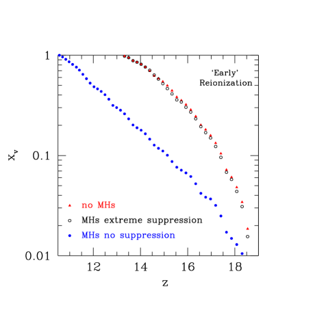
Figure 1: Evolution of the volume-averaged ionization fraction for three different simulation runs (see text for details): run with no MHs (triangles), run with MHs and ‘extreme suppression’ of their formation (open circles), and run with MHs and ‘no suppression’ of their formation (filled circles). Results are for an ‘early’ reionization case.

In Figure 2 we show the evolution of the MH collapsed fraction (ignoring photoevaporation, dotted line, open circles) and the fraction of photoevaporated MH mass (dashed line, open circles). The MHs collapsed fraction increases with decreasing redshift, until it reaches a plateau, corresponding to the epoch at which all the cells in the simulation have been crossed by photons and no more MH formation is allowed. Note that the total mass in the simulation box should be constant, but small fluctuations are possible as it is cut from a spherical region that is embedded in a much larger volume. The fraction of photoevaporated mass of MHs increases with time, until a value of the order of unity is reached at $z\sim 14$. Note that reionization of the IGM and complete MHs photoevaporation do not necessarily coincide, as there could be cells in which the ionization fraction of the diffuse gas is $\sim 1$, but some MHs still survive photoevaporation, or vice-versa.

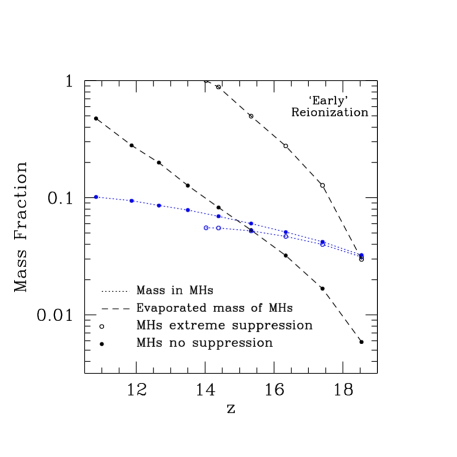
Figure 2: Redshift evolution of the fraction of total mass that is in MHs (excluding photoevaporation, dotted lines) and the fraction of mass in MHs which is photoevaporated (dashed lines). Filled (open) circles indicate a case of ‘no suppression’ (‘extreme suppression’) of MHs formation. Results are for an ‘early’ reionization case.

The ‘no suppression’ case (filled circles in Fig. 1) shows a much stronger effect due to MHs, which absorb 80-90% of the ionizing photons. As a result, reionization is delayed by $\Delta z\sim 2$. These results are similar to those obtained in ISS, which was largely focused on the impact of MH around individual sources, which were later summed together to give a rough estimate of the total MH impact on reionization. This means that each source in ISS saw a full compliment of MH, a picture very much like the ‘no suppression’ case studied here.

In Figure 2 the fraction of mass in MHs (dotted line, filled circles) follows a trend similar to the ‘extreme suppression case’, but now the abundance of MHs increases at late times, and at early times the fractional abundance of MHs is slightly higher. At all redshifts, the fraction of mass in MHs that is photoevaporated (dashed line, filled circles) is much smaller and increases more slowly than the ‘extreme suppression’ case. This is because MHs are continuously re-formed, while in the previous case no re-formation follows the almost instantaneous photoevaporation. As a consequence of re-formation, MHs survive also after complete reionization of the diffuse gas. If this is the case, their presence would still be visible in terms of, e.g., a contribution to the optical depth to ionizing photons and to the 21 cm emission line.

Finally, we have also explored the ‘late’ (S5) reionization case of CFW, in which a Salpeter IMF and $f_{esc}=5$% are adopted. Carrying out an ‘extreme suppression’ simulation, we find that the effect of MHs is qualitatively and quantitatively similar to our ‘early’ reionization model in which no MH reformation was allowed. Less than 20% of photons are absorbed by MHs at any redshift. This may reflect the fact that our MH collapsed fraction did not increase much with decreasing redshift above the level obtained at the higher redshifts of our early reionization case plotted in Figure 2. Here we note that the MH collapsed fraction is somewhat lower for this study than it was in ISS, due to our choice of the unknown small-scale power spectrum and, to a lesser extent, our coarse-grain density field. We discuss their impact on our results in Sec. 5.3.

5.2 Thomson Scattering Optical Depth

From the above reionization histories it is possible to derive the expected optical depth to electron scattering, $\tau_{e}$, as:

$$\tau_{e}(z)=\int_{0}^{z}\sigma_{T}n_{e}(z^{\prime})c\left|\frac{dt}{dz^{\prime}}\right|dz^{\prime},$$ (18)

where $\sigma_{T}=6.65\times 10^{-25}$ cm² is the Thomson cross section and $n_{e}(z^{\prime})$ is the mean electron number density at $z^{\prime}$. Prior to complete reionization, $n_{e}$ is obtained from the simulations at each redshift as $n_{e}=\sum_{i}^{N_{c}}x_{i}n_{i}(1-f_{\rm coll,MH})/N_{c}$, where the sum is performed over all the cells and $x_{i}$ is the ionization fraction in cell $i$. Once reionization is completed, we simply assume complete hydrogen and He I ionization throughout the box. We also assume complete He II reionization after $z=3$. We find that the Thomson scattering optical depth is $\tau_{e}=0.16$ for the ‘early’ reionization case without MH reformation, $\tau_{e}=0.12$ for the ’early’ case in which re-formation is allowed, and $\tau_{e}=0.10$ for the ‘late’ case without re-formation.

5.3 Model Uncertainties

In this Section we discuss the approximations and assumptions we adopted to model the effect of MHs on the progress of reionization.

The MH photoevaporation simulations by ISR on which we based our model span a range of fluxes $0.01<F_{0}<1000$. Very close to the ionizing sources, however, the normalized photon flux $F_{0}$ in equation (17) can exceed 1000. In the framework of our galaxy model this occurs rarely, in less than 2% of the cases, and thus it affects only a small fraction of the volume of the simulation. In such cases we set $F_{0}=1000$ in equation (1), which is a reasonable approximation since at high fluxes the MHs photon consumption dependence on the external flux becomes relatively weak. However, under different assumptions about the sources lifetimes, e.g. short-lived sources, the photon consumption by minihaloes would be higher. In a higher percentage of cases ($\sim 10$%), $F_{0}$ becomes smaller than 0.01. When the flux becomes so low, relatively few additional photons per atom are needed to evaporate the MHs and thus we assume that just one photon per atom is absorbed if $F_{0}\leq 0.01$. Both of these approximations are small, but conservative in terms of estimating the photon consumption by MHs.

For each output of the N-body simulations, the dark matter density distribution (and consequently the gas distribution, which is assumed to follow that of the dark matter) is tabulated on a mesh using a TSC interpolation (Hockney & Eastwood, 1981). The TSC interpolation has the advantage of producing smoothed density values at the positions of the grid cells, as required for the radiative transfer computation. However it is not adaptive and density variations on sub-grid scales are thus smoothed out, reducing the contrast of the dark matter density distribution. In CSW this effect is discussed in terms of a comparison between the TSC interpolation and a 32-particle SPH kernel, which should better capture the density contrasts. They found that the overall agreement for low and intermediate density is reasonable, but the smoothing of the TSC scheme is clearly visible at high densities, especially at the lower redshifts (Fig. 9 of CSW). This can lead to an underestimate of the value of $\delta$ at $z\lower 2.15277pt\hbox{$\;\buildrel<\over{\sim}\;$}12$ and dark matter densities $\rho\lower 2.15277pt\hbox{$\;\buildrel>\over{\sim}\;$}10^{-(3-4)}$ M${}_{\odot}/h({\rm kpc}/h)^{-3}$, depending on $z$. To estimate the error introduced by the TSC scheme, we computed the ratio of the average number of extra photons absorbed per unit hydrogen atom at $z=10$ in both the TSC and SPH scheme. This is

$$\frac{\sum_{i}^{N}\phi_{3}(F_{0,i}^{\rm TSC}){{\bar{\rho}}_{m}}(10)I(10,\delta^{\rm TSC}_{i})}{\sum_{j}^{N}\phi_{3}(F_{0,i}^{\rm SPH}){{\bar{\rho}}_{m}}(10)I(10,\delta^{\rm SPH}_{i})}.$$ (19)

In general, $\phi_{3}(F_{0,i}^{\rm TSC})$ and $\phi_{3}(F_{0,i}^{\rm SPH})$ need not be equal and will depend in detail on the formation and propagation of the ionization fronts in the simulations. However, as a rough estimate we simply factor out these terms, leaving a ratio of 1.030, or an error of $\sim$ 3% due to smoothing.

Due to our coarse-grained density field the total minihalo collapsed fraction in our computational volume obtained using our model (Fig. 2) is slightly lower than the global collapsed fraction obtained directly from analytical estimates (e.g. using PS or ST mass functions), particularly at later times when density fluctuations become more nonlinear. Higher-resolution N-body simulations would be required to better calibrate the mass function-local overdensity relationship better, but this goes beyond the scope of this paper. Note that these effects are most severe in cells containing ionizing sources, in which internal density contrasts are higher.

The semi-analytical treatment by ISS found that the importance of MHs as consumers of ionizing photons was higher if each source emitted its total lifetime supply of ionizing photons in a short burst at higher luminosity than if it emitted the same number of photons continuously over time at lower luminosity. In the Monte-Carlo reionization simulations reported here, each source is assumed to release its supply of ionizing photons spread out over the time between time-slices of the density field which were provided by the galaxy formation simulations. This results in longer source lifetimes and smaller luminosities than the fiducial case considered by ISS, involving short-lived sources. It is possible, therefore, that the MH correction effect would have been higher if we had, instead, assumed shorter source lifetimes.

As there are currently no direct constraints on the power spectrum of density fluctuations at minihalo scales, our estimates require a large, uncertain extrapolation. Although the transfer function we adopted is consistent with the simulations, assuming a different transfer function, such as the often-used one by Eisenstein & Hu (1999), can change the minihalo numbers significantly. For this particular application, the collapsed fraction in minihaloes for the Eisenstein & Hu (1999) power spectrum is larger than our fiducial model by almost a factor of two, implying a similar correction factor to the global effect of minihaloes. In fact, we have conducted a comparison simulation for the ‘extreme suppression’ case in which we use the Eisenstein & Hu (1999) power spectrum for the minihalo component, and we obtain an ionization fraction which is $\sim$ 90% of our fiducial run. Since currently there are no observational constraints to distinguish one of these transfer functions from the other, we have chosen to remain consistent with our large-scale N-body simulations, but again, this could result in a conservative estimate of the minihalo photon consumption during reionization.

A similar uncertainty arises from our choice of an analytic form for the MH mass function. Over the relevant redshifts, shifting from the Press-Schechter mass function to a Sheth & Tormen (2002) form would decrease the total mass in minihalos by roughly a factor of 1.5. However, there is little evidence to motivate the use of this more complicated expression at very high redshifts. In fact, the few simulations of high-z small-scale structure formation that exist seem to agree reasonably well with the Press-Schechter approach (Shapiro, 2001; Jang-Condell & Hernquist, 2001; Cen et al., 2004).

The resolution of the simulations is not able to capture the IGM density distribution on very small scales. Usually this is taken into account, both in numerical simulations and semi-analytic approaches, through the so called gas clumping factor. As the main goal of this study is to discuss the effect of MHs on the reionization process through a direct comparison with the simulations described in CSW and CFW, we have not included this effect. Its inclusion would delay the reionization process of an amount depending on the adopted value or expression for the clumping factor (see e.g. ISS). It should be noted, however, that according to the results of ISS, any increase of the global photon consumption due to minihaloes is combined with the increased consumption due to recombinations in the clumpy IGM, often amplifying their impact. Any complete treatment of the effect of small-scale structures reionization should therefore include both effects.

6 Conclusions

We have investigated the impact of minihaloes on the reionization process by means of a combination of high-resolution N-body simulations (to describe the dark matter and diffuse gas evolution), high-resolution hydrodynamical simulations (to examine the photoevaporation of minihaloes), a semi-analytic model of minihalo formation (to follow their biased distribution), and the Monte Carlo radiative code CRASH (to follow the propagation of ionizing photons). We have studied the process assuming different parameters that regulate the ionizing photon emission and different prescriptions for the evolution of minihaloes. The main results discussed in this paper can be summarized as follows.

$\bullet$ If minihalo formation in a cell is completely suppressed once the first photon packet arrives at the cell, i.e. in partially or fully ionized cells (‘extreme suppression’ case), we find that their effect on cosmic reionization is modest, with a volume averaged ionization fraction that is only $\lower 2.15277pt\hbox{$\;\buildrel<\over{\sim}\;$}15\%$ lower than the one when minihaloes are ignored. Only less than 20% of the total emitted ionizing photons are absorbed by minihaloes at any redshift. Complete reionization is not delayed significantly by the presence of minihaloes.

$\bullet$ If minihalo formation is not suppressed (‘no suppression’ case), then up to 80-90% of the emitted ionizing photons are absorbed by MHs and complete overlap can be delayed by as much as $\Delta z\sim 2$.

The ‘no suppression’ case is in good agreement with the results of the semi-analytical approach described in ISS. However, we find that the impact of MHs is smaller than the estimates by Haiman, Abel & Madau (2000) and Barkana & Loeb (2002), as these authors have overestimated the number of photons required to photoevaporate a MH. In fact, Barkana & Loeb (2002) use static models of clouds in thermal and ionization equilibrium without accounting for gas dynamics. For this reason they fail to capture some essential physics and overestimate the number of recombinations inside MHs. Haiman, Abel & Madau (2000) employ hydrodynamic simulations to study photoevaporation, but they do not include radiative transfer. Shapiro, Iliev & Raga (2004) and Iliev, Shapiro, & Raga (2005) (on which our calculations are based) found that the effect of ignoring radiative transfer and its feedback on the gas dynamics is to significantly overestimate the number of ionizing photons required to evaporate a MH.

As discussed in § 5.3, there are still uncertainties in our model, some of which are conservative in terms of estimating the photon consumption per minihalo. However, the ‘no suppression’ case certainly provides a liberal overestimate of the MH number density, which is likely to more than balance these effects. On the other hand, the ‘extreme suppression’ case provides a lower limit to the average MH number density, since it assumes that no new MHs form in any cell that has ever been exposed to ionizing photons, no matter how weakly or long ago, and thus it is likely to bracket the MH correction effect from below. It is with some confidence, then, that we can limit the true impact of minihaloes to lie between the extreme cases considered here, although future investigations will be necessary to limit this range further. Thus, our results indicate that the photon sink provided by these structures is not sufficient by itself to force a long-lasting phase of partial IGM ionization. This agrees with the conclusion of ISS for the cases that neglected the small-scale clumping of the IGM. Thus the resolution of the apparent conflict between the high electron scattering optical depth in the WMAP data and the low reionization redshift inferred by QSO absorption line experiments should rely on additional processes, such as the evolving small-scale IGM gas clumping factor, feedback effects or a transition in the star formation mode.

Appendix A Minihaloes in source cells

To account for the presence of MHs in computational cells that contain ionizing sources, we must take a slightly different approach from that described in §4. The reason is that at high redshift the ionizing sources were rare peaks of the density distribution, and thus minihaloes were strongly clustered around them. To account better for this clustering, we calculate the total number of photons absorbed by the gas (both diffuse and MHs) in that cell, $N_{s}$, using a simplified version of the analytical model we developed previously in ISS. In the current simulations we group all sources within each cell into a single source with a mass equal to the sum of the individual masses. Note however that such multiple sources only occur at the latest redshifts simulated and thus this approximation has only a minor effect on our results.

From ISS, the rate of expansion of the comoving volume about an ionized source of mass $M_{s}$ is given by

$$\frac{dV_{I}}{dt}=\frac{\dot{N}_{\gamma}(n_{H}^{0})^{-1}-\alpha_{B}\,(1+z)^{3}\,n_{H}^{0}(V_{I}-V_{0})}{1-f_{\rm coll}(M_{s},r)+\bar{\xi}_{\rm src}(M_{s},z,F_{0})},$$ (20)

where $n_{H}^{0}$ is the average comoving number density of hydrogen, $\alpha_{B}=2.6\times 10^{-13}$ cm³ s^-1 is the case B recombination coefficient for hydrogen at $10^{4}$ K, $V_{0}$ is the comoving volume initially carved out by the material making up the sources, and

$$f_{\rm coll,MH,src}(M_{s},z,r)=\frac{1}{{\bar{\rho}}_{m}}{\int_{M_{\rm min}}^{M_{\rm max}}dM\,\frac{dn(M,z,r|M_{s})}{dM}\,M\,},$$ (21)

and

$$\bar{\xi}_{\rm src}(M_{s},z,F_{0},r) = \frac{1}{{\bar{\rho}}_{m}}\int_{M_{\rm min}}^{M_{\rm max}}dM\times$$

$$\qquad\frac{dn}{dM}(M,z,r|M_{s})\,M\,\xi(M,z,F_{0}),$$

are the MH collapse fraction and average number of extra absorbed photons by MHs at a Lagrangian distance $r$ from a source of mass $M_{s}$ at a redshift $z$ shining with a flux $F_{0}$. Both $f_{\rm coll}(M_{s},z,r)$ and $\bar{\xi}_{\rm src}(M_{s},z,F_{0},r)$ make use of the biased number density of minihaloes, forming at a distance $r$ from the source halo. To calculate this quantity, we make use of the analytical formalism described in detail in Scannapieco & Barkana (2002) (see also Porciani et al., 1998). Here the biased number density is given as

$$\frac{dn}{dM}(M,z,r|M_{s})=\frac{dn^{2}}{dMdM_{s}}(M,z,M_{s},z,r)\left[\frac{dn}{dM_{s}}(M_{s},z)\right]^{-1},$$ (23)

where $dn/dM_{s}$ is the usual PS mass function and $\frac{dn^{2}}{dMdM_{s}}(M,z,M_{s},z,r)$ is the bivariate mass function that gives the product of the differential number densities at two points separated by an initial comoving distance $r$, at any two masses and redshift. Note that this expression interpolates smoothly between all standard analytical limits, including those of Mo & White (1996) and Lacey & Cole (1993), and it has also been carefully validated against simulations (Scannapieco & Thacker, 2005).

Finally, we compute $N_{s}$ by integrating eq. (20) up until the time $t_{\rm cell}$ at which the total mass contained within the ionized region is equal to the mass contained within the source cell. The number of photons absorbed is then simply $N_{s}=t\dot{N}_{\gamma},$ which is imposed by adopting a lower effective escape fraction, such that the total number of ionizing photons leaving the source cell is decreased.

References

- Barkana & Loeb (2001) Barkana R., Loeb A., 2001, Phys. Rep., 349, 125
- Barkana & Loeb (2002) Barkana R. & Loeb A. 2002, ApJ, 578, 1
- Cen (2003) Cen R., 2003, ApJ, 591, 12
- Cen et al. (2004) Cen, R., Dong, F., Bode, P., & Ostriker, J. P. 2004, ApJ, submitted (astro-ph/0403352)
- Chen & Kamionkowski (2004) Chen X., Kamionkowski M., 2004, Phys. Rev. D, 70, 3502
- Choudhury & Ferrara (2005) Choudhury T. R., Ferrara A., 2005, MNRAS, 361, 577
- Ciardi & Ferrara (2005) Ciardi B., Ferrara A., 2005, Space Science Reviews, 116, 625
- Ciardi et al. (2000) Ciardi B., Ferrara A., Governato F., & Jenkins A. 2000, MNRAS, 314, 611
- Ciardi et al. (2001) Ciardi B., Ferrara A., Marri S., Raimondo G., 2001, MNRAS, 324, 381 (CFMR)
- Ciardi, Ferrara & White (2003) Ciardi B., Ferrara A., White S. D. M., 2003, MNRAS, 344, L7 (CFW)
- Ciardi & Madau (2003) Ciardi B., Madau P., 2003, ApJ, 596, 1
- Ciardi, Stoehr & White (2003) Ciardi B., Stoehr F., White S. D. M., 2003, MNRAS, 343, 1101 (CSW)
- Efstathiou, Bond, & White (1992) Efstathiou, G., Bond, J. R. & White, S. D. M. 1992, MNRAS, 258, 1
- Eisenstein & Hu (1999) Eisenstein, D. J. & Hu, W. 1999, ApJ, 511, 5
- Fan (2004) Fan X., et al. , 2004, AJ, 128, 151
- Friedmann & Piran (2001) Friedmann, Y. & Piran, T. 2001, ApJ, 548, 1
- Furlanetto, Sokasian & Hernquist (2004) Furlanetto S. R., Sokasian A., Hernquist L., 2004, MNRAS, 347, 187
- Glover & Brand (2003) Glover S. C. O., Brand P. W. J. L., 2003, MNRAS, 340, 210
- Gnedin (2000) Gnedin N. Y., 2000, ApJ, 542, 535
- Gnedin & Hui (1996) Gnedin, N. Y. & Hui, L. 1996, MNRAS, 296, 44
- Gunn & Peterson (1965) Gunn J., Peterson B. A., 1965, ApJ, 142, 1633
- Haiman, Abel & Rees (2000) Haiman, Z., Abel, T., Rees M. J., 2000, ApJ, 534, 11
- Haiman, Abel & Madau (2000) Haiman, Z., Abel, T., & Madau, P. 2000, ApJ, 551, 599
- Haiman, Rees, & Loeb (1997) Haiman, Z., Rees, M., & Loeb, A. 1997, ApJ, 476, 458 (erratum 484, 985)
- Hansen & Haiman (2004) Hansen S., Haiman Z., 2004, ApJ, 600, 26
- Heath (1977) Heath, D. J. 1977, MNRAS, 179, 351
- Hockney & Eastwood (1981) Hockney R. W., Eastwood J. W., 1981, in ”Computer Simulations Using Particles”; New York: McGrow-Hill
- Iliev et al. (2002) Iliev I. T., Shapiro P. R., Ferrara, A., Martel, H. 2002, ApJ, 572, 123L
- Iliev et al. (2003) Iliev I. T., Scannapieco E., Martel, H., Shapiro P. R., 2003, MNRAS, 341, 81
- Iliev, Scannapieco & Shapiro (2005) Iliev I. T., Scannapieco E., Shapiro P. R., 2005, ApJ, 624, 491 (ISS)
- Iliev, Shapiro, & Raga (2005) Iliev I. T., Shapiro P. R., & Raga, A. C., 2005, MNRAS, 361, 405 (ISR)
- Jang-Condell & Hernquist (2001) Jang-Condell, H., & Hernquist, L. 2001, ApJ, 548, 68
- Kauffmann et al. (1999) Kauffmann G., Colberg, J. M., Diaferio A., White S. D. M., 1999, MNRAS, 303, 188
- Kuhlen & Madau (2005) Kuhlen M., Madau P., 2005, astro-ph/0506712
- Kogut et al. (2003) Kogut A. et al. , 2003, ApJS, 148, 161
- Lacey & Cole (1993) Lacey, C. & Cole, S. 1993, MNRAS, 262, 627
- Madau, Meiksin & Rees (1997) Madau P., Meiksin A., Rees M. J., 1997, ApJ, 475, 429
- Maselli, Ferrara & Ciardi (2003) Maselli A., Ferrara A., Ciardi B., 2003, MNRAS, 345, 379
- Mo & White (1996) Mo H. J. & White S. D. M. 1996, MNRAS, 282, 347
- Oh (2001) Oh S. P., 2001, ApJ, 553, 499
- Oh & Haiman (2003) Oh S. P., Haiman Z., 2003, MNRAS, 346, 456
- O’Shea et al. (2005) O’Shea B., Abel T., Whalen D., Norman M. L., 2005, ApJ, 628, 5
- Porciani et al. (1998) Porciani, C., Matarrese, S., Lucchin, F., & Catelan, P. 1998, MNRAS, 298, 1097
- Ricotti & Ostriker (2004) Ricotti M., Ostriker J. P., 2004, MNRAS, 352, 547
- Scannapieco & Barkana (2002) Scannapieco E. & Barkana, R. 2002, ApJ, 571, 585
- Scannapieco & Thacker (2005) Scannapieco E. & Thacker, R. J. 2005, ApJ, 619, 1
- Shapiro (2001) Shapiro P. R. 2001, in Relativistic Astrophysics: 20th Texas Symposium, eds. J. C. Wheeler & H. Martel (AIP Conf. Proc. 586), pp. 219-232
- Shapiro & Giroux (1987) Shapiro, P. R., & Giroux, M. L. 1987, ApJ, 321, 107L
- Shapiro, Iliev & Raga (2004) Shapiro P. R., Iliev I. T., Raga A. C., 2004, MNRAS, 348, 753 (SIR)
- Shapiro, Iliev, Raga & Martel (2003) Shapiro P. R., Iliev I. T., Raga A. C., Martel H. 2003 in The Emergence of Cosmic Structure, eds. Holt, S. S. & Reynolds, C. S. (AIP Conf. Proc. 666), pp. 89-92
- Shaver et al. (1999) Shaver P., Windhorst R., Madau P., de Bruyn G., 1999, A&A, 345, 380
- Sheth & Tormen (2002) Sheth, R. K., & Tormen, G. 2002, MNRAS, 329, 61
- Spergel et al. (2003) Spergel D. N., et al. 2003, ApJS, 148, 175
- Springel et al. (2001) Springel V., White S. D. M., Tormen G., Kauffmann G., 2001, MNRAS, 328, 726
- Springel, Yoshida & White (2001) Springel V., Yoshida N., White S. D. M., 2001, NewA, 6, 79
- Stoehr (2003) Stoehr F., 2003, PhD Thesis, Ludwig Maximilian Universitaet, Meunchen
- Tormen, Bouchet & White (1997) Tormen G., Bouchet F. R. & White S. D. M., 1997, MNRAS, 286, 865
- Tozzi et al. (2000) Tozzi P., Madau P., Meiksin A., Rees M. J., 2000, ApJ, 528, 597
- White et al. (2003) White R. L., Beker R. H., Fan X., Strauss M. A., 2003, AJ 126, 1
- Wyithe & Loeb (2003) Wyithe J. S. B., Loeb A., 2003, ApJ, 588, L69
- Yoshida, Sheth & Diaferio (2001) Yoshida N., Sheth R. K., Diaferio A., 2001, MNRAS, 328, 669