CHANDRA OBSERVATION OF THE MAGELLANIC CLOUD SUPERNOVA REMNANT 0454$-$672 IN N9

Abstract

A Chandra observation has defined the extent of the SNR B 0454-692 in the LMC H II region N9. The remnant has dimension $2\farcm 3\times 3\farcm 6$ and is elongated in the NS direction. The brightest emission comes from a NS central ridge which includes three bright patches. There is good agreement between X-ray and [O III] and [S II] morphology. The remnant is old enough so that optical data give more information about dynamics than do the X-ray data. The SN energy release was $\geq 4\times 10^{50}$ ergs and the age is $\sim 3\times 10^{4}$ years. There are several unresolved sources nearby but none are clearly associated with the remnant. The X-ray spectrum is soft and indicates enhanced Fe abundance in the central region, consistent with a Type Ia SN origin, but a Type II origin cannot be ruled out.

1 Introduction

The supernova remnants (SNRs) within a galaxy enable studies of the interaction between these objects and the interstellar medium (ISM), as well as often providing insight into the supernovae (SNe) that produced them. About 50 remnants have been identified to date in Large and Small Magellanic Clouds (LMC, SMC). These remnants are all at known distances, which overcomes the bane of research using observations of Galactic remnants — the distance uncertainty. Distances of many Galactic remnants are uncertain by at least a factor of 2, leading to a factor of 4 uncertainty in luminosity, and to a factor of 5.5 in the calculated energy release of the SN. Furthermore, the column density of hydrogen, $N_{\rm H}$, is low in the direction of the Magellanic Clouds; thus soft X-ray emission, absorbed in the ISM and consequently unseen from distant Galactic remnants, can be observed.

The Chandra Observatory is well suited for observations of SNRs in the Magellanic Clouds. Structure within the brighter remnants is well-resolved with moderate observing times and much detail is visible. The Chandra arc-second resolution is particularly vital in the search for faint unresolved central objects. About 45 of the Magellanic Cloud remnants are known to emit X-rays (Smith, 2002; Williams et al., 2000; Inoue et al., 1983; Filipovic et al., 1998). So far, 30 of these have been, or are scheduled to be, observed by Chandra. The small, bright remnants were observed first and observers are now working on larger, less luminous specimens. SNR B 0454$-$672, the subject of this paper, is one of these. These older remnants, fading to X-ray invisibility, are an interesting population in themselves, as this stage takes up a large fraction of the life of a typical remnant.

Several authors have worked with the LMC sample. Mathewson et al. (1984) analyzed Einstein and optical data and concluded that the distributions of size and luminosity indicate more of a free-expansion than a blast-wave evolution. Chu & Kennicutt (1988) have classified remnants through observations of the immediate environment. Hughes et al. (1998) used spectral fits to derive abundances for seven middle-aged LMC SNRs, and thereby estimated mean ISM abundances in the LMC. Hughes et al. (1995) classified 6 LMC remnants as originating in a Type I or Type II SN based on the strength of emission lines in the X-ray spectrum. Hendrick et al. (2003) have similarly classified 2 remnants as SN Ia.

SNR B 0454$-$692 was discovered by Smith et al. (1994) with the ROSAT PSPC detector, and confirmed through its [S II]/H$\alpha$ ratio and the presence of nonthermal radio emission. The ROSAT X-ray data determined the size and X-ray luminosity of the SNR, and showed a center-filled morphology which often indicates the presence of a pulsar and associated pulsar-wind nebula (PWN). The remnant is immediately to the SW of N9, an H II complex in the LMC. The principle feature of N9 is a 10′ diameter semicircular ring of H$\alpha$ emission which almost overlies the remnant.

2 Observations

2.1 X-ray Observations

Chandra observed N9 for 68 ks on 2004 February 6 and 7 (Observation ID 3847). Data were reprocessed using the CIAO software (version 3.2.2) provided by the Chandra X-ray Center (CXC). We applied corrections for charge-transfer inefficiency (CTI) and time-dependent gain for an instrument temperature of $\sim$120 C. We also used the 5$\times$5 pixel islands of our VFAINT mode observation for background cleaning. The data were filtered for poor event grades and restricted to the energy range of 0.3-8.0 keV, where the S3 chip is most sensitive. High charged-particle-induced background times noted in the pipeline processing were removed, as well as an additional 3 ks high-background interval, resulting in a total “good time” exposure of $\sim$60 ks.

Using this filtered event file, $\sim$12,700 counts were obtained in the vicinity of the SNR, or about 9800 background-subtracted counts. Individual spectra for regions of interest, and the corresponding auxiliary response files, were extracted from this event file with the ciao acisspec script; primary response files were separately generated with the mkacisrmf tool. Background regions were taken from source-free areas surrounding the SNRs, and these background spectra were scaled and subtracted from the source spectra. Spectra were rebinned by spectral energy to achieve a signal-to-noise ratio of 3 in each bin. Subsequent analysis was done using the xspec software.

2.2 Optical Emission-Line Images

Optical emission-line images of N9 were taken on 1997 December 1 using the UM/CTIO Heber D. Curtis Schmidt telescope at Cerro Tololo Inter-American Observatory (CTIO) as part of the Magellanic Cloud Emission Line Survey (MCELS). The detector was a thinned, back-side illuminated Tek 2048 $\times$ 2048 CCD with 24 $\mu$m pixels, giving a 1$\fdg$3 $\times$ 1$\fdg$3 field-of-view with a scale of 2$\farcs$3 pixel^-1 and a resulting angular resolution of $\sim$2$\farcs$6. The narrow band images were taken with filters centered on the [O III] (5007 Å, FWHM = 40 Å), H$\alpha$ (6563 Å, FWHM = 30 Å), and [S II] (6724 Å, FWHM = 50 Å) emission lines.

We obtained “continuum” band images of the SNR using green (5130 Å, FWHM = 155 Å) and red (6850 Å, FWHM = 95 Å) filters to allow for the subtraction of non-emission line sources (e.g., stars). These observations were obtained in order to more accurately determine emission line fluxes as well as map out deeper detail in the faint, diffuse emission. Two slightly offset images were obtained through each filter to allow for cosmic ray rejection and bad pixel replacement. The total integration times were 1200 s in the [O III] and [S II] images and 600 s in the H$\alpha$, green, and red images.

The data were reduced using the IRAF software package for bias subtraction and flat-field correction. Astrometric solutions were derived based on the HST Guide Star and USNO-A catalogs using automated WCS routines based on code from Brian Schmidt and IRAF routines. At this time, the images were also recast to have 2″$\times$ 2″ pixels. The images were background-subtracted using the peak of the histogram of pixel values as the best estimate of the sky. The individual frames for each object were then aligned using the astrometric solutions and multiple exposures in each filter were combined.

To isolate the line emission from continuum flux in the images, the continuum images were then scaled to the emission line images (normalizing by the ratio of counts in stars in the images) and subtracted. Flux calibration was determined from observations of spectrophotometric standards on many nights throughout the MCELS survey, and should be accurate to within 10%.

2.3 Radio Observations

Radio data come from two sources: an 843 MHz image from the Molonglo Observatory Synthesis Telescope (MOST; McIntyre & Green 2000, personal communication) and a 4.8 GHz image from a survey (Dickel et al., 2005) with the Australia Telescope Compact Array (ATCA) combined with a survey using the Parkes Telescope (Haynes et al., 1991) to include both fine scale and extended emission.

The MOST is an east-west array of two long co-linear paraboloids that can synthesize a target in a 12-hour observation. The half-power beam width at 843 MHz is $43\arcsec\times 46\arcsec\$ at position angle 0°. The image has an rms noise of about 1 mJy beam^-1.

The 4.8 GHz image was made from a survey of several quick looks at different hour angles and two different configurations of the five inner telescopes of the ATCA. The synthesized half-power beam width is 33″. Because of the limited data, the rms noise level on the images is about 0.3 mJy beam^-1. Polarimetric information was recorded but the intensity of N9 was too faint for detection of any polarization above the noise level.

Although the resolution and sensitivity are limited, we have measured the integrated flux density, $S_{f}$ of the SNR, using the X-ray boundaries, at each wavelength. We find 67 mJy at 843 MHz and 19 mJy at 4.8 GHz. The errors in each are probably about 20% due to uncertainties in separating the SNR from the H II region and background plus the relatively weak signals. The results give a power-law spectral index, $\alpha$ of $-$0.7$\pm$0.2 (where $S_{f}\propto f^{\alpha}$). This value is characteristic of the synchrotron radiation from shell-type SNRs of young age (Dickel 1991) but we cannot distinguish the progenitor type from this information. We note that the H II region has flux densities (within the H$\alpha$ outline) of 175 mJy at 843 MHz and 215 mJy at 4.8 GHz. Given the errors, these values are consistent with a flat spectral index characteristic of the thermal emission from H II regions.

3 Morphology

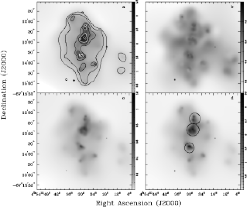
Figure 1: (a) Adaptively smoothed Chandra ACIS image, with surface brightness contours. Contours are logarithmically scaled over a factor of 20 from faintest to brightest emission. (b) Hardness ratio map H-S/H+S, using the soft and hard images below. (c) Soft-band ACIS image showing emission at 0.3-0.7 keV. (d) Hard-band ACIS image showing emission at 0.7-1.5 keV; regions used for the “bright ridge” spectrum are marked. The soft and hard X-ray images were adaptively smoothed on the same scale.

Figure 1a shows an image in the energy range 0.3–2.0 keV which contains almost all X-ray emission from the remnant. It has been adaptively smoothed with an algorithm that recognizes features with significance above 3$\sigma$. Contours of constant X-ray surface brightness are superposed on the image. Figure 1b shows a map of the hardness ratio, defined as H-S/H+S, where S is is emission from 0.3–0.7 keV (Figure 1c ) and H is emission from 0.7–1.5 keV (Figure 1d). The low dynamic range in the hardness ratio map demonstrates the spectral homogeneity across the SNR.

The remnant has dimension $2\farcm 3\times 3\farcm 6$ and is elongated in the NS direction. The brightest X-ray emission comes from a NS central ridge which includes three bright patches. 30% of the emission comes from these 3 regions. The brightest of these patches is almost central and 0$\farcm$4 in diameter. The surface brightness here is 5–10 times that of emission from the outer parts of the remnant. There is a hint of limb brightening in the north but otherwise little to indicate an X-ray emitting shell.

The optical morphology of SNR 0454$-$692 is highly filamentary (for first publication of MCELS images, see Smith et al., 1994). The filaments are distributed over a roughly elliptical region, with distortions toward the western side of the remnant. The H$\alpha$ emission from the SNR is superposed on a diffuse component possibly associated with the nearby H II region. The filamentary structure appears clearer in the [S II] $\lambda\lambda$6716, 6731 image, showing the cooled post-shock material. The [O III] emission outlines the rim of the SNR, more clearly delineating the expansion. The [S II] filaments appear slightly inward of the [O III]. This is expected for an expanding shell, as [O III] is produced in a temperature and density range that peaks closer to the shock front than the ranges for [S II] or H$\alpha$.

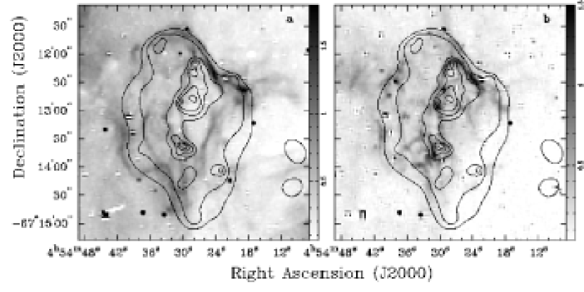
Figure 2: (a) Adaptively smoothed ACIS X-ray contours overlaid on a greyscale MCELS [O III] image. (b) ACIS contours overlaid on a greyscale MCELS [S II] image. Contours are scaled as in Fig. 1.

Figure 2a shows the X-ray contours overlaid on [O III] emission from the SNR, which nicely follows the X-ray boundary in the NW and SE. Figure 2b shows an overlay on [S II] emission. The [S II] emission follows the central ridge of brighter X-ray emission more strongly than the [O III] emission. To the SW, the X-rays appear to extend beyond the brightest optical emission. Figure 3a also displays the X-ray contours on [O III] emission, this time on a larger scale, to show the relationship of the SNR to the larger N9 region. Figure 3b shows X-ray contours overlaid on the 843 MHz radio emission for the same region. Although the radio resolution is limited, it can be seen that the basic structure of the radio emission corresponds well with that of the X-ray emission. The brightest part of the H II region to the northeast is also shown. The SNR is detectable at 4.8 GHz but is faint and hard to separate from the H II region.

The X-ray images also show a patch of very faint emission to the west, but no optical or radio counterpart to this emission is seen. Lacking any optical or radio evidence, we have chosen not to include this region as part of the remnant. However, it is certainly possible that this emission is in fact an extension of the SNR with connecting emission obscured by the dust lane seen in Figure 2a. Better radio data are needed to give a definite answer.

4 X-ray Spectra

Spectral fits were made to two regions: the three bright patches in the NS ridge and the faint diffuse structure filling the remainder of the remnant. (The three bright patches used for the central ridge are shown in Figure 1d.) A uniform distribution of material was assumed for each region. Although the advanced age of the SNR (see §6.1) suggests it may have reached ionization equilibrium (CIE), the X-ray spectra of other remnants have shown nonequilibrium ionization (NEI) effects to late SNR ages. We therefore fit the spectra with both NEI vpshock and CIE vmekal spectral models. For both models, abundances of all elements except H and He were set at 0.3 solar (typical for the LMC; Russel & Dopita, 1992) and abundances of O, Ne, and Fe allowed to vary. The ISM column density was fixed at $2\times 10^{21}$ atoms cm^-2 (Dunne 2004, personal communication, extracted from the H I survey of Kim et al., 2003). Results are listed in Table 1.

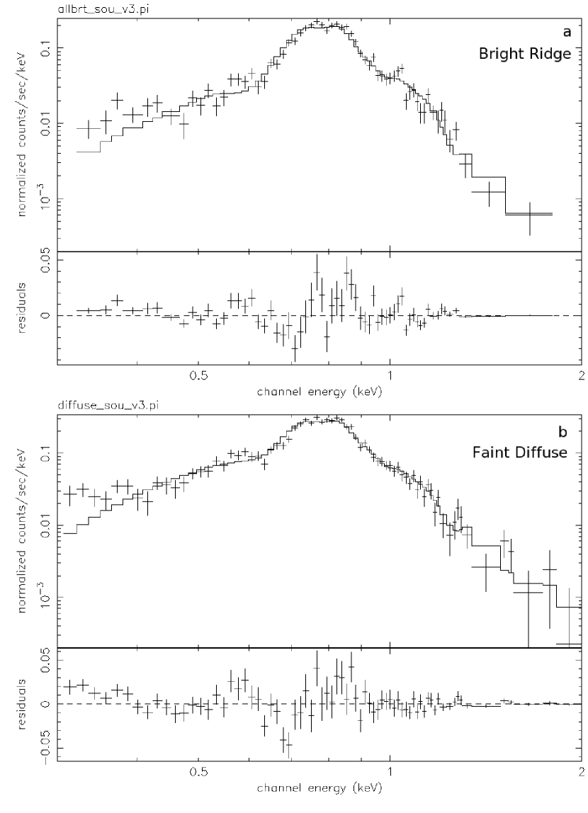
Figure 4: ACIS spectra from (a) the Bright Ridge of central emission, (b) the Faint Diffuse emission from the rest of the SNR.

Figure 4 shows the best fits to the spectra for the central ridge and the faint diffuse regions. The only significant difference in the spectra of the two regions is that the bright region has relatively more events in the range 0.65-0.9 keV than does the faint. This is where L-shell emission from Fe is concentrated and the difference is accounted for by adjusting the relative abundance of Fe. Abundances of O and Mg can be varied by up to 0.1 without making much difference to the fits. The temperature, however, is strongly dependent on the column density which was not allowed to vary.

The low ionization timescales ($\tau$) found for the NEI fits are somewhat surprising for a SNR of the dynamical age estimated in §6.1. If we freeze the timescale at a value consistent with CIE, and compare this fit to a fit in which the timescale is allowed to vary, an F-test between the two fit statistics shows the improvement to be significant. (The probability of no improvement is $1\times 10^{-11}$.)

To investigate variations between the volume emission measures of the three bright patches, the spectra were extracted separately for each of these regions, and then fit jointly with the best-fit model for the spectrum of the ridge as a whole. Only the normalizations, which are proportional to the volume emission measures ($\int n_{e}n_{H}dV$), were allowed to vary. The resulting volume emission measures are given in Table 2. Also given are estimated volumes occupied by the hot gas for each region. The bright patches are approximated by spherical volumes; for the northern region, we also did a volume estimate presuming that this region is part of the SNR shell. The faint diffuse emission is approximated by an ellipsoidal region with the line-of-sight dimension set equal to the minor axis, minus the volumes of the bright patches.

5 Compact Objects

The presence of interior neutron stars and their related PWN shows that gravitational collapse is the cause of some SN explosions. The association of a remnant and compact object also links both ages which can be difficult to evaluate separately. Many such associations should help us understand the evolution of these objects.

The LMC has been a fertile hunting ground. Three LMC remnants are known, through detection of pulsations, to have internal neutron stars: SNR 0540$-$69.3 and N 157B with Crab-like central objects and pulsars (Kaaret et al., 2001; Wang et al., 2001), and N 49 with an SGR considerably off center (Mazets et al., 1979; Evans et al., 1980; Rothschild, Kulkarni, & Lingenfelter, 1994). PWNe have been detected in two other SNRs, suggesting the presence of as yet undetected compact objects. SNR 0453$-$685 has a PWN at the center, but no unresolved source which might be the pulsar is detected (Gaensler et al., 2003). N 206 (0532$-$710) shows a faint X-ray shell surrounding bright thermal emission from the center. There is a weak compact X-ray source and PWN at one end of a linear radio feature, close to the rim of the remnant. Williams et al. (2005) propose this to be a fast moving neutron star leaving a radio wake.

The three neutron stars from which pulsations are seen are bright, with $L_{X}\approx 10^{36}$ erg s^-1. Fainter objects, however, would be harder to find. For example, there is a radio-quiet neutron star, or CCO for Central Compact Object, in the Galactic remnant Kes 79 (Seward et al., 2003) with $L_{X}=3\times 10^{33}$ erg s^-1 and a blackbody spectrum with kT $\sim 0.4$ keV, very similar to the central source in Cas A. (A 105 ms period has recently been detected in this CCO by Gotthelf et al., 2005, showing it to be an X-ray pulsar.) At a distance of 7 kpc, this CCO produced 700 counts in a 30 ks Chandra observation. Based on the greater distance but lesser column density of the LMC, we estimate that a 60 ks observation of this object in the LMC would yield 90 counts. So, in the LMC, a $10^{33}$ erg s^-1 CCO will yield 30 counts.

On the other hand, the Vela Pulsar, the faintest “young” pulsar with $L_{X}\approx 2\times 10^{32}$ erg s^-1, would be undetectable in the LMC. The absorption column density toward the LMC is an order of magnitude higher than that towards the Vela Pulsar, and thus the soft spectrum from such a pulsar would be absorbed. The surrounding PWN, however, has $L_{X}\approx 10^{33}$ erg s^-1 and a hard spectrum. It would have dimension of $0\farcs 5$ and would be seen, at the 30 count level, as an unresolved source. Thus, within the Magellanic Cloud remnants, we can easily detect central sources as faint as those found in the Milky Way. The upper limit for a point source imbedded in the bright center of this remnant is $\approx 5\times 10^{32}$ erg s${}^{-1}.$

The remnant under consideration here, 0454$-$672, shows no evidence for an energetic compact object. The morphology of the central bright region suggests a PWN but the X-ray spectrum from this region is similar to that of the rest of the remnant. In contrast, the PWN in 0453$-$685, which is younger, shows a distinctly nonthermal spectrum at both radio and X-ray wavelengths (Gaensler et al., 2003). There are seven nearby unresolved sources which are listed in Table 3. None are central to the remnant but, in an older remnant such as this, an initial kick could have moved the object to or beyond the boundary. The fourth source in the table, just inside the western boundary, is the best candidate for a CCO. Although neither intensity nor spectrum distinguishes it from a typical field source, a CCO similar to that found in Kes 79 is not ruled out. The sixth source in the table has a hard spectrum but is $3.3^{\prime}$ west of the remnant center, rather far away to have been associated with the SN.

6 Remnant Structure

6.1 Cool Ionized Shell

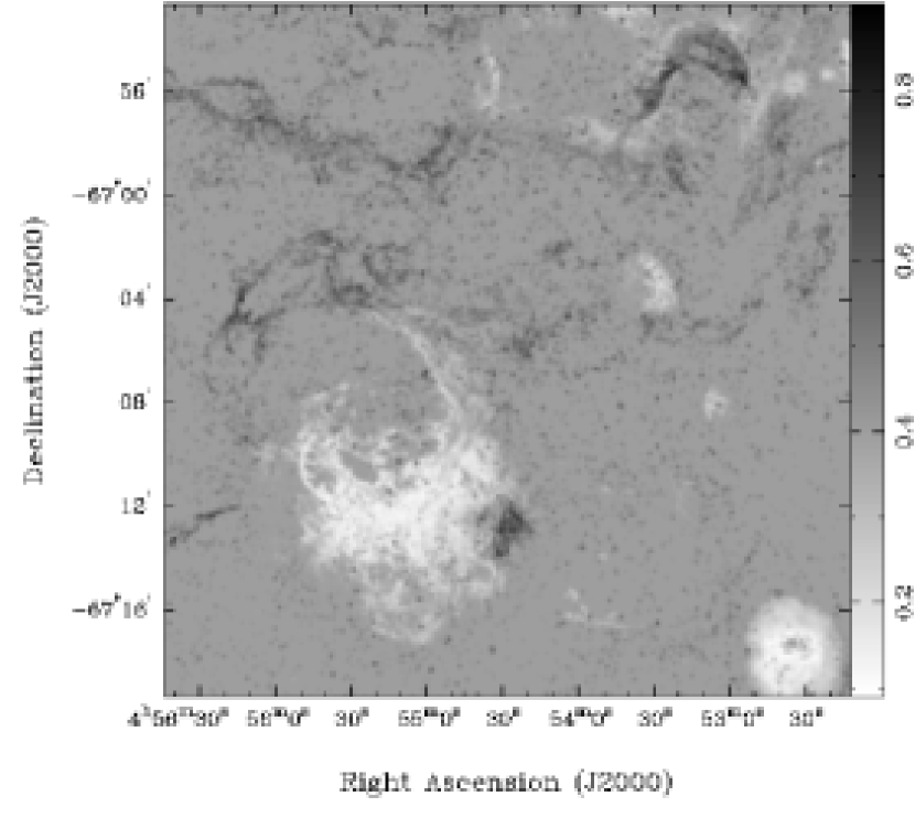
Figure 5: [S II]/H$\alpha$] map from flux-calibrated MCELS images. Input images were clipped at 2$\sigma$ of background. The final image has been smoothed by a Gaussian with $\sigma=2$. The sky background level has been set to 0.4, so shocked gas ([S II]/H$\alpha>0.4$) appears in black and photoionized gas ([S II]/H$\alpha<0.4$) appears in white. Some noise is present due to the residue from star subtractions. N9 is toward the bottom of the image, while the neighboring remnant in N4 is seen to the upper right.

We divided the flux-calibrated [S II] by H$\alpha$ to produce a [S II]/H$\alpha$ ratio map (Figure 5). This map shows an irregular inner region of filaments with [S II]/H$\alpha$ ratios of 0.6–0.8, with an outer “ring” of filaments with lower [S II]/H$\alpha$ ratios of 0.5–0.7, falling to 0.4 at the boundary between the SNR and the H II region. These ratios are very similar to those measured by Smith et al. (1994, Fig. 5,8d) for this SNR; as observed in that paper, these measured ratios are somewhat lower than the true ratios, due to contaminating emission from the background H II region.

To determine the density of the warm ionized shell of the N9 SNR, we have measured the average H$\alpha$ surface brightness of filaments to be (1–2) $\times 10^{-15}$ erg s^-1 cm^-2 arcsec^-2. The H$\alpha$ surface brightness can be converted to emission measure, $EM=\int n_{\rm e}^{2}dL$, where $n_{\rm e}$ is the electron density and $L$ is the length of the emitting material. Using the recombination coefficient for a 10⁴ K gas (Osterbrock, 1989) and assuming a filament’s length along the line of sight to be comparable to its length perpendicular to the line of sight, 44″ $\pm$ 8″, we find an rms electron density of $n_{\rm e}=8\pm 2$ cm^-3 in the SNR.

In the warm ionized gas, we assume He is singly ionized with a He to H number ratio of 0.1, and that the temperature of the gas is $\sim 10^{4}$ K. We can then use the electron density to calculate the thermal pressure in the shell: $P_{\rm th}=2.0n_{\rm e}kT=2.3\pm 0.4\times 10^{-11}$ dyne cm^-2. Similarly, we infer the mass of gas in the shell from our calculated electron density: $M_{\rm shl}=1.27n_{\rm e}m_{\rm H}V_{\rm shl}$, where $V_{\rm shl}$ is the shell volume. We assumed that the bulk of the warm ionized gas is distributed in a shell with thickness equal to the measured width of the filaments (1.0 $\pm$ 0.3 pc). Using this as the shell volume, we calculate the mass in such a shell to be $1300\pm 800M_{\sun}$. From high-dispersion echelle spectra of the H$\alpha$ and [N II] $\lambda\lambda$6548, 6583 lines, Chu (1997) estimated an average expansion velocity for the N9 SNR of $\sim 115\pm 5$ km s^-1. From this expansion velocity and our calculated shell mass, we determine a kinetic energy in the shell ($0.5M_{\rm shl}v_{\rm exp}^{2}$) of 1.7 $\pm 0.8\times 10^{50}$ erg.

We can also use this optical expansion velocity to estimate the age of the N9 SNR, using the simple expansion relationship $t=\eta R/v_{\rm exp}$, where $t$ is the SNR age and $R$ is its current radius. If we assume blast-wave expansion ($\eta=0.4$; Cox, 1972; Sedov, 1959) for this remnant, that velocity implies an age of 37,000 years; if we instead assume a pressure-driven snowplow model ($\eta=0.33$; Bandiera & Petruk, 2004), appropriate to the large size and interior X-ray emission, the calculated age drops to 31,000 years.

6.2 Hot Gas

The density of X-ray emitting material was calculated for three regions: the brightest central region - 17″ or 4.5 pc in radius; the faint diffuse interior; and the maximum in the north which might be a small part of the shell. These densities were calculated from the normalizations for the fitted X-ray spectral models, which are proportional to the volume emission measures. We assumed fully ionized H and He, with $n_{e}=1.2n_{H}$. Results are 0.66, 0.15, and 0.30-0.55 (dependent on geometry) electrons cm^-3 respectively. The X-ray emission from the interior implies a pressure of $\approx 1\times 10^{-10}$ dyne cm^-2, four times that derived for the filaments. The thermal energy of the hot interior gas is $\approx 3\times 10^{50}$ ergs. The observed sum of kinetic and thermal energy is therefore $\approx 5\times 10^{50}$ ergs which is a lower limit for $E_{0}$.

The ionization timescale for the diffuse interior, with the dynamical age calculated in §6.1, would imply a lower density of 0.06–0.07 cm^-3, rather than the higher value calculated from the X-ray normalization above. In part, this value may be an underestimate, as the optical velocity may not accurately represent the expansion of the remnant. If, for example, we took the X-ray emission as being generated behind the expanding shock, its temperature would imply a shock speed of 540 km s^-1 and (if approximately blast-wave expansion) an expansion speed of 400 km s^-1, which in turn would give a SNR age of about 22,000 yr. This age, combined with the ionization timescale, gives a density of about 0.1 cm^-3, closer to the emission-measure-derived value.

Conditions in the outer shell are not known. Obviously there is no X-ray limb brightening around most of the remnant. The shock has slowed to a point where material is shock-heated to temperatures of $T\leq 8\times 10^{5}$ K (0.07 keV), the approximate temperature below which the thermal X-rays are too soft to penetrate the ISM (Seward, 2000). In the absence of a clear PWN contribution, much of the interior emission can be attributed to “fossil” radiation - that is, emission from the low-density gas in the remnant interior (Seward, 1985; Rho & Petre, 1998) that was heated during earlier, more energetic stages of the SNR’s expansion. The prominent optical filaments show that the adiabatic phase is finishing and the remnant is now cooling. The age derived from the expansion of the filamentary shell is compatible with this. Estimates of the remnant parameters are summarized in Table 4.

The domination of a remnant by “fossil” radiation is one explanation often extended for the existence of “mixed morphology” SNRs, which have shell-like radio but centrally concentrated thermal X-ray emission, and lack a compact central source (e.g., Rho & Petre, 1998; Cox et al., 1999). N9 appears to fulfil at least two of these conditions. The X-ray data do not indicate a CCO (§5), and the radio spectrum for the SNR is not consistent with the presence of a PWN. Also, its X-ray morphology (§3) shows more prominent X-ray emission in the center than at the SNR limb, though the X-ray bright regions are distributed in a patchy, elongated fashion. On the other hand, it is difficult to determine a clear radio shell from the available data (Figure 3b), which makes this classification less certain. However, one must also take into account the low resolution of the radio images, and confusion with thermal emission from the H II region.

It is difficult to determine the kind of SN which produced this remnant. Because N9 is an H II region, the stellar population is expected to be young and any associated SN is expected to be Type II with consequent production of a neutron star; but there is no strong evidence for any compact object associated with SNR 0454$-$672. There is certainly no energetic pulsar within the remnant and the nearest unresolved X-ray source is 1$\farcm$2 from the center. If created at the center, this would require a velocity of $\approx 600$ km s^-1 to reach its present location, which is not an unreasonable velocity for a young neutron star. It is also not clear that a $3\times 10^{4}$ year old CCO would still be detectable or that the collapse did not create a black hole. Thus, we cannot rule out a Type II SN origin. The interior, however, shows signs of enhanced Fe abundance, consistent with a Type Ia SN origin. For example, the O/Fe number ratio in the SNR, based on our fitted abundances, is $\leq 1.3$, compared to a typical LMC ratio of 13.2 (based on Russel & Dopita, 1992). Models for the nucleosynthetic yields from Type Ia SNe suggest O/Fe ratios $<1$, while for Type II SNe the ratio is generally $\gtrsim 10$ (Iwamoto et al., 1999). Although the ratios in the SNR have large uncertainties and are affected by the presence of swept-up ISM, the relative contribution of iron appears to be significantly greater than one would expect from a Type II SN origin. This evidence is not as strong as in the case of DEM L71 (Hughes et al., 2003), but DEM L71 is a younger and brighter remnant.

Table 1: Best-fit spectral models to SNR regions

Parameter	Whole SNR		Bright Ridge		Faint Diffuse
component	vpshock	vmekal	vpshock	vmekal	vpshock	vmekal
kT (keV)	0.34${}^{+0.02}_{-0.01}$	0.206${}^{+0.012}_{-0.009}$	0.33${}^{+0.04}_{-0.02}$	0.21${}^{+0.02}_{-0.01}$	0.34${}^{+0.03}_{-0.01}$	0.20${}^{+0.01}_{-0.01}$
O/O☉	0.04${}^{+0.01}_{-0.01}$	0.004 ($<0.01$)	0.01 ($<0.04$)	0 ($<0.008$)	0.05${}^{+0.02}_{-0.02}$	0.012${}^{+0.014}_{-0.011}$
Ne/Ne☉	0.42${}^{+0.08}_{-0.07}$	0.29${}^{+0.08}_{-0.06}$	0.6${}^{+0.2}_{-0.2}$	0.5${}^{+0.2}_{-0.2}$	0.37${}^{+0.09}_{-0.08}$	0.26${}^{+0.09}_{-0.08}$
Fe/Fe☉	1.4${}^{+0.2}_{-0.1}$	0.8${}^{+0.1}_{-0.2}$	2.1${}^{+0.6}_{-0.2}$	1.2${}^{+0.5}_{-0.2}$	1.2${}^{+0.2}_{-0.2}$	0.7${}^{+0.2}_{-0.2}$
$\tau$ (cm-3 s)	8${}^{+3}_{-2}\times 10^{10}$	$\cdots$	1.1${}^{+0.7}_{-0.5}\times 10^{11}$	$\cdots$	7${}^{+5}_{-2}\times 10^{10}$	$\cdots$
norm (cm-5)	1.0${}^{+0.3}_{-0.2}\times 10^{-3}$	4.7${}^{+0.6}_{-0.5}\times 10^{-3}$	2.7${}^{+0.8}_{-0.9}\times 10^{-4}$	1.0${}^{+0.2}_{-0.2}\times 10^{-3}$	7${}^{+2}_{-2}\times 10^{-4}$	3.4${}^{+0.5}_{-0.2}\times 10^{-3}$
$\chi^{2}_{\rm red}$	1.48	1.88	1.72	2.26	1.21	1.44
dof	208	209	83	84	190	191

Note. — N_H is fixed to a value of $2\times 10^{21}$ cm^-2 from H I measurements for this pointing in the LMC (Kim et al., 2003) and the Galaxy (Dickey & Lockman, 1990). Spectra cover the range between 0.3-8.0 keV. Elements not listed are fixed to a LMC mean abundance of 30% solar (Russel & Dopita, 1992). Quoted errors are the statistical errors in each fit parameter at the 90% uncertainty level.

Table 2: X-ray Volume Emission Measures

Region	Vol. EM (cm-3)	Volume (cm3)
Northern bright	$2.0\times 10^{57}$	$7.9\times 10^{57}$
		$2.7\times 10^{58}$
Central bright	$4.1\times 10^{57}$	$1.1\times 10^{58}$
Southern bright	$1.6\times 10^{57}$	$5.7\times 10^{57}$
Faint diffuse	$2.1\times 10^{58}$	$1.1\times 10^{60}$

Table 3: Point Sources

RA(2000)	Dec (2000)	Counts (0.4-7 keV)	Counterpart	Comment
04 54 37.41	-67 14 48.4	41	none	$\cdots$
04 54 33.42	-67 14 50.9	18	yes	$\cdots$
04 54 29.20	-67 11 34.1	15	none?	$\cdots$
04 54 17.16	-67 13 13.4	22	none	inside remnant
04 54 15.43	-67 15 50.9	15	none	$\cdots$
04 54 00.14	-67 12 54.6	81	none?	hard spectrum
04 53 58.00	-67 13 35.8	61	yes, bright	soft spectrum

Table 4: Physical Properties of SNR 0454$-$672

Parameter	Value
X-ray luminosity (erg s-1)	$5.7\times 10^{35}$
Explosion energy (erg)	$\geq 4\times 10^{50}$
Age (yr)	$3\times 10^{4}$
Mass ($M_{\odot}$)	1300 in shell
	160 in interior hot gas
	7 in central 9 pc

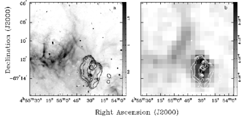
Figure 3: (a) Adaptively smoothed ACIS X-ray contours overlaid on a greyscale MCELS [O III] image. (b) ACIS contours overlaid on a greyscale image of 843 MHz radio emission. Contours are scaled as in Fig. 1. The larger shell to the northeast is from the neighboring N9 H II region.

References

- Bandiera & Petruk (2004) Bandiera, R. & Petruk, O. 2004, A&A, 419, 419
- Chu (1997) Chu, Y.-H. 1997, AJ, 113, 1815
- Chu & Kennicutt (1988) Chu, Y.-H. & Kennicutt, R.C. 1988, AJ, 96, 1874
- Cox (1972) Cox, D.P. 1972, ApJ, 178, 159
- Cox et al. (1999) Cox, D. P., Shelton, R. L., Maciejewski, W., Smith, R. K., Plewa, T., Pawl, A., & Różyczka, M. 1999, ApJ, 524, 179
- Dickel (1991) Dickel, J. 1991, in Woosley, S. ed., Supernovae, The tenth Santa Cruz Summer workshop in Astronomy and Astrophysics, (Berlin: Springer) 675
- Dickel et al. (2005) Dickel, J., McIntyre, V., Gruendl, R., & Milne, D. 2005, AJ, in press, February
- Dickey & Lockman (1990) Dickey, J. M., & Lockman, F. J. 1990, ARA&A, 28, 215
- Evans et al. (1980) Evans, W. D. et al. 1980, ApJ, 237, L7
- Filipovic et al. (1998) Filipovic, M. D. et al. 1998, A&AS, 127, 119
- Gaensler et al. (2003) Gaensler, B. M., Hendrick, S. P., Reynolds, S. P., & Borkowski, K. J. 2003, ApJ, 594, L111
- Gotthelf et al. (2005) Gotthelf, E. V., Halpern, J. P., & Seward, F. D. 2005, ApJ, 627, 390
- Haynes et al. (1991) Haynes, R., Klein, U.,Wayte, S., Wielebinski, R., Murray, J., Bajaja, E., Meinert, D., Buczilowski, U., Harnett, J., Hunt, A., Wark, R., & Sciacca, L. 1991, A&A, 252, 475
- Hendrick et al. (2003) Hendrick, S., Borkowski, K., & Reynolds, S. 2003, ApJ, 593, 370
- Hughes et al. (1995) Hughes, J.P. et al. 1995, ApJ, 444, L81
- Hughes et al. (1998) Hughes, J.P., Hayashi, I., & Koyama, K. 1998, ApJ, 505, 732
- Hughes et al. (2003) Hughes, J.P. Ghavamian, P., Rakowski, C.E., & Slane, P.O. 2003, ApJ, 582, L95
- Iwamoto et al. (1999) Iwamoto, K., Brachwitz, F., Nomoto, K., Kishimoto, N., Umeda, H., Hix, W. R., & Thielemann, F. 1999, ApJS, 125, 439
- Kaaret et al. (2001) Kaaret et al. 2001, ApJ, 546, 1159
- Kaspi & Helfand (2002) Kaspi, V. & Helfand, D. J. 2002, astro-ph/0201183
- Inoue et al. (1983) Inoue, H., Koyama, K., Tanaka, Y. 1983, in SNR and Their Emission, ed J. Danziger & P. Gorenstein, 535
- Kim et al. (2003) Kim, S., Staveley-Smith, L., Dopita, M. A., Sault, R. J., Freeman, K. C., Lee, Y., & Chu, Y.-H. 2003, ApJS, 148, 473
- Mazets et al. (1979) Mazets, E. P., Golentskii, S. V., Ilinskii, V. N., Aptekar, R. L., & Guryan, I. A. 1979, Nature, 282, 587
- Mathewson et al. (1984) Mathewson, D. S. et al. 1983, ApJS, 51, 345
- Osterbrock (1989) Osterbrock, C. 1989, Astrophysics of Gaseous Nebulae and Active Galactic Nuclei, (Mill Valley: University Science Books), Table 4.1
- Rho & Petre (1998) Rho, J. & Petre, R. 1998, ApJ, 503, L167
- Rothschild, Kulkarni, & Lingenfelter (1994) Rothschild, R. E, Kulkarni, S. R., & Lingenfelter, R. E. 1994, Nature, 368, 432
- Russel & Dopita (1992) Russel, S. C. & Dopita, M. A. 1992, ApJ, 384, 508
- Sedov (1959) Sedov, L. I. 1959, Similarity and Dimensional Methods in Mechanics (New York: Academic)
- Seward (1985) Seward, F. D. 1985, Comments Astrophys. XI, 1, 15
- Seward (2000) Seward, F. D. 2000, in Allen’s Astrophysical Quanties, ed. Arthur N. Cox (Springer, New York), pp. 193,195
- Seward et al. (2003) Seward, F. D., Slane, P., Smith, R., and Sun, M. 2003, ApJ, 584, 414
- Smith et al. (1994) Smith, R. C., Chu, Y.-H., Mac Low, M.-M., Oey, M. S. & Klein, U. 1994, AJ, 108, 1266
- Smith (2002) Smith, R.C., 2002, http://ctio.noao.edu/$∼$mcels/snrs/snrcat.html
- Smith et al. (1999) Smith, R. C. & The MCELS Team 1999, in IAU Symp. 190, New Views of the Magellanic Clouds, ed. Y.-H. Chu et al. (San Francisco: ASP), 28
- Wang et al. (2001) Wang, Q. D., Gotthelf, E. V., Chu, Y.-H., & Dickel, J. R. 2001, ApJ, 559 275
- Westerlund (1990) Westerlund, B. E. 1990, A&A Rev., 2, 29
- Williams et al. (2000) Williams, R. et al. 2000, ApJ, 536, L27
- Williams et al. (1999) Williams, R. et al. 1999, ApJS, 123, 467
- Williams et al. (2005) Williams, R. M., Chu, Y.-H., Dickel, J. R., Gruendl, R. A., Seward, F. D., Guerrero, M. A. & Hobbs, G. 2005, ApJ, 628, 704, astro-ph/0504609