Universe scenarios from loop quantum cosmology

Abstract.

Loop quantum cosmology is an application of recent developments for a non-perturbative and background independent quantization of gravity to a cosmological setting. Characteristic properties of the quantization such as discreteness of spatial geometry entail physical consequences for the structure of classical singularities as well as the evolution of the very early universe. While the singularity issue in general requires one to use difference equations for a wave function of the universe, phenomenological scenarios for the evolution are based on effective equations implementing the main quantum modifications. These equations show generic bounces as well as inflation in diverse models, which have been combined to more complicated scenarios.

1. Introduction

The universe is, on large scales, well described by general relativity which provides the basis for mathematical models of the possible behavior of a universe. From solutions of Einstein’s field equations one obtains the geometry of space-time once the matter content has been specified. On this classical level, however, the description will always remain incomplete as a consequence of singularity theorems: any space-time evolved backward in time from the conditions we perceive now will reach a boundary in a finite amount of proper time. At this boundary, the equations of the theory, and thus classical physics, break down, often accompanied by curvature divergence. For the development of complete universe scenarios the classical theory of general relativity thus has to be extended.

Such an extension is often expected to come from quantum gravity, where not only general relativistic but also quantum effects are taken into account. One approach, which is background independent and non-perturbative and can deal with those extreme conditions realized at classical singularities, is loop quantum gravity [1]. It is a canonical quantization and turns the classical metric and extrinsic curvature into operators on a Hilbert space. The classical geometrical structures are thus replaced by properties of operators which by itself leads to a different formulation. While classical geometry has to re-emerge as an approximation on large scales, on small scales quantum behavior has to be taken into account fully. (For general aspects of quantum theory in the context of cosmology see [2].) Then also the singularity problem appears in a different light as the basic object is not a space-time metric which cannot be extended beyond singularities in the classical evolution but a wave function. The wave function, also, is subject to equations which need to be analyzed in order to see if it always gives a complete solution telling us what happens at and beyond classical singularities.

Classical space-time is thus replaced by quantum space-time whose effects are most important on small scales such as those of a small universe close to a classical singularity. A fully quantized system is indeed necessary to describe states right at a classical singularity, but this is in general complicated at technical as well as conceptual levels. Close to classical singularities it is thus helpful to have effective systems which are of classical type, removing interpretational issues of quantum theories, but take into account some quantum effects. With those ingredients it is then possible to develop several complete scenarios for universes, and at the same time obtain potentially observable phenomenological effects.

2. Loop quantum cosmology

Just as Wheeler–DeWitt models, loop quantum gravity is a canonical quantization, i.e. it starts with a foliation of space-time into spatial slices $\Sigma_{t}$. Canonical variables are the spatial metric $q_{ab}$ and its momenta related to extrinsic curvature $K_{ab}$ of the slice [3]. The canonical Poisson algebra then is to be turned into a suitable operator algebra and represented on a Hilbert space. As always in field theories, however, operators for the field values in single points do not exist and the fields have to be smeared first by integrating them over extended regions. For field theories other than gravity, this is usually done on 3-dimensional regions using the background metric to define an integration measure. But for gravity, the metric itself is dynamical and thus to be smeared, and using an additional metric for smearing would introduce a background. A different procedure is required for gravity, i.e. we need to smear fields but do so in a background independent manner.

2.1. Holonomy-flux algebra

Indeed, the success of a quantization procedure often depends on the choice of basic variables. For gravity, it is most helpful to transform to new basic fields, given by Ashtekar variables [4, 5]. These variables are also canonical, but instead of the spatial metric one uses the densitized triad $E^{a}_{i}$, related to the spatial metric by $E^{a}_{i}E^{b}_{i}=\det qq^{ab}$, and the Ashtekar connection $A_{a}^{i}=\Gamma_{a}^{i}+\gamma K_{a}^{i}$ defined with the spin connection $\Gamma_{a}^{i}$ and extrinsic curvature components $K_{a}^{i}$. In addition, there is the Barbero–Immirzi parameter $\gamma>0$ [5, 6], which for simplicity will be set equal to one in what follows. (Its value can be computed from black hole entropy and is smaller than but of the order of one [7].) In those variables, the extrinsic curvature term in $A_{a}^{i}$ makes it canonically conjugate to the triad, and $\Gamma_{a}^{i}$ provides the transformation properties of a connection. For $E^{a}_{i}$, the important properties compared to the metric are that it also knows about the orientation of space since it can be left- or right-handed, and that it is dual to a 2-form $\epsilon_{abc}E^{c}_{i}$. The orientation will be essential later on in the discussion of singularities, while the transformation properties of a connection and dual 2-form, respectively, are important right now because they allow a natural smearing without introducing a background metric.

We can then integrate a connection along curves, where for good gauge properties we also take the path ordered exponential, i.e. use holonomies

$$h_{e}(A)={\cal P}\exp\int_{e}\tau_{i}A_{a}^{i}\dot{e}^{a}{\rm d}t$$ (1)

for curves $e\subset\Sigma$ and fluxes

$$F_{S}(E)=\int_{S}\tau^{i}E^{a}_{i}\epsilon_{abc}{\rm d}y^{a}{\rm d}y^{b}$$ (2)

for surfaces $S\subset\Sigma$. (SU(2)-generators $\tau_{j}=-\frac{1}{2}i\sigma_{j}$ with Pauli matrices $\sigma_{j}$ appear because this is the gauge group of triad-rotations not changing the metric.) There are then no 3-dimensional smearings, but a 1- and a 2-dimensional one, which, as it turns out, adds up to the right overall smearing for a well-defined quantization.

This is the basis of the background independent quantization provided by loop quantum gravity [8], and it has many crucial properties as direct consequences. First, the holonomy-flux algebra, defined by the Poisson relations, is, under weak mathematical conditions, represented uniquely on a Hilbert space together with a unitary action of diffeomorphisms of $\Sigma$ [9]. The latter property is required for the independence of gravity under the choice of spatial coordinates. This representation is cyclic, i.e. there is a basic state from which all others can be obtained by repeatedly acting with operators of the algebra. Other characteristic properties of the basic holonomy and loop operators are then very different from those in a Wheleer–DeWitt quantization: There is no operator for connection components or even their integrals, but only for holonomies unlike in a Wheeler–DeWitt quantization where extrinsic curvature components are basic operators. Moreover, flux operators have discrete spectra and so do geometrical operators such as area and volume [10]. With these properties, one can then use the basic representation to construct classes of well-defined Hamiltonian constraint [11]and matter Hamiltonian operators [12].

2.2. Isotropic quantum cosmology

These techniques also make a symmetry reduction possible which is much closer to the full theory than a Wheeler–DeWitt model would be [13]. When symmetries are imposed, natural sub-algebras of the full holonomy-flux algebra are defined which, using cyclicity of the representation, induce the basic representation of a model. Here, one simply acts only with those operators in the distinguished sub-algebra for a given symmetry, and thus obtains less states than one would get from the full holonomy-flux algebra. In this sense, the basic representation of models, which is so important for other physical properties, is directly obtained from the full quantum theory: quantization is done before performing the symmetry reduction, at least as far as the basic representation is concerned. More complicated operators such as the Hamiltonian constraint can then be constructed from the basic ones following the steps in the full theory by analogy.

The simplest case, isotropy, serves as a good example to illustrate the basic properties [14]. Classically, there is a single gravitational degree of freedom, the scale factor $a$ with its momentum $p_{a}=-3(4\pi G)^{-1}a\dot{a}$ ($G$ being the gravitational constant). These are components of the spatial metric and extrinsic curvature, which now are replaced by Ashtekar variables. In the isotropic case, there is again a single canonical pair $(c,p)$ with

$$|p|=a^{2}\qquad,\qquad{\rm sgn}(p)\mbox{: orientation}$$ (3)

and

$$c={\textstyle\frac{1}{2}}(k+\dot{a})\qquad,\qquad\mbox{$k=0$: flat, $k=1$: closed.}$$ (4)

These variables could be quantized directly in a Wheeler–DeWitt manner, i.e. $a$ as a multiplication operator and $\hat{p}_{a}=-i\hbar\partial/\partial a$ on square integrable functions (of only positive $a$, which means that $\hat{p}_{a}$ in this manner is not self-adjpoint), but an analog of the latter operator does not exist in the full theory. Through the induced holonomy-flux representation it is rather the exponentials $\exp(i\mu c/2)$ for any real $\mu$ (to be thought of as related to the parameter length of a curve) which are basic in addition to the densitized triad component $p$ proportional to a flux. The induced representation is then defined on a Hilbert space with orthonormal basis of states

$$\langle c|\mu\rangle=e^{i\mu c/2}\qquad,\qquad\mu\in{\mathbb{R}}$$ (5)

and basic operators

$$\hat{p}|\mu\rangle = {\textstyle\frac{1}{6}}\ell_{\rm P}^{2}\mu|\mu\rangle$$ (6)

$$\widehat{e^{i\mu^{\prime}c/2}}|\mu\rangle = |\mu+\mu^{\prime}\rangle\,.$$ (7)

Note that $\hat{p}$ is self-adjoint and $\widehat{e^{i\mu^{\prime}c/2}}$ is unitary since the full range of real numbers for $\mu$ is allowed taking into account the orientation freedom in a triad. In this representation, basic operators of the model have the same properties as those in the full theory [15]: $\hat{p}$ has normalizable eigenstates and thus a discrete spectrum (nonetheless, the set of eigenvalues is the full real line, which is not in conflict with the discreteness of the spectrum because the Hilbert space is non-separable) and one can see that there is no operator for $c$ but only for exponentials $e^{i\mu c/2}$ not being continuous in $\mu$.

Compared to a Wheeler–DeWitt quantization, however, the properties are very different. In that case, the scale factor, related to $p$, would have a continuous spectrum and extrinsic curvature $p_{a}$, related to $c$, would be represented directly as an operator. The properties realized in loop quantum cosmology as in the full theory are a consequence of strong restrictions coming from background independence and its transfer to symmetric models.

On this basic representation we can construct more complicated operators, most importantly the Hamiltonian constraint. Since the properties of basic operators are as in the full theory, the construction can be done in an analogous manner, only adapting to the symmetric context where needed. Properties of composite operators are then also close to those in the full theory, although for them the relation, as of now, is not as tight and there is no derivation of symmetric composite operators from the full ones.

For the Hamiltonian constraint, we start from the classical Friedmann equation

$$H=-6\left[2c(c-k)+k^{2}\right]\sqrt{|p|}+8\pi GH_{\rm matter}(p,\phi,p_{\phi})=0$$

with matter Hamiltonian $H_{\rm matter}$, e.g.

$$H_{\phi}=\frac{1}{2}a^{-3}p_{\phi}^{2}+a^{3}V(\phi)$$ (8)

for a scalar $\phi$ with momentum $p_{\phi}$ and potential $V(\phi)$, written down in isotropic Ashtekar variables. This is, using the volume operator $\hat{V}=|\hat{p}|^{3/2}$ with eigenvalues

$$V_{\mu}=(\ell_{\rm P}^{2}|\mu|/6)^{3/2}$$ (9)

and replacing factors of $c$ by exponentials (7), quantized to an operator equation $\hat{H}|\psi\rangle=0$ for states $|\psi\rangle=\sum_{\mu}\psi_{\mu}(\phi)|\mu\rangle$ given by a difference equation [14, 16, 15] such as

$$(V_{\mu+5}-V_{\mu+3})e^{ik}\psi_{\mu+4}(\phi)-(2+k^{2})(V_{\mu+1}-V_{\mu-1})\psi_{\mu}(\phi)$$ (10)

$$+(V_{\mu-3}-V_{\mu-5})e^{-ik}\psi_{\mu-4}(\phi)=-{\textstyle\frac{4}{3}}\pi G\ell_{\rm P}^{2}\hat{H}_{\rm matter}(\mu)\psi_{\mu}(\phi)$$

for $\psi_{\mu}(\phi)$. Unlike Wheeler–DeWitt equations which are differential, there is thus a difference equation as a result of discrete quantum geometry. Nevertheless, for large $\mu\gg 1$ the difference operators can be expanded in a Taylor series provided that the wave function is sufficiently differentiable [17, 15]. This property can be included in semiclassicality conditions [18, 19], but in more complicated models the existence of sufficiently differentiable solutions may not be guaranteed [20].

2.3. Classical singularities

With the propagation equation for the wave function on minisuperspace we can now address the issue of singularities in quantum cosmology. Compared to the classical situation, the setup has changed since we do not have evolution equations for the metric in coordinate time, but an equation for the wave function on minisuperspace. In semiclassical regimes, the metric can be reconstructed from the wave function, for instance making use of observables (as completed for a free, massless scalar in [21]). But it is not guaranteed that a classical geometric picture is suitable everywhere for the behavior of a universe. From the point of view of quantum gravity, the propagation equation for the wave function is more fundamental, and so also the singularity issue is to be addressed at this level. The question then arises whether or not initial values in one classical regime of large volume are sufficient to determine the quantum solution on all of (mini)superspace including regions which can be interpreted as being beyond a classical singularity. If this is the case, quantum space-time would not be incomplete and thus non-singular.

For isotropic quantum cosmology, this question can be answered immediately. Minisuperspace is, first of all, enlarged compared to the usual metric space in that we have two regions differing by their orientation ${\rm sgn}(p)$ and separated by degenerate geometries. Classically, they are thus separated by singularites. In quantum theory, the configuration space for wave functions $\psi_{\mu}(\phi)$ also knowns about orientation via ${\rm sgn}(\mu)$, and a classical singularity would occur at $\mu=0$. Unlike the classical evolution, the quantum equation for the wave function uniquely yields the wave function on one side if we pose initial values on the other side. In this way, aspects of quantum gravity give us, first, a new region of minisuperspace and, second, a unique extension between the two regions. In this manner, quantum gravitational models are singularity-free [22]. So far, explicit constructions include anisotropic (Bianchi class A) models [23, 24] and as inhomogeneous cases spherical symmetry and polarized cylindrical gravitational waves [25, 26].

The criterion of extendability used here is the most direct and most general one for the singularity issue, both at the classical as well as quantum level. In quantum cosmology, other criteria have been used such as the finiteness of the wave function at a classical singularity. Also this is realized automatically in loop quantum cosmology because, thanks to discreteness, there is always only a finite number of computational steps between initial values and a classical singularity. Infinities in the wave function could then only arise from diverging matter Hamiltonians, which does not occur in loop quantizations as we will explain more explicitly in what follows. In this context, we will also discuss curvature divergence which sometimes serves as a singularity criterion.

At a more intuitive level, we obtain the picture of a universe which starts in a collapsing branch and evolves through a phase where continuous geometry fails but discrete quantum geometry remains meaningful. At the transition, the orientation of space changes implying that the universe turns its inside out. What exactly happens during the transition depends on the concrete matter model. If one has a parity violating matter Hamiltonian such as that of the standard model, there are changes between the two branches even in the equations of motion. Otherwise, the two sides generically are still different from each other depending on the initial conditions for the wave function. Even if one starts close to a classical geometry on one side, it may then happen that after evolving through a violent quantum regime a new classical geometry will not be recovered. This does, however, not happen in matter models with a free, massless scalar which can be treated completely [21]. In this case, solutions which are semiclassical for large volume bounce at small volume and become semiclassical afterwards. For those solutions, there is no difference in behavior when the orientation is changed.

As already noted, the difference equation can be well approximated by the usual Wheeler–DeWitt equation on large scales. On small scales, the equations differ considerably, but in some cases one can still compare the effects of initial conditions. For the Wheeler–DeWitt equation, initial conditions have originally been imposed at $a=0$ with the intention of removing the classical singularity by requiring the wave function to vanish there [27, 28]. However, this turns out to be ill-posed as an initial value problem, i.e. in most models only the trivial solution of a vanishing wave function exists. In loop quantum cosmology, on the other hand, dynamical initial conditions have been derived from the difference equation [18, 29] which in many cases are comparable to DeWitt’s condition $\psi(0)=0$ but making it well-posed in the discrete setting [30]. For a closed model, one can see [31] that the dynamical initial conditions are closer to the no-boundary proposal [32] than to the tunneling proposal [33]. But also in the discrete setting, the situation is more complicated in less symmetric models such as anisotropic [20] or inhomogeneous ones [26] where analogous mechanisms are more difficult to realize. The possibility of conditions following from the constraint equation also depends on the ordering of the Hamiltonian constraint operator which may change coefficients in the difference equation. The ordering for (10) as also used in [18] is not symmetric, and using a symmetric one removes additional conditions for wave functions in isotropic models. Symmetric orderings are often required for semiclassical issues or for computing the physical inner product, and moreover for a non-singular evolution in inhomogeneous models [26]. In such a situation, isotropic models loose their dynamical initial conditions, but some conditions remain in anisotropic models [34] as well as the inhomogeneous case. Here, however, the analysis of implications for the solution space is still very incomplete. A general mechanism to provide initial conditions for the wave function of a universe is thus still outstanding.

2.4. Matter Hamiltonian

For a complete cosmological model, we also need to know its matter content and quantize its Hamiltonian for quantum cosmology. This, now, does not only include the matter fields but also geometrical factors in a matter Hamiltonian which need to be turned into operarors. For instance for a scalar, the Hamiltonian $H_{\phi}=\frac{1}{2}{a^{-3}}p_{\phi}^{2}+a^{3}V(\phi)$ has to become an operator in the field values $\phi$ but also in the scale factor $a$. We thus need a quantization of the inverse of $a$, or $p$, in order to quantize the kinetic term.

At this point, properties of the basic representation become important: As we have seen, a loop quantization leads to an operator $\hat{p}$ which has a discrete spectrum containing zero, and such an operator does not have a densely defined inverse. This seems to be a severe obstacle, but it turns out that well-defined quantizations do exist [35], just as well-defined matter Hamiltonians exist in the full theory [12]. In quantizations, the most obvious procedure is not always the successful one, and also here one has to start from alternative expressions for $a^{-3}$ which are identical classically but lead to different quantizations.

One can rewrite $a^{-3}$ as, e.g.,

$$a^{-3}=\left(\frac{3}{8\pi G{lj}({j}+1)(2{j}+1)}\sum_{I=1}^{3}{\rm tr}_{j}(\tau_{I}h_{I}\{h_{I}^{-1},|p|^{l}\})\right)^{3/(2-2{l})}$$ (11)

with parameters $0<l<1$ and $j\in\frac{1}{2}{\mathbb{N}}$, using only positive powers of $p$ and “holonomies” $h_{I}=e^{c\tau_{I}}$ of the connection component $c$. Inserting the basic operators and turning the Poisson bracket into a commutator, this can directly be quantized to a well-defined operator with eigenvalues [36, 37]

$$\widehat{d(a)}_{\mu}^{(j,l)}=\left(\frac{9}{\ell_{\rm P}^{2}lj(j+1)(2j+1)}\sum_{k=-j}^{j}k|p_{\mu+2k}|^{l}\right)^{3/(2-2l)}\,.$$ (12)

As one can see, the eigenvalues do depend on the parameters $j$ and $l$, unlike the classical expression. Rewriting in the above manner thus introduces ambiguities as it is expected for the quantization of any non-basic operator. Important properties are, however, robust. For instance, for any choice of the parameters we obtain the classical behavior of $a^{-3}$ at large values $\mu\gg j\ell_{\rm P}^{2}$, a peak around $\mu_{*}=j\ell_{\rm P}$ and decreasing behavior on small scales reaching exactly zero for $\mu=0$.

For larger $j$, the sum in the eigenvalues contains many terms, and it can be approximated by viewing it as a Riemann sum of an integral. In this way, we obtain the effective density

$$d(a)^{(j,l)}_{\rm eff}:=\widehat{d(a)}_{\mu(a^{2})}^{(j,l)}=a^{-3}p_{{l}}(3a^{2}/{j}\ell_{\rm P}^{2})^{3/(2-2{l})}$$ (13)

with $\mu(p)=6p/\ell_{\rm P}^{2}$ and

$$\textstyle p_{l}(q) \textstyle= \textstyle\frac{3}{2l}q^{1-l}\left(\frac{1}{l+2}\left((q+1)^{l+2}-|q-1|^{l+2}\right)\right.$$ (14)

$$\textstyle\qquad-\left.\frac{1}{l+1}q\left((q+1)^{l+1}-{\rm sgn}(q-1)|q-1|^{l+1}\right)\right)\,.$$

The approximation becomes better for larger $j$ as the number of terms in the Riemann sum increases, which can also be seen in Fig. 2.4.

[htb] Discrete sets of eigenvalues of $\widehat{d(a)}_{\mu}^{(j,l)}$ for two values of $j$ and $l=3/4$ compared to the classical behavior $a^{-3}$, the approximations by $d(a)_{\rm eff}^{(j,l)}$ and small-$a$ power-law approximations.

Analogous constructions of $d(a)$ exist, e.g. $d(a_{1},a_{2},a_{3})$ in anisotropic models with diagonal metric components $g_{II}=a_{I}^{2}$. In contrast to an isotropic context, these functions are not required to be bounded for all configurations, i.e. all $a_{I}$ (see, e.g., [38]). The isotropic situation is very special in the way the approach to the classical singularity at $a=0$ happens for which there is only one possible trajectory in minisuperspace (which can only be followed with different rates in coordinate time $t$). In less symmetric models, there is much more freedom in the approach such as $a_{I}(t)$ in anisotropic models, and not all possible configurations are realized along the generic approach. Also in the full theory, degenerate configurations exist on which inverse volume operators have unbounded expectation values [39]. At this point, dynamical information has to be used to find out if curvature remains bounded along effective trajectories of universe models.

[htb] Curvature potential on the minisuperspace of a diagonal Bianchi IX model with one metric component held fixed. Curvature is unbounded on minisuperspace, in particular at large anisotropies. Close to classical singularities (center and diagonal lines at $x=0$ or $y=0$), however, it remains bounded.

This can be done in homogeneous models such as the Bianchi IX model [24] where curvature is unbounded on all of minisuperspace (Fig. 2.4) but bounded along the effective and even quantum evolution as given by the difference equation. On smaller scales, also deviations from the classical approach happen which imply non-chaotic behavior as the curvature walls start to break down from quantum effects [40, 41]. From this, one can draw conclusions for the generic inhomogeneous approach and structure formation using the BKL picture [42], but for definitive conclusions inhomogeneous models have to be studied in more detail and in particular perturbative schemes for structure formation.

2.5. Effective equations

Difference equations, in particular partial ones in the presence of matter fields or ansiotropies and inhomogeneities, are difficult to deal with, and also interpretational issues of the wave function arise at this level. While the full quantum setting is needed to discuss singularities and the discrete evolution in their vicinity, on larger scales it is more direct to use effective equations of classical type. Those equations are differential equations in coordinate time, but they are amended by modifications to capture quantum effects. This is analogous to effective action techniques, and indeed there is a general scheme for effective classical approximations of quantum systems [43, 44] which can be applied to quantum cosmology in a canonical formulation and reproduces the usual effective action results [45] obtained by expanding around free field theories or the harmonic oscillator [44].

This scheme is based on a geometrical formulation of quantum mechanics [46] where the Hilbert space is interpreted as an infinite dimensional vector space with additional structure. The infinite dimensionality, even for a mechanical system, is the crucial difference between quantum and classical physics. There are thus additional quantum degrees of freedom which in some regimes have to be taken into account (often appearing as higher derivative terms in effective actions). From the inner product of the Hilbert space one obtains a symplectic structure as well as a metric on the vector space such that it becomes Kähler. In addition, the quantum Hamiltonian defines a flow on the Kähler manifold. With the symplectic structure and the flow one has a canonical system equivalent to the quantum system and in general involving all infinitely many degrees of freedom. In some cases, however, it is possible to approximate the flow by a dynamical system on a finite dimensional subspace of the full space, giving rise to an effective classical system. This may involve only the classical degrees of freedom, but with correction terms in the evolution, or also additional ones related to, e.g., the spread of wave functions. The metric on the Kähler space is needed only for the measurement process in quantum mechanics and issues such as the collapse or overlap of wave functions. Since there is no external observer in quantum cosmology and only one wave function, the metric may be dropped which means that one could, as mentioned in [2], weaken the Hilbert space structure required usually. Indeed, the geometrical formulation of quantum mechanics provides a unified scheme for generalizations of quantum mechanics [46].

In loop quantum cosmology, several related methods have been applied in order to derive effective terms for equations of motion, although a complete derivation is still unfinished. The geometrical scheme is developed for quantum cosmology in [43] with an asymptotic series of correction terms for isotropic models. Leading orders of such terms have also been derived in [47] and with WKB techniques in [48]. Some of these terms have been used in applications [49, 50, 51, 47], but many effects already show up at the level where additional degrees of freedom are considered only to the lowest order. The order of differential equations is then the same as classically, but terms in the Hamiltonian do change. In particular, the quantum Hamiltonian requires, in the presence of matter or other curvature terms, a quantization of $a^{-3}$ which is modified at the quantum level. Effectively, $a^{-3}$ in the matter Hamiltonian is replaced by $d(a)$ from (13) [52]:

$$H_{\phi}(a)=\frac{1}{2}d(a)p_{\phi}^{2}+a^{3}V(\phi)$$ (15)

which behaves differently from the classical expression for $a<\sqrt{j/3}\ell_{\rm P}$.

From the matter Hamiltonian we obtain Hamiltonian equations of motion for the matter field, which now change on small scales [16]. For a scalar, we have the effective Klein–Gordon equation

$$\ddot{\phi}=\dot{\phi}\,\dot{a}\frac{\mathrm{d}\log{d(a)}}{\mathrm{d}a}-a^{3}{d(a)}V^{\prime}(\phi)$$ (16)

where the usual friction term $-3\dot{\phi}\dot{a}/a$ changes its form. Back-reaction from matter on geometry is encoded in the Friedmann equation which also changes. Substituting the effective matter Hamiltonian, we obtain the effective Friedmann equation

$$a(\dot{a}^{2}+k^{2})={\textstyle\frac{8\pi}{3}}G\left({\textstyle\frac{1}{2}}{d(a)}\,p_{\phi}^{2}+a^{3}V(\phi)\right)$$ (17)

and from the equations of motion generated by the constraint the effective Raychaudhuri equation

$$\frac{\ddot{a}}{a}=-\frac{8\pi G}{3}\left(a^{-3}{d(a)}p_{\phi}^{2}\left(1-{\textstyle\frac{1}{4}}a\frac{{\mathrm{d}}\log(a^{3}{d(a)})}{{\mathrm{d}}a}\right)-V(\phi)\right)\,.$$ (18)

In the latter, the modification leads to an entirely new term.

3. Phenomenology

These equations, all resulting from a single modification in the matter Hamiltonian implied by effects of the basic quantum representation, are the starting point for phenomenology of loop cosmology based on effective equations. Additional corrections, related to quantum fluctuations and additional quantum degrees of freedom, have not yet been studied systematically but are expected to be important only on very small scales. Modifications in the matter Hamiltonian, on the other hand, are non-perturbative and can be shifted into regimes of larger scales just by choosing a large value for $j$. This allows one to study its implications in isolation from other correction terms, even though one does not expect $j$ to be very large. Additional corrections [48, 47] and similar parameters [51] also arise for the gravitational part of the constraint and become relevant when the matter density is large (of Planck size).

The main modification can then easily be interpreted intuitively by viewing the Friedmann equation as the energy equation of a classical mechanics system with a potential determined by the matter Hamiltonian. Classically, the matter Hamiltonian is usually decreasing as a function of $a$ as a consequence of the kinetic term. This is a consequence of the fact that classical gravity is always attractive. When $a^{-3}$ is replaced by $d(a)$ as in Fig. 2.4, however, the slope of the potential is flipped on small scales and it becomes increasing. Thus, the direction of the force changes and (quantum) gravity on small scales receives a repulsive contribution. With this picture, one can easily imagine that characteristic effects can arise such as the prevention of collapse into a singularity by a bounce or the acceleration of expanding evolution to an inflationary era.

3.1. Bounces

For a bounce to be realized, we need to find a time where $\dot{a}=0$ and $\ddot{a}>0$. The first condition can be checked with the effective Friedmann equation (17) where, for $\dot{a}=0$ to be possible, the positive kinetic term must be compensated by either a positive curvature term $k=1$ [53, 54] or a negative scalar potential $V(\phi)<0$ [55]. The second condition at solutions for $\dot{a}=0$ is then controlled by the effective Raychaudhuri equation (18) which for classical solutions gives only negative $\ddot{a}$, i.e. recollapse points.

When a turning point falls in the modified regime, on the other hand, the additional term in the effective Raychaudhuri equation as well as modified matter behavior through the effective Klein–Gordon equation (16) can change the picture and imply bounces. This is not realized in all cases, but happens generically and without the need for special potentials in contrast to the classical situation. Numerical solutions for two examples are given in Fig. 1. These effective bounces can be seen as a consequence of a repulsive gravitational force, or equivalently of negative pressure

$$P=-\frac{\partial H}{\partial V}=-\frac{1}{3a^{2}}\frac{\partial H}{\partial a}<0$$ (19)

which changes sign on scales where the matter Hamiltonian is increasing.

Figure 1. Numerical solutions (solid lines) for bounces in models with positive spatial curvature (left) and a negative potential (right), respectively, compared to the classically singular solutions (dashed).

The modification in the matter Hamiltonian alone does not give rise to bounces in all cases, such as a flat model with positive potential. A universe then still collapses to small sizes closer and closer to the deep quantum regime. Eventually, its dynamics has to be described by the basic difference equation which is non-singular, but at small sizes also additional corrections become important in effective equations. Those corrections are indeed directly related to the underlying discreteness or quantum fluctuations of geometry, and appear on very small scales. This, then, provides bounces more generically [50, 56, 49, 21].

3.2. Inflation

Negative pressure is also required for inflation where $\ddot{a}>0$ can now follow without special conditions for the potential or the initial values of an inflaton field. In fact, inflation in the general sense of accelerated expansion now happens generically and even without any potential at all [52] as illustrated in Fig. 3.2. It is enough that the kinetic term in the effective Friedmann equation becomes increasing as a function of $a$ which is always realized on small scales.

[htb] Numerical solution with inflationary behavior (right) in the regime of modified effective densities (left). Dashed lines indicate the range of sizable modifications.

The precise manner depends on the ambiguity parameter $l$ for which we obtain $d(a)\sim{a^{3/(1-l)}}$ on small scales which is always increasing due to $0<l<1$. This form determines, for a vanishing potential, the type of inflation which is super-inflationary (with equation of state parameter $w=-1/(1-l)<-1$). For more realistic models with a potential, however, the behavior is driven very close to exponential inflation thanks to the $a$-dependence of the potential term [57]. From the behavior of matter in such an inflating background one can then derive potentially observable effects.

We first look at the kinetic term driven inflation which happens for any matter field and thus can eliminate the need for an inflaton. During accelerated expansion in this regime, structure can be generated with less fine tuning than in inflaton models. As preliminary calculations indicate [58], the resulting spectrum is nearly scale invariant [57], and quantum effects can also be used to give arguments, based on [59, 60], for a small amplitude in agreement with observations. Details of the spectrum such as the running of the spectral index do depend on ambiguity parameters such that they may be restricted by forthcoming detailed observations. In contrast to single field inflaton models, the spectral index would be a little larger than one as a consequence of super-inflation, i.e. the spectrum is slightly blue, which can be a characteristic signature.

If this phase alone would have to be responsible for the generation of all structure, an extremely large value for the parameter $j$ would be required. Moreover, the spectrum would then be blue on all scales which is ruled out by observations. As we will see now, however, the first inflationary phase will always be followed by slow-roll phases because matter (or inflaton) fields are driven away from their potential minima while the modified Klein–Gordon equation is active. Subsequent phases can thus serve to make the universe large enough and provide a sufficient amount of $e$-foldings, while visible structure can have been generated in the first, quantum phase. Attractive features of this class of scenarios are that potentials for matter fields driving late-time slow-roll phases do not need to be special and that visible structure would have been generated by the quantum phase, thus giving potentially observable quantum signatures.

3.3. Scalar dynamics

In the effective Klein–Gordon equation (16) the classical friction term of an expanding universe, used for slow-roll behavior, changes sign and turns into an antifriction term on small scales [52]. Matter fields in this regime are then excited and can move up their potential walls even if they start close to minima at small momenta. After antifriction subsides, they will continue to roll up the walls but be slowed down by the then active friction. Eventually, they turn around and roll down the potential slowly. In this manner, additional phases of inflation are generated. The whole history is shown in Fig. 2 with a rapid initial phase containing the push of $\phi$ up its potential and the loop inflationary phase together with the later slow-roll stage. A solution for the scale factor showing both inflationary phases in the same plot is given in Fig. 2.

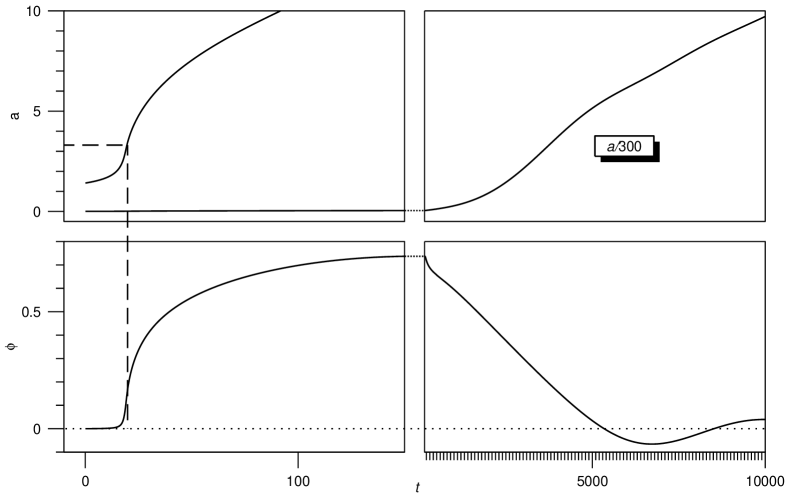
Figure 2. Initial push of a scalar field $\phi$ up its potential with subsequent slow-roll to and oscillations around the potential minimum at $\phi=0$.

If $\phi$ is an inflaton such as that of chaotic inflation with a quadratic potential, initial conditions are provided for a long phase of slow-roll inflation. But the slow-roll conditions are not satisfied in all stages, in particular not around the turning point of the inflaton. Here, $\dot{\phi}$ vanishes or is very small such that the slow-roll condition $\ddot{\phi}\ll H\dot{\phi}$ cannot be satisfied. If the second phase is responsible for structure formation, structure on large scales, generated in early stages of the slow-roll phase, will differ from usual scenarios. This can in particular contribute to a suppression of power on large scales [61]. If the last inflationary phase takes too long these effects are not visible, but one can estimate the duration from the inflaton initial values one typically gets through the antifriction mechanism. As it turns out, one often obtains observable effects, i.e. there is a sufficient amount of inflation but not too much for washing away quantum gravity effects [62]. This aspect is even enhanced if one looks at the evolution at the level of difference equations [63].

[htb] Numerical solution showing the first inflationary phase of loop cosmology and the beginning of the ensuing slow-roll phase after the scalar is pushed up its potential.

3.4. Combinations of different phases

So far we have considered individual bounces or inflationary phases. Depending on details of the matter system such as potentials, many combinations are possible and often of interest for model building. If one combines several bounces in models with a classical recollapse, oscillatory models result [64]. The behavior can then gradually change from cycle to cycle and eventually, after small changes have added up, result in a qualitative change in the universe behavior.

This is realized, for instance, in a new version of the emergent universe which was originally devised as a non-singular inflationary model with positive spatial curvature [65]. The singularity is avoided by starting the model close to a static Einstein space in the infinite past which, with a suitable potential, develops into an inflationary phase. The initial state is, however, very special because the static Einstein space is unstable. This changes if effective equations of loop cosmology are used: there are new static solutions on small scales which, in contrast to the classical ones, are stable [66]. Starting close to those solutions will lead to a series of cycles of a small universe which can gradually change due to the motion of matter fields in their potential.

In this manner, one obtains a whole history for a universe evolving through different phases of contraction and expansion in a cyclic but not necessarily periodic manner. However, the cycles are usually short and do not automatically give rise to a large universe. On the other hand, matter fields move in their potential during the evolution, and close to bounce points antifriction effects can help to bring matter fields far up their potentials or over potential barriers. If a suitable part of the potential is encountered during this process, the conditions can be right for the start of a slow-roll regime of sufficient duration for a large universe to emerge [67]. In fact, this can be obtained in the emergent universe scenario from a simple initial state evolving, after many cycles, to an inflationary phase for the structure formation we need for our universe [66, 68]. A numerical solution for this scenario is illustrated in Fig. 3.4. The characteristic feature is that it is based in an essential manner on closed spatial slices of positive curvature which, if the inflationary phase is not too long, may be detectable in the near future [66].

[htb] Stroboscopic density plot of solutions in the classical phase space (arbitrary units) with initial cyclic behavior and an eventual inflationary phase. To illustrate the time behavior, Gaussians have been added peaked at discrete coordinate time intervals.

When different matter sources are present, such as different fields or a fluid in addition to a scalar field, other possibilities arise. There can still be fixed points which allow cyclic behavior around them, but the position can now depend on the field values. In particular, cyclic motion of the fixed points themselves is possible which implies that the evolution is double-cyclic with small cycles around a fixed point superposed to the cyclic motion of the fixed point [69]. There are several new possibilities which are being investigated in dynamical system approaches. In this context it is in particular of interest when a graceful entrance into an inflationary phase can arise in the presence of different matter sources, i.e. how generically initial conditions become right to start a sufficiently long slow-roll phase.

Cyclic behavior is also studied often in the context of brane collisions. While loop quantum gravity and cosmology are difficult to formulate in this higher-dimensional setting, one can simply take potentials motivated from brane scenarios [71] and study implications with loop modifications. The interpretation of the scalar is then as a radion field, i.e. the distance between two branes. A common characteristic property is the possibility of negative potentials which, as we have seen earlier, allow bounces in loop cosmology.

Loop cosmology then provides a non-singular bounce for such a brane model, and one can check how easy it is to realize properties assumed in other models where a mechanism for singularity removal was not known. In some of those scenarios, for instance, it was assumed that the scale factor bounces and simultaneously the scalar field turns around [72]. Only then does one really have a model where the branes first approach each other and then bounce off. This turns out to be impossible in loop cosmology based on (17) where bounces are realized with a negative potential but, as illustrated in Fig. 3, the scalar cannot change direction [55]. The only possibility for $\phi$ to turn around is if it encounters a region of positive potential, but then one automatically obtains an inflationary phase and the scenario is not different from those described before. Similar results can be obtained when bouncing solutions realized with higher curvature corrections are used [73].

Figure 3. Bouncing numerical solution for the scale factor (left) in a brane potential with a monotonic decrease of the scalar (right). During bounces, the scalar is only slowed down due to antifriction in the effective Klein–Gordon equation, but it cannot turn around. A turnaround can be realized only if the scalar encounters positive values of its potential, which generically leads to inflation (dashed).

4. Conclusions

Through its background independent and non-perturbative quantization scheme, loop quantum gravity and cosmology are well-equipped for extreme physical situations as they are realized close to classical singularities. With symmetric models, those situations can now be dealt with in many cases including cosmology and black holes. Many examples exist for non-singular models by the same general mechanism, and also conceptual problems can be solved. In addition, many phenomenological applications arise from a few basic effects.

These effects have, in all cases, been known first from mathematical considerations and then transferred to and evaluated explicitly in models. The discussed effects then resulted automatically, rather than being looked for with particular applications in mind. Moreover, a few effects going back to properties of the basic representation dictated by background independence suffice to cover a plethora of physical applications in different areas.

This fact is encouraging for the viability of the whole framework, but it is still important to understand the relation between models and the full theory as completely as possible. Some properties can directly be related, and others have to be derived after analogous constructions. There are no known contradictions, but at the dynamical level also no proof of, e.g., singularity removal without assuming symmetries. It is, however, clear already that the presence of local physical degrees of freedom is by itself no obstacle to non-singular quantum evolution.

Also models, in particular inhomogeneous ones, have to be developed in more detail. At the fundamental level one then has to deal with many coupled partial difference equations, for which even the formulation of a well-posed initial or boundary value problem can be difficult. For solutions one will have to refer to new numerical techniques which are being developed in investigations of numerical quantum gravity. Effective equations would also help considerably in understanding inhomogeneous situations, but their derivation is much more complicated than in homogeneous models and so far not completed.

At the same time, properties of the full theory are being understood better. There is thus an approach from two sides, by weakening symmetries in models to get closer to the full setting and by starting to understand full configurations which can be argued to be close to states considered in a symmetric model. A third direction will, in the future, be provided by observations and their relation to phenomenological results. In this way, confidence in physical effects derived with loop methods will be strengthened and can eventually be compared with observations.

References

- [1] A. Ashtekar and J. Lewandowski, Class. Quantum Grav. 21, R53 (2004); C. Rovelli, Quantum Gravity (Cambridge University Press, Cambridge, UK, 2004); T. Thiemann, gr-qc/0110034.
- [2] C. Kiefer, these Proceedings or gr-qc/0508120.
- [3] R. Arnowitt, S. Deser, and C. W. Misner, in Gravitation: An Introduction to Current Research, edited by L. Witten (Wiley, New York, 1962).
- [4] A. Ashtekar, Phys. Rev. D 36, 1587 (1987).
- [5] J. F. Barbero G., Phys. Rev. D 51, 5507 (1995).
- [6] G. Immirzi, Class. Quantum Grav. 14, L177 (1997).
- [7] A. Ashtekar, J. C. Baez, A. Corichi, and K. Krasnov, Phys. Rev. Lett. 80, 904 (1998); A. Ashtekar, J. C. Baez, and K. Krasnov, Adv. Theor. Math. Phys. 4, 1 (2000); M. Domagala and J. Lewandowski, Class. Quantum Grav. 21, 5233 (2004); K. A. Meissner, Class. Quantum Grav. 21, 5245 (2004).
- [8] C. Rovelli and L. Smolin, Nucl. Phys. B 331, 80 (1990).
- [9] H. Sahlmann, gr-qc/0207111; gr-qc/0207112; H. Sahlmann and T. Thiemann, gr-qc/0302090; gr-qc/0303074; A. Okołów and J. Lewandowski, Class. Quantum Grav. 20, 3543 (2003); C. Fleischhack, math-ph/0407006; J. Lewandowski, A. Okołów, H. Sahlmann, and T. Thiemann, gr-qc/0504147.
- [10] C. Rovelli and L. Smolin, Nucl. Phys. B 442, 593 (1995), erratum: Nucl. Phys. B 456, 753 (1995); A. Ashtekar and J. Lewandowski, Class. Quantum Grav. 14, A55 (1997); A. Ashtekar and J. Lewandowski, Adv. Theor. Math. Phys. 1, 388 (1997).
- [11] T. Thiemann, Class. Quantum Grav. 15, 839 (1998).
- [12] T. Thiemann, Class. Quantum Grav. 15, 1281 (1998).
- [13] M. Bojowald and H. A. Kastrup, Class. Quantum Grav. 17, 3009 (2000).
- [14] M. Bojowald, Class. Quantum Grav. 19, 2717 (2002).
- [15] A. Ashtekar, M. Bojowald, and J. Lewandowski, Adv. Theor. Math. Phys. 7, 233 (2003).
- [16] M. Bojowald and K. Vandersloot, Phys. Rev. D 67, 124023 (2003).
- [17] M. Bojowald, Class. Quantum Grav. 18, L109 (2001).
- [18] M. Bojowald, Phys. Rev. Lett. 87, 121301 (2001).
- [19] M. Bojowald and G. Date, Class. Quantum Grav. 21, 121 (2004).
- [20] D. Cartin, G. Khanna, and M. Bojowald, Class. Quantum Grav. 21, 4495 (2004); D. Cartin and G. Khanna, Phys. Rev. Lett. 94, 111302 (2005); G. Date, Phys. Rev. D 72, 067301 (2005).
- [21] A. Ashtekar, T. Pawlowski, and P. Singh, in preparation.
- [22] M. Bojowald, Phys. Rev. Lett. 86, 5227 (2001).
- [23] M. Bojowald, Class. Quantum Grav. 20, 2595 (2003).
- [24] M. Bojowald, G. Date, and K. Vandersloot, Class. Quantum Grav. 21, 1253 (2004).
- [25] M. Bojowald, Class. Quantum Grav. 21, 3733 (2004).
- [26] M. Bojowald, Phys. Rev. Lett. 95, 061301 (2005).
- [27] B. S. DeWitt, Phys. Rev. 160, 1113 (1967).
- [28] H. D. Conradi and H. D. Zeh, Phys. Lett. A 154, 321 (1991).
- [29] M. Bojowald, Gen. Rel. Grav. 35, 1877 (2003).
- [30] M. Bojowald and F. Hinterleitner, Phys. Rev. D 66, 104003 (2002).
- [31] M. Bojowald and K. Vandersloot, in Xth Marcel Grossmann meeting (World Scientific, 2003).
- [32] J. B. Hartle and S. W. Hawking, Phys. Rev. D 28, 2960 (1983).
- [33] A. Vilenkin, Phys. Rev. D 30, 509 (1984).
- [34] A. Ashtekar and M. Bojowald, gr-qc/0509075.
- [35] M. Bojowald, Phys. Rev. D 64, 084018 (2001).
- [36] M. Bojowald, Class. Quantum Grav. 19, 5113 (2002).
- [37] M. Bojowald, in Proceedings of the International Conference on Gravitation and Cosmology (ICGC 2004), Cochin, India, Pramana 63, 765 (2004).
- [38] M. Bojowald, gr-qc/0508118.
- [39] J. Brunnemann and T. Thiemann, gr-qc/0505033.
- [40] M. Bojowald and G. Date, Phys. Rev. Lett. 92, 071302 (2004).
- [41] M. Bojowald, G. Date, and G. M. Hossain, Class. Quantum Grav. 21, 3541 (2004).
- [42] V. A. Belinskii, I. M. Khalatnikov, and E. M. Lifschitz, Adv. Phys. 13, 639 (1982).
- [43] A. Ashtekar, M. Bojowald, and J. Willis, in preparation; J. Willis, Ph.D. thesis, The Pennsylvania State University, 2004.
- [44] E. S. Fradkin and A. A. Tseytlin, Nucl. Phys. B 261, 1 (1985).
- [45] M. Bojowald and A. Skirzewski, math-ph/0511043.
- [46] A. Ashtekar and T. A. Schilling, in On Einstein’s Path: Essays in Honor of Engelbert Schücking, edited by A. Harvey (Springer, New York, 1999), pp. 23–65.
- [47] P. Singh and K. Vandersloot, Phys. Rev. D 72, 084004 (2005).
- [48] G. Date and G. M. Hossain, Class. Quantum Grav. 21, 4941 (2004); K. Banerjee and G. Date, Class. Quant. Grav. 22, 2017 (2005).
- [49] M. Bojowald, P. Singh, and A. Skirzewski, Phys. Rev. D 70, 124022 (2004).
- [50] G. Date and G. M. Hossain, Phys. Rev. Lett. 94, 011302 (2005).
- [51] K. Vandersloot, Phys. Rev. D 71, 103506 (2005).
- [52] M. Bojowald, Phys. Rev. Lett. 89, 261301 (2002).
- [53] P. Singh and A. Toporensky, Phys. Rev. D 69, 104008 (2004).
- [54] G. V. Vereshchagin, JCAP 07, 013 (2004).
- [55] M. Bojowald, R. Maartens, and P. Singh, Phys. Rev. D 70, 083517 (2004).
- [56] G. Date, Phys. Rev. D 71, 127502 (2005).
- [57] G. Date and G. M. Hossain, Phys. Rev. Lett. 94, 011301 (2005).
- [58] G. M. Hossain, Class. Quantum Grav. 22, 2511 (2005).
- [59] T. Padmanabhan, Phys. Rev. Lett. 60, 2229 (1988).
- [60] T. Padmanabhan, T. R. Seshadri, and T. P. Singh, Phys. Rev. D 39, 2100 (1989).
- [61] S. Tsujikawa, P. Singh, and R. Maartens, Class. Quantum Grav. 21, 5767 (2004).
- [62] M. Bojowald et al., Phys. Rev. D 70, 043530 (2004).
- [63] A. Ashtekar, P. Singh, and K. Vandersloot, in preparation.
- [64] J. E. Lidsey, D. J. Mulryne, N. J. Nunes, and R. Tavakol, Phys. Rev. D 70, 063521 (2004).
- [65] G. F. R. Ellis and R. Maartens, Class. Quant. Grav. 21, 223 (2004); G. F. R. Ellis, J. Murugan, and C. G. Tsagas, Class. Quant. Grav. 21, 233 (2004).
- [66] D. J. Mulryne, R. Tavakol, J. E. Lidsey, and G. F. R. Ellis, Phys. Rev. D 71, 123512 (2005).
- [67] D. J. Mulryne, N. J. Nunes, R. Tavakol, and J. Lidsey, Int. J. Mod. Phys. A 20, 2347 (2005).
- [68] M. Bojowald, Nature 436, 920 (2005).
- [69] N. J. Nunes, Phys. Rev. D 72, 103510 (2005).
- [70] E. J. Copeland, J. E. Lidsey, and S. Mizuno, gr-qc/0510022.
- [71] R. Maartens, Living Rev. Rel. 7, 7 (2004), http://www.livingreviews.org/lrr-2004-7.
- [72] J. Khoury, B. A. Ovrut, P. J. Steinhardt, and N. Turok, Phys. Rev. D 64, 123522 (2001); P. J. Steinhardt and N. Turok, Phys. Rev. D 65, 126003 (2002).
- [73] S. Tsujikawa, Class. Quant. Grav. 20, 1991 (2003).