Neutrino spectrum from the pair-annihilation process in the hot stellar plasma

Abstract

An new method of calculating the energy spectrum of neutrinos and antineutrinos produced in the electron-positron annihilation processes in hot stellar plasma is presented. Detection of these neutrinos, produced copiously in the presupernova which is evolutionary advanced neutrino-cooled star, may serve in future as a trigger of pre-collapse early warning system. Also, observation of neutrinos will probe final stages of thermonuclear burning in the presupernova.

The spectra obtained with the new method are compared to Monte Carlo simulations. To achieve high accuracy in the energy range of interest, determined by neutrino detector thresholds, differential cross-section for production of the antineutrino, previously unknown in an explicit form, is calculated as a function of energy in the plasma rest frame. Neutrino spectrum is obtained as a 3-dimensional integral, computed with the use of the Cuhre algorithm of at least 5% accuracy. Formulae for the mean neutrino energy and its dispersion are given as a combination of Fermi-Dirac integrals. Also, useful analytical approximations of the whole spectrum are shown.

I Introduction & Motivation

We present here a new method which allows us to calculate the spectrum of neutrinos produced by thermal pair-annihilation processes in the hot plasma in the core of massive pre-supernova star. The paper is organized as follows: In sect.II the electron-positron pair annihilation processes into neutrinos in the Standard Model are briefly summarized. Monte Carlo simulations are discussed in section III.1. Simple estimates of the average energy of neutrinos based on the Dicus cross-section Dicus (1972) are presented in Subsection III.2.

The complete spectrum is obtained using the differential cross-section (Eq. (31)) derived in Subsection III.3, where the spectrum is given in the form of three dimensional integral, that is easy to evaluate numerically with the Cuhre or Monte Carlo algorithms. Additionally, we express the moments of the spectrum as a combination of Fermi-Dirac integrals (Subsection III.4), that are used to obtain convenient analytical approximation of the spectrum in Subsect. III.5.

Our long-term goal is to explore the entire neutrino spectrum produced by massive stars at late nuclear burning stages. Unlike the Sun, these stars after carbon ignition emit both neutrinos from weak nuclear reactions and thermal neutrinos. Moreover, photon luminosity is negligible compared to neutrino luminosity and therefore these objects are referred to as neutrino-cooled stars Arnett (1996). Neutrinos emitted as neutrino-antineutrino pairs dominate up to the silicon burning Woosley et al. (2002). The electron antineutrinos are much easier to detect than neutrinos Odrzywolek et al. (2004a, b); Beacom and Vagins (2004); Oberauer (private communication). We consider them first.

Production of pair-annihilation neutrinos is the dominant thermal process with relatively high average neutrino energy of $\langle\mathcal{E}_{\nu}\rangle\sim$1.5 MeV. However, the information on neutrino emission is not complete without full knowledge of all neutrino processes. This is important because other neutrino processes can also produce low energy neutrinos which are difficult to detect. These neutrinos somehow ”steal” detectable energy from the stellar core reducing chances for e.g. supernova prediction.

The results presented here are general in nature, and are valid for pair-annihilation neutrinos from $e^{+}e^{-}$ plasma in the full range of temperature and chemical potential.

II Pair annihilation in the Standard Model

According to the Standard Model of electroweak interactions, the electron-positron pair may annihilate not only into photons but also into neutrino-antineutrino pair:

$$e^{+}+e^{-}\longrightarrow\nu_{x}+\bar{\nu}_{x}.$$ (1)

In the first order calculations, sufficient in the considered energy range of several MeV ($E\ll$ M${}_{W^{\pm},Z^{0}}$ where M${}_{W^{\pm},Z^{0}}$ is the intermediate boson mass of $\sim$100 GeV), two Feynmann diagrams (Fig. 1) contribute to the annihilation amplitude.

   

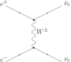
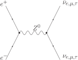
Figure 1: Feynmann diagrams leading to the first-order amplitude for $e^{+}e^{-}$ annihilation into neutrinos. Electron neutrinos are produced via both diagrams, while $\mu$ and $\tau$ neutrinos only by “$Z^{0}$ decay”.

The contribution from the left diagram in Fig. 1, i.e. $W^{\pm}$ boson exchange (charged current) is given by Dicus (1972):

$$-\frac{iG_{F}}{\sqrt{2}}\bar{u}_{\nu}\gamma^{\alpha}(1-\gamma_{5})u_{e}\;\bar{v}_{e}\gamma_{\alpha}(1-\gamma_{5})v_{\nu}.$$ (2)

This part of the process produces only electron neutrinos. Using the Fierz transformation:

$$\bar{a}[\gamma^{\mu}(1-\gamma_{5})]b\;\bar{c}[\gamma_{\mu}(1-\gamma_{5})]d=-\bar{a}[\gamma^{\mu}(1-\gamma_{5})]d\;\bar{c}[\gamma_{\mu}(1-\gamma_{5})]b$$ (3)

we may write (2) as :

$$-\frac{iG_{F}}{\sqrt{2}}\bar{u}_{\nu}\gamma^{\alpha}(1-\gamma_{5})v_{\nu}\;\bar{v}_{e}\gamma_{\alpha}(1-\gamma_{5})u_{e}.$$ (4)

The $Z^{0}$ boson exchange (neutral current) gives:

$$-\frac{iG_{F}}{\sqrt{2}}\bar{u}_{\nu}\gamma^{\alpha}(1-\gamma_{5})v_{\nu}\;\bar{v}_{e}\gamma_{\alpha}(g_{V}-g_{A}\;\gamma_{5})u_{e}\quad$$ (5)

where:

$$g_{V}=-\frac{1}{2}+2\sin^{2}{\theta_{W}},\qquad g_{A}=-\frac{1}{2}$$

By adding (4) to (5) we obtain the total annihilation amplitude:

$$\mathcal{M}=-\frac{iG_{F}}{\sqrt{2}}\bar{u}_{\nu}\gamma^{\alpha}(1-\gamma_{5})v_{\nu}\;\bar{v}_{e}\gamma_{\alpha}(C_{V}^{f}-C_{A}^{f}\;\gamma_{5})u_{e}.$$ (6)

Here $G_{F}=1.16637(1)\times 10^{-5}\,\mbox{GeV}^{-2}$ is the Fermi constant of weak interactions Eidelman et al. (2004). The parameters $C_{V}^{f}$ and $C_{A}^{f}$ ($f=e,\mu,\tau$ – neutrino flavor) in the Standard Model of the electroweak interactions are:
for electron neutrinos:

$$C_{V}^{e}=\frac{1}{2}+2\sin^{2}{\theta_{W}},\qquad C_{A}^{e}=\frac{1}{2}$$ (7)

for $\mu$ and $\tau$ neutrinos:

$$C_{V}^{\mu,\tau}=-\frac{1}{2}+2\sin^{2}{\theta_{W}},\qquad C_{A}^{\mu,\tau}=-\frac{1}{2},$$ (8)

where $\theta_{W}$, the Weinberg angle, is $\sin^{2}{\theta_{W}}=0.22280\pm 0.00035$ Eidelman et al. (2004).

As the pair-annihilation into electron neutrinos proceeds via both charged and neutral currents we have:

$$C_{V}^{e}=C_{V}^{\mu,\tau}+1,\qquad C_{A}^{e}=C_{A}^{\mu,\tau}+1$$ (9)

Annihilation into $\mu$ and $\tau$ neutrinos proceeds via the neutral current only.

In general, the entire spin-averaged information on $e^{+}e^{-}$ annihilation process (1) is included in the spin-averaged ($\sigma_{i}$ - spin states) squared annihilation matrix $M^{2}$:

$$M^{2}\equiv\overline{|\mathcal{M}|^{2}}=\frac{1}{2}\frac{1}{2}\sum_{\sigma_{e^{+}},\sigma_{e^{-}}}\sum_{\sigma_{\nu},\sigma_{\bar{\nu}}}|\mathcal{M}|^{2}.$$ (10)

The amplitude $M^{2}$ can be calculated using e.g. the Casimir trick:

$$M^{2}=8{G_{F}}^{2}\Big{\{}\left(C_{A}^{f}-C_{V}^{f}\right)^{2}P_{1}\cdot Q_{1}\,P_{2}\cdot Q_{2}\\ +\left(C_{A}^{f}+C_{V}^{f}\right)^{2}P_{2}\cdot Q_{1}\,P_{1}\cdot Q_{2}\\ +{m_{e}}^{2}\left({C_{V}^{f}}^{2}-{C_{A}^{f}}^{2}\right)\,Q_{1}\cdot Q_{2}\Big{\}}$$ (11)

where $P_{1}=(E_{1},\mathbf{p}_{1})$, $P_{2}=(E_{2},\mathbf{p}_{2})$, $Q_{1}=(\mathcal{E}_{1},\mathbf{q}_{1})$ $Q_{2}=(\mathcal{E}_{2},\mathbf{q}_{2})$ is, respectively, the four-momentum of the electron, positron, neutrino and antineutrino.

According to the definition of the cross-section $d\sigma$, the number of collisions $dN$ occurring in volume $dV$ in time $dt$ is Landau and Lifshitz (1975):

$$\frac{dN}{dVdt}=d\sigma v\;dn_{1}\;dn_{2},$$ (12)

where $dn_{1,2}$ are particle densities. In the case of two incoming particles, the differential cross-section can be computed from the Fermi Golden Rule formula and is given by the expression Griffiths (1987):

$$d\sigma v=\frac{1}{2E_{1}}\frac{1}{2E_{2}}\frac{1}{(2\pi)^{2}}\;\delta^{4}(P_{1}+P_{2}-Q_{1}-Q_{2})\;\frac{d^{3}\mathbf{q}_{1}}{2\mathcal{E}_{1}}\frac{d^{3}\mathbf{q}_{2}}{2\mathcal{E}_{2}}\;M^{2}.$$ (13)

Hence, if $M^{2}$ is known, the total neutrino emissivity from ${e^{+}}{e^{-}}$ plasma can be calculated by performing appropriate integrations Yakovlev et al. (2001):

$$\frac{4}{(2\pi)^{8}}\int\frac{d^{3}\mathbf{p}_{1}}{2E_{1}}\frac{d^{3}\mathbf{p}_{2}}{2E_{2}}\frac{d^{3}\mathbf{q}_{1}}{2\mathcal{E}_{1}}\frac{d^{3}\mathbf{q}_{2}}{2\mathcal{E}_{2}}\Lambda\;f_{1}f_{2}\;\delta^{4}(P_{1}+\ldots)\;M^{2}.$$ (14)

Substituting into the integrand of (14) the appropriate expression for the factor $\Lambda$ we obtain formulae for the number emissivity ($\Lambda=2$), the total emissivity (the energy carried by neutrinos and antineutrinos) ($\Lambda=E_{1}+E_{2}=\mathcal{E}_{1}+\mathcal{E}_{2}$), the antineutrino emissivity ($\Lambda=\mathcal{E}_{2}$) etc. Functions $f_{1},f_{2}$ are the Fermi-Dirac distributions for electrons and positrons, respectively:

$$f_{1}=\frac{1}{e^{(E_{1}-\mu)/kT}+1},\qquad f_{2}=\frac{1}{e^{(E_{2}+\mu)/kT}+1},$$ (15)

where $\mu$ is the electron chemical potential (including the rest mass) and neutrinos and antineutrinos are assumed to escape freely from the plasma.

The total neutrino emissivity, as required e.g. for stellar evolution codes, including the emission of all three flavors ($e,\mu,\tau$) is the sum of three terms of the form of the integral (14) with appropriate coefficients (7, 8) in (11).

The formal expression (14) must be transformed into analytical or convenient numerical form before actual application for e.g. stellar evolution codes or signal estimations in neutrino detectors. The integral (14) above is simplified significantly if Lenard’s formula Lenard (1953a, b):

$$\int\frac{d^{3}\mathbf{q}_{1}}{2\,\mathcal{E}_{1}}\frac{d^{3}\mathbf{q}_{2}}{2\,\mathcal{E}_{1}}\;Q_{1}^{\alpha}Q_{2}^{\beta}\;\delta^{4}(P_{1}+P_{2}-Q_{1}-Q_{2})=\frac{\pi}{24}\left[g^{\alpha\beta}(P_{1}+P_{2})^{2}+2\;(P_{1}^{\alpha}+P_{2}^{\alpha})(P_{1}^{\beta}+P_{2}^{\beta})\right]\Theta\left[(P_{1}+P_{2})^{2}\right]$$ (16)

is applied to integrate over outcoming neutrino momenta giving the well-known cross section of Dicus (1972) for annihilation of the $e^{-}e^{+}$ pair with four-momenta $P_{1}$ and $P_{2}$:

$${\sigma v}_{D}=\frac{{G_{F}}^{2}}{12\pi}\frac{{m_{e}}^{4}}{E_{1}E_{2}}\Biggl{[}\left({C_{V}^{f}}^{2}+{C_{A}^{f}}^{2}\right)\left(1+3\;\frac{P_{1}\cdot P_{2}}{{m_{e}}^{2}}+2\;\frac{(P_{1}\cdot P_{2})^{2}}{{m_{e}}^{4}}\right)+\left({C_{V}^{f}}^{2}-{C_{A}^{f}}^{2}\right)\left(1+2\;\frac{P_{1}\cdot P_{2}}{{m_{e}}^{2}}\right)\Biggr{]}$$ (17)

The formula (14) can be now transformed using (17) into:

$$\frac{4}{(2\pi)^{6}}\int d^{3}\mathbf{p}_{1}d^{3}\mathbf{p}_{2}\;\Lambda\;{\sigma v}_{D}\;f_{1}f_{2}.$$ (18)

In contrast to a more general Eq. (14), in (18) $\Lambda$ must be a function of $e^{-},e^{+}$ momenta $\mathbf{p}_{1},\mathbf{p}_{2}$ only, and we are unable to compute the antineutrino spectrum separately. The expression (18) above is actually a three-dimensional integral – due to the rotational symmetry only lengths and angle between $\mathbf{p}_{1}$ and $\mathbf{p}_{2}$ are independent variables of integration. Therefore, (18) may be integrated, leading to a combination of Fermi-Dirac integrals (cf. Sect. III.2) which are easily computed numerically.

We can obtain the total neutrino luminosity in this way. Unfortunately, if one attempts to consider the detection of these neutrinos very important information about the neutrino energy is missing. Detection efficiency depends strongly on the neutrino energy – higher energy neutrinos are much easier to detect – so the spectrum parameters and the shape actually decide whether these neutrinos will be observed or not. Therefore we must go back to the general formula (14) and try to attack it in an another way. We consider various possible approaches in the next subsections.

III Neutrino spectrum

III.1 Monte Carlo simulations

The Monte Carlo simulation is a method often used to calculate annihilation spectra. We applied it in our previous work Odrzywolek et al. (2004a), with some minor errors in the algorithm. To improve the calculations we develop semi-analytical methods, to make cross-check of the obtained results. Poor accuracy for higher energies of previously obtained results did not allow us to compute reliably the spectrum for energies E$>$4 MeV. Using better random number generator, namely Mersenne Twister routine Matsumoto and Nishimura (1998), and longer simulation runs, we were able to extend the spectrum to 6-7 MeV at least, but accuracy was still unacceptable, cf. Fig. 2.

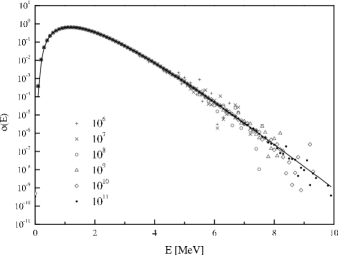
Figure 2: Spectrum resulting from the Monte Carlo simulation for $10^{6},10^{7},10^{8},10^{9},10^{10}$ and $10^{11}$ loop size (symbols) versus spectrum from (37) computed with aid of Cuhre algorithm (solid line, relative accuracy 0.05). We can notice decreasing errors of the Monte Carlo simulation near the maximum and increasing number of events in the high energy tail. Obviously, the Monte Carlo simulation is unable to reach accuracy of Cuhre methods for $E\gg$5 MeV. This figure clearly justifies efforts to compute the spectrum using the appropriate cross-section (31), instead of using Monte Carlo simulation based on the knowledge of the annihilation matrix (11). We would like to point out that three-dimensional integral (37) may also be computed using advanced Monte Carlo adaptive algorithms, giving similar spectra much faster, but they may fail in some cases, cf. Fig. 3. Spectrum computed for typical situation in stellar center during Si burning with $T=0.319$ MeV and $\mu=0.85+m_{e}$ MeV,

As we can see in Fig. 2 the Monte Carlo simulation reproduces the spectrum well. Unfortunately, this method is very slowly convergent: time required to compute the grid of neutrino spectra for e.g. the purpose of integrating them over the entire volume of the hot stellar core is very long. Moreover, the accuracy of this method is limited by resolution of the random number generator, and errors in the interesting range above $\sim$5 MeV (Super-Kamiokande threshold) are large. Therefore development of the analytical formulae is welcome. Nevertheless, Monte Carlo simulations based only on the amplitude $M^{2}$ (11) may be used even in the case where analytical formula for the cross-section is not available.

III.2 Emissivity and average neutrino energy

Some quantities related to the neutrino emission process, such as reaction rates, the total emissivity and the average neutrino energy, can be easily obtained directly from the Dicus cross-section (17) as electron energy moments. These quantities are average values for $\nu-\bar{\nu}$ pair. However, in Sect. III.3 we show how to modify average values by small additive terms to obtain the relevant quantities for neutrinos and antineutrinos separately. This becomes possible only using a more general cross-section (31).

Our intermediate goal is to compute the integral:

$$I_{n\;m}=\frac{4}{(2\pi)^{6}}\int d^{3}\mathbf{p}_{1}d^{3}\mathbf{p}_{2}\;{\sigma v}_{D}\;{E_{1}}^{n}{E_{2}}^{m}\;f_{1}f_{2}$$ (19)

i.e. the expression (18) with $\Lambda={E_{1}}^{n}{E_{2}}^{m}$ where the cross-section ${\sigma v}_{D}$ is given by the formula (17), and $n,m$ are arbitrary real numbers.

The integral over cosine of the angle between $\mathbf{p}_{1}$ and $\mathbf{p}_{2}$ ($\cos{\theta}$) can be easily done, while integrals over $dE_{1}dE_{2}$ can be separated and expressed by the products of Fermi integrals. This is a result of the fortunate coincidence: the expressions $\sqrt{E^{2}-{m_{e}}^{2}}$ appear (i) from phase-space factors $d^{3}\mathbf{p}$ and (ii) from four-momentum products, but the latter ones are always squared because the integration of $\cos^{n}\theta$ with an odd power gives zero.

Let us define functions

$$M_{\mp}^{nm}=(7{C_{V}}^{2}-2{C_{A}}^{2})\;G_{n/2-1/2}^{\mp}G_{m/2-1/2}^{\pm}\\ +9{C_{V}}^{2}\;G_{n/2}^{\mp}G_{m/2}^{\pm}+({C_{V}}^{2}+{C_{A}}^{2})\;\Bigl{(}4\,G_{n/2+1/2}^{\mp}G_{m/2+1/2}^{\pm}\\ -G_{n/2-1/2}^{\mp}G_{m/2+1/2}^{\pm}-G_{n/2+1/2}^{\mp}G_{m/2-1/2}^{\pm}\Bigr{)}$$ (20)

where the Fermi integrals $G_{n}^{\pm}$ are:

$$G_{n}^{\pm}(\alpha,\beta)=\frac{1}{\alpha^{3+2n}}\int_{\alpha}^{\infty}\frac{x^{2n+1}\sqrt{x^{2}-\alpha^{2}}}{1+\exp(x\pm\beta)}\;dx$$ (21)

$\alpha=m_{e}/kT$, $\beta=\mu_{e}/kT$, $x=E/kT$.

The functions $M_{\mp}^{nm}$ obey the relation:

$$M_{-}^{nm}=M_{+}^{mn}$$ (22)

For example, n-th moment of the electron energy is proportional to $M_{-}^{n0}$ and n-th moment of the positron energy is proportional to $M_{+}^{n0}=M_{-}^{0n}$

Electron (positron) energy moments can thus be calculated as:

$$I_{nm}=\frac{{G_{F}}^{2}{m_{e}}^{8+n+m}}{18\pi^{5}}M_{-}^{nm}$$ (23)

We can now write elegant expressions for the emissivities, which are equivalent to well-known formulae Itoh et al. (1996), Dicus (1972), Bisnovatyi-Kogan (2001). The total emissivity (the neutrino energy produced per unit volume and unit time) is equal to:

$$\frac{dE}{dVdt}\equiv Q=\frac{{G_{F}}^{2}{m_{e}}^{9}}{18\pi^{5}}\left(M_{-}^{10}+M_{+}^{10}\right)$$ (24)

while the number emissivity (particle production rate) is:

$$\frac{dN}{dVdt}\equiv F=2R=\frac{{G_{F}}^{2}{m_{e}}^{8}}{18\pi^{5}}(M_{-}^{00}+M_{+}^{00})$$ (25)

The reaction rate $R$ is half of the particle emissivity as two neutrinos are produced in a single event (1). In eq. (24) energies of two neutrinos ($\nu$ and $\bar{\nu}$) are added together.

We can also compute the average neutrino energy from the pair-annihilation process:

$$\langle\mathcal{E}\rangle=\frac{Q}{F}=\frac{Q}{2R}\quad.$$ (26)

Average neutrino energy as a fraction of the electron rest-energy $m_{e}c^{2}$ is:

$$\langle\mathcal{E}\rangle=\frac{M_{-}^{10}+M_{+}^{10}}{M_{-}^{00}+M_{+}^{00}}\;\;[m_{e}c^{2}].$$ (27)

Unfortunately, no more informations of interest on the neutrino spectrum can be extracted from Lenard-formula based calculations. We wish to point out that the equation (27) gives the average $\nu_{x}$-$\bar{\nu}_{x}$ energy $\langle\mathcal{E}\rangle=(\langle\mathcal{E}_{1}\rangle+\langle\mathcal{E}_{2}\rangle)/2$. However, both mean energies $\langle\mathcal{E}_{1}\rangle$ and $\langle\mathcal{E}_{2}\rangle$ are not identical, but differ slightly. They can be both computed from eq. (39).

Knowledge of the mean neutrino energy from the formula (27) allows one to quickly estimate chances for neutrino detection from a given reaction. At present, neutrinos of a few keV energy are impossible to detect, 1 MeV neutrinos are difficult, while for 10 MeV neutrinos we have mature detection techniques with megaton targets soon available.

Using analytical approximations for Fermi-Dirac integrals Blinnikov and Rudzskij (1989); Blinnikov and Rudzskii (1989), we derive useful analytical formulae for average neutrino energy. Particularly simple expressions exist in the following cases:

• Relativistic and non-degenerate plasma $kT>2\,m_{e}$, $kT>\mu$:

  $$\langle\mathcal{E}\rangle=\frac{2700}{7}\frac{\zeta(5)}{\pi^{4}}\;kT=4.106\;kT\sim 4\;kT$$ (28)

• Non-relativistic and non-degenerate plasma $kT\ll m_{e}$, $kT>\mu$:

  $$\langle\mathcal{E}\rangle=m_{e}+\frac{3}{2}\,kT$$ (29)

• Degenerate case $\mu\gg kT$:

  $$\langle\mathcal{E}\rangle=\frac{2}{5}\;\mu+2\;kT+\frac{m_{e}}{2}$$ (30)

Unfortunately, in the central region of a massive star $m_{e}\simeq kT\simeq\mu$ and none of the cases above holds. Eq. (27) must be evaluated numerically.

III.3 Spectrum shape

To find the flux of more-than-average energy neutrinos we have to compute the neutrino spectrum. To do this we go back to the formula (14), and integrate it step-by-step. Without the Lenard’s formula (16) these calculations are “tedious algebra” Yueh and Buchler (1976), Hannestad and Madsen (1995) and lead to very complicated expressions.

We have computed the essential differential cross section for $e^{+}e^{-}$ annihilation into neutrino (${d\sigma v}/{d\mathcal{E}_{1}}$) or antineutrino (${d\sigma v}/{d\mathcal{E}_{2}}$) of energy $\mathcal{E}_{1,2}$ measured in the plasma rest frame:

$$\frac{d\sigma v}{d\mathcal{E}_{1,2}}=\frac{{G_{F}}^{2}}{8\pi\;E_{1}E_{2}}\;\left[(C_{V}+C_{A})^{2}\;H_{1,2}+(C_{V}-C_{A})^{2}\;H_{2,1}+2\,{m_{e}}^{2}\;({C_{V}}^{2}+{C_{A}}^{2})H_{3}\right]\varTheta$$ (31)

where $\varTheta$ is ( $\mathcal{E}_{i=1,2}$, $\mathcal{E}_{1}$ - $\nu$ energy, $\mathcal{E}_{2}$ - $\bar{\nu}$ energy )

$$\varTheta=\begin{cases}0&\text{for}\qquad\mathcal{E}_{i}<\mathcal{E}_{-}\\ 1&\text{for}\qquad\mathcal{E}_{-}<\mathcal{E}_{i}<\mathcal{E}_{+}\\ 0&\text{for}\qquad\mathcal{E}_{i}>\mathcal{E}_{+}\end{cases}$$ (32)

and:

$$\mathcal{E}_{\pm}=\frac{1}{2}\left(E_{1}+E_{2}\right)\pm\frac{1}{2}\left|\mathbf{p}_{1}+\mathbf{p}_{2}\right|.$$ (33)

These values ($\mathcal{E}_{-}$,$\mathcal{E}_{+}$) restrict the neutrino energy $\mathcal{E}_{i}$ to kinematically allowed (in a single $e^{+}e^{-}$ annihilation event) values.

The neutrino cross-section is different from the antineutrino one, and the formula for neutrinos can be obtained from expression for antineutrinos by exchange of $H_{1}$ and $H_{2}$ in (31), as it is indicated by subscripts.

Full expressions for $H_{1}$, $H_{2}$ and $H_{3}$ in (31) are complicated:

$$H_{k}=\sum_{j=1}^{5}h_{k}^{j}\left|\mathbf{p}_{1}+\mathbf{p}_{2}\right|^{-j}.$$ (34)

With the index $i=1,2$ corresponding to neutrino and antineutrino, respectively, and

$$p_{1}\,(p_{1}+p_{2}\,\cos{\theta})=\delta,\qquad\mathcal{E}_{i}\;(E_{1}+E_{2})-P_{1}\cdot P_{2}-{m_{e}}^{2}=\Delta$$

non-zero $h_{i}^{j}$ are:

$$h_{1}^{1} = 2\,(\Delta-\mathcal{E}_{i}E_{2})^{2}$$

$$h_{1}^{3} = -4\delta(\Delta-\mathcal{E}_{i}E_{2})\Delta-p_{1}^{2}\Delta^{2}+{\mathcal{E}_{i}}^{2}{p_{1}}^{2}{p_{2}}^{2}\sin^{2}{\theta}$$

$$h_{1}^{5} = 3\,\delta\,\Delta^{2}$$

$$h_{2}^{1} = 2{E_{1}}^{2}{\mathcal{E}_{i}}^{2}$$

$$h_{2}^{3} = -4\mathcal{E}_{i}E_{1}\delta\Delta-{p_{1}}^{2}\;\Delta^{2}+{\mathcal{E}_{i}}^{2}{p_{1}}^{2}{p_{2}}^{2}\sin^{2}{\theta}$$

$$h_{2}^{5} = 3\,\delta\,\Delta^{2}$$

$$h_{3}^{1} = \Delta-\mathcal{E}_{i}(E_{1}+E_{2})$$

where $p_{i}\equiv|\mathbf{p}_{i}|$ denotes the length of 3-momentum and $\theta=\angle(\mathbf{p}_{1},\mathbf{p}_{2})$ is the angle between incident electron and positron.

The well-known formula for Dicus cross-section (17) is reproduced by computing either of the following integrals:

$${\sigma v}_{D}=\int_{\mathcal{E}_{-}}^{\mathcal{E}_{+}}\quad\frac{d\sigma v}{d\mathcal{E}_{1,2}}\;\;d\,\mathcal{E}_{1,2}.$$ (36)

The neutrino and antineutrino spectrum may be computed from the following formula:

$$\lambda(\mathcal{E}_{1,2})=\mathcal{N}\;\int d^{3}\mathbf{p}_{1}d^{3}\mathbf{p}_{2}\;\frac{d\sigma v}{d\mathcal{E}_{1,2}}f_{1}f_{2}$$ (37)

where the normalization constant is related to the reaction rate,

$$\mathcal{N}=R^{-1},$$ (38)

and can be computed from the formula (25). Reaction rate can be computed from the cross-section (31) as well, but due to (36) these expressions are equal. This is also obvious from physical point of view: the number of reactions is equal to number of neutrinos (or antineutrinos) emitted.

The integral (37) above, because of the presence of the unit step function in the cross-section (31), must be evaluated numerically.

The most reliable method for multidimensional integration is the Cuhre algorithm, but it is also possible to calculate integrals (37) using Monte Carlo algorithms. In actual calculations we used the Cuba library Hahn (2005). To get the complete neutrino spectrum, one has to compute numerically three-dimensional integral at every point.

Sample results produced by our code PSNS (2006) are given in Fig. 3 and in Fig. 4. Noteworthy, Monte Carlo integration apparently fails to compute spectrum for neutrino energy $\mathcal{E}<0.1$ MeV. However, taking into account predicted purpose of calculations, these errors are insignificant. Typically, spectrum will be used to estimate signal in neutrino detectors. Energy threshold for neutrino detection is usually much higher than 0.1 MeV, and this part of the spectrum is not detected at all. Therefore we may take advantage of the Monte Carlo integration performance, and compute spectrum much more than ten times faster. For theoretical considerations, we however recommend use of much reliable Cuhre algorithm.

In Fig. 4 we can see clearly differences between $\nu_{e}$, $\bar{\nu}_{e}$, $\nu_{\mu,\tau}$ and $\bar{\nu}_{\mu,\tau}$ neutrino spectra. Particularly, electron anti-neutrino spectrum, main goal of e. g. GADZOOKS! detector Beacom and Vagins (2004) has lower mean energy and tail than other neutrinos.

Quality of the results computed using PSNS PSNS (2006) may be judged using data from Table 1, where obtained numerically spectrum was integrated to get average neutrino energy (columns 4-7). Effectively this means that 4-dimensional integrals have been computed. Mean energies were computed again using results from Sect. III.4, as combination of Fermi-Dirac integrals (21) with accuracy of at least $10^{-7}$ (columns 8-11, only 4 digits are shown). No significant discrepancies were found. Moreover, for $\mu\ll kT$ or $\mu\gg kT$, asymptotic expansions (28) and (30), respectively (columns 2-3), may be used as a very good estimate.

Table 1: Comparison of the average neutrino energy $\langle\mathcal{E}\rangle$ computed from numerically calculated (using (37) implemented in PSNS (2006)) spectrum and formulae (28–30). Chemical potential was chosen to be equal to $0.85+m_{e}$ MeV. Columns 2 and 3 show results obtained from asymptotic expansions (30) and (28). Up to the first order no differences between electron and mu/tau flavor exist. Columns 4-7 show mean neutrino energy as computed using spectrum from our PSNS PSNS (2006) code employing CUHRE deterministic multidimensional integration algorithm from Cuba Hahn (2005) library. Columns 8-11 show results computed from our formulae (27) (mean neutrino-antineutrino pair energy) corrected using (41) (mean neutrino energy is, of course $Q/R$ where reaction rate is given by (25)) to get separately neutrino and antineutrino energies. Results are in perfect agreement (compare columns 4-7 and 8-11) even up to 4 digits. As Fermi-Dirac integrals (21) (used in calculations presented in columns 8-11) are easily computed with accuracy of at least several digits Aparicio (1998); Cloutman (1989), we may conclude, that our code PSNS (2006) performs very well, and produce reliable results with accuracy possibly much better than 5% as estimated by Cuba library algorithms. Our analytical expansions (30, 28) are very useful (cf. columns 2-3 versus column 12 or 13) in the appropriate (degenerate or non-degenerate relativistic) conditions, as long as one do not need to know about differences between neutrino flavor, i.e neutrino-antineutrino asymmetry and $e$-$\mu,\tau$ asymmetry.

$kT$ [MeV] ($\mu=1.361$)	$\frac{2}{5}\mu+2kT$ $+m_{e}/2$	$4.106\;kT$	$\langle\mathcal{E}_{\nu_{e}}\rangle$	$\langle\mathcal{E}_{\bar{\nu}_{e}}\rangle$	$\langle\mathcal{E}_{\nu_{\mu,\tau}}\rangle$	$\langle\mathcal{E}_{\bar{\nu}_{\mu,\tau}}\rangle$	$\langle\mathcal{E}_{\nu_{e}}\rangle$	$\langle\mathcal{E}_{\bar{\nu}_{e}}\rangle$	$\langle\mathcal{E}_{\nu_{\mu,\tau}}\rangle$	$\langle\mathcal{E}_{\bar{\nu}_{\mu,\tau}}\rangle$	$\langle\mathcal{E}_{\nu_{e}-\bar{\nu}_{e}}\rangle$	$\langle\mathcal{E}_{{\nu}_{\mu,\tau}-\bar{\nu}_{\mu,\tau}}\rangle$
0.01	0.812	0.04	0.703	0.913	0.753	0.911	0.7037	0.9171	0.7532	0.9168	0.810	0.835
0.05	0.900	0.205	0.759	0.955	0.822	0.946	0.7584	0.9544	0.8211	0.9469	0.856	0.884
0.1	1.000	0.411	0.852	1.029	0.930	1.023	0.8510	1.028	0.9291	1.024	0.940	0.977
0.5	1.800	2.053	2.149	2.267	2.2495	2.2848	2.1494	2.2672	2.2496	2.2854	2.208	2.268
1.0	2.800	4.106	4.1260	4.2329	4.2043	4.2333	4.1277	4.2349	4.2050	4.2344	4.181	4.220
2.0	4.800	8.212	8.1912	8.2952	8.2507	8.2781	8.1968	8.3004	8.2557	8.2833	8.249	8.270
5.0	10.80	20.53	20.476	20.578	20.525	20.551	20.495	20.597	20.540	20.568	20.546	20.554
10.0	10.80	41.06	40.97	41.08	41.02	41.05	41.019	41.121	41.053	41.081	41.07	41.07
100.0	100.8	410.6	410.1	410.2	410.1	410.1	410.56	410.66	410.60	410.62	410.61	410.61

III.4 Neutrino energy moments

Fortunately, we were lucky to express moments of the neutrino spectrum by the Fermi-Dirac integrals (21). With the moments given, one is able to approximate the spectrum with the aid of an appropriate analytical formula.

Neutrino and antineutrino energy moments are computed as integrals

$$J_{n}^{1,2}=\int_{\mathcal{E}_{-}}^{\mathcal{E}_{+}}d\mathcal{E}_{1,2}\int d^{3}\mathbf{p}_{1}d^{3}\mathbf{p}_{2}\;\frac{d\sigma v}{d\mathcal{E}_{1,2}}f_{1}f_{2}\;{\mathcal{E}_{1,2}}^{n}.$$ (39)

Unexpectedly, integration over the neutrino energy $d\mathcal{E}_{1}$ and the angle between $\mathbf{p}_{1}$ and $\mathbf{p}_{2}$ in (39) can be done analytically for any integer value of $n$. However, we are unable to find general expression valid for any $n$ similar to Eq. (23).

For $n=0$, due to (36), Eq. (39) reduces to Eq. (23) with $n=m=0$. Physically, it expresses the fact, that the reaction rate is equal to the number of emitted neutrinos or antineutrinos per unit volume and per unit time.

For $n=1$, Eq. (39) is equal to the neutrino (antineutrino) emissivity. For convenience, we express it in the form:

$$J_{1}^{1,2}\equiv Q_{1,2}=\frac{Q}{2}\mp\Delta Q,$$ (40)

where $Q$ is the total emissivity (24) and $\Delta Q$ is:

$$\Delta Q=\frac{{G_{F}}^{2}}{36\pi}\;C_{V}C_{A}\;\Bigr{[}4\left(G_{1}^{-}G_{1/2}^{+}-G_{1}^{+}G_{1/2}^{-}\right)\\ +4\left(G_{0}^{-}G_{-1/2}^{+}-G_{0}^{+}G_{-1/2}^{-}\right)-\left(G_{1}^{-}G_{-1/2}^{+}-G_{1}^{+}G_{-1/2}^{-}\right)\\ -7\left(G_{0}^{-}G_{1/2}^{+}-G_{0}^{+}G_{1/2}^{-}\right)\Bigl{]}$$ (41)

From (41) we can see explicitly when neutrino and antineutrino emissivities (as well as the spectra) are not identical. This happens for

1. Parity violating interaction i.e. both $C_{V}$ and $C_{A}$ in (6) must be non-zero

2. $G_{n}^{+}\neq G_{n}^{-}$ i.e. distributions of electrons and positrons must be different. As the only difference between $G_{n}^{+}$ and $G_{n}^{-}$ comes from chemical potential (cf. Eq. (21)), $\mu_{e}$ must not be negligible.

However, relative difference between neutrino and antineutrino emissivity usually is very small. For example, in the non-degenerate and relativistic case the total emissivity is:

$$Q=\frac{7\;\zeta(5)}{12\;\pi}\;{G_{F}}^{2}\;\left({C_{V}}^{2}+{C_{A}}^{2}\right)(kT)^{9}$$ (42)

where $7\zeta(5)/(12\pi)=0.1925$, while the difference between $\nu$ and $\bar{\nu}$ luminosity is only:

$$2\,\Delta Q=\left(\frac{49\,\pi^{3}}{8100}-\frac{45\,\zeta(3)\,\zeta(5)}{\pi^{5}}\right)\;{G_{F}}^{2}\;C_{V}\,C_{A}\;\mu\;(kT)^{8}$$ (43)

with the numerical coefficient in the parentheses equal to $0.0043$.

Figure 3: Spectrum of the $\mu$ and $\tau$ antineutrinos, computed from (37) with the use of the Cuhre algorithm implemented in Cuba library Hahn (2005) used in our PSNS code PSNS (2006). Guaranteed relative accuracy is everywhere better than 3%. This figure explains why Cuhre deterministic algorithm (solid line), in spite of slow convergence, is recommended to compute neutrino spectrum. Failure of Monte Carlo algorithms (dashed and dotted line) is apparent. However, these failures do not influence energy moments (mean energy and dispersion of the spectrum) significantly leading to errors smaller than those Monte Carlo algorithm produces itself. Detailed knowledge of the spectrum below 0.1 MeV seems also unimportant from experimental point of view. Temperature and chemical potential values as in Fig. 2.

Figure 4: On semilog plot differences between neutrino spectra of electron neutrinos (dashed), electron antineutrinos (solid), $\mu$ ($\tau$) neutrinos (dotted) and $\mu$ ($\tau$) antineutrinos (dash-dotted) are clearly visible. All four spectra are normalized to 1. $T$ and $\mu$ the same as in Fig. 2.

We also present the second moment of the neutrino spectrum. Again, the formula is split into the average value $\langle J_{2}\rangle$ and a small additive term $\Delta J_{2}$:

$$J_{2}^{1,2}=\langle J_{2}\rangle\pm\Delta J_{2}.$$ (44)

The average second moment is equal to:

$$\langle J_{2}\rangle=\frac{{G_{F}}^{2}}{360\pi}\;\Biggl{\{}({C_{V}}^{2}+{C_{A}}^{2})\;\Bigl{[}28\,\left(G_{3/2}^{-}G_{1/2}^{+}+G_{3/2}^{+}G_{1/2}^{-}\right)\\ +30\,G_{1}^{-}G_{1}^{+}-7\,\left(G_{3/2}^{-}G_{-1/2}^{+}+G_{3/2}^{+}G_{-1/2}^{-}\right)\\ -8\,\left(G_{1/2}^{-}G_{-1/2}^{+}+G_{1/2}^{+}G_{-1/2}^{-}\right)\Bigr{]}+\\ {C_{V}}^{2}\Bigl{[}70\,\left(G_{1/2}^{-}G_{-1/2}^{+}+G_{1/2}^{+}G_{-1/2}^{-}\right)+60\,\left(G_{1}^{-}G_{0}^{+}+G_{1}^{+}G_{0}^{-}\right)\Bigr{]}\\ +30\,({C_{V}}^{2}-{C_{A}}^{2})G_{0}^{+}G_{0}^{-}+16\,(3{C_{V}}^{2}-2{C_{A}}^{2})G_{1/2}^{-}G_{1/2}^{+}\\ -(34{C_{V}}^{2}-6{C_{A}}^{2})G_{-1/2}^{-}G_{-1/2}^{+}\Biggr{\}}$$ (45)

To obtain moments for neutrino or antineutrino spectrum we have to add to (45) the term $\pm\Delta J_{2}$:

$$\Delta J_{2}=\frac{{G_{F}}^{2}}{18\pi}C_{V}C_{A}\;\Bigl{[}4\,\left(G_{3/2}^{-}G_{1/2}^{+}-G_{3/2}^{+}G_{1/2}^{-}\right)\\ -\left(G_{3/2}^{-}G_{-1/2}^{+}-G_{3/2}^{+}G_{-1/2}^{-}\right)+6\,\left(G_{1}^{-}G_{0}^{+}-G_{1}^{+}G_{0}^{-}\right)\\ +4\,\left(G_{1/2}^{-}G_{-1/2}^{+}-G_{1/2}^{+}G_{-1/2}^{-}\right)\Bigr{]}$$ (46)

Higher neutrino energy moments could be computed also, but very good approximation for the whole spectrum can be obtained from the two first moments.

III.5 Fitting formula

Let’s assume that the n-th moment $J_{1,2}^{n}$ of neutrino spectrum $\lambda(\mathcal{E})$ is known, for example from simulations, multidimensional integrations or numerical computations. Then, if we want to find parameters of the fitting formula $f$ with n parameters $\xi_{i}$:

$$\lambda(\mathcal{E})\simeq f(\mathcal{E},\xi_{1},\xi_{2},\ldots\xi_{n})$$ (47)

we may require that our fitting formula $f(\mathcal{E})$ has exactly the same moments as the original spectrum $\lambda(\mathcal{E})$, given by e.g. (37):

$$J_{i}^{n}=\int_{0}^{\infty}\mathcal{E}_{i}^{n}f(\mathcal{E}_{i},\xi_{1},\xi_{2},\ldots\xi_{n})\;d\mathcal{E}_{i}=\int_{0}^{\infty}\mathcal{E}_{i}^{n}\lambda(\mathcal{E}_{i})\;d\mathcal{E}_{i}$$ (48)

Eqs. (48) form a set of algebraic equations with unknown parameters $\xi_{1},~{}\xi_{2},\ldots\xi_{n}$.

Actually, only high energy tail of the neutrino spectrum can be used to detect neutrinos. To find the high energy behavior of neutrinos produced in the process it is not enough to know average $\nu$ energy. We must compute at least the second moment. We face immediately the problem of appropriate explicit form for (47). For convenience we want to use as simple formula as possible. Very successful approximation of the neutrino spectrum produced in various situations is given by the following formula Fogli et al. (2005):

$$f(\mathcal{E};\xi_{1}=\langle\mathcal{E}\rangle,\xi_{2}=\alpha)=\phi(\mathcal{E})\equiv\mathcal{N}\frac{\mathcal{E}^{\alpha}}{\langle\mathcal{E}\rangle^{\alpha+1}}\exp\left(-\frac{\alpha+1}{\langle\mathcal{E}\rangle}\;\mathcal{E}\right)$$ (49)

Moments for this formula are:

$$\int_{0}^{\infty}\mathcal{E}^{n}\phi(\mathcal{E})\;d\mathcal{E}=\mathcal{N}\left(\frac{\langle\mathcal{E}\rangle}{\alpha+1}\right)^{n}\frac{\Gamma(\alpha+1+n)}{\Gamma(\alpha+1)}.$$ (50)

Particularly, the normalization constant $\mathcal{N}$ is:

$$\mathcal{N}=\frac{(\alpha+1)^{\alpha+1}}{\Gamma(\alpha+1)},$$ (51)

the first moment is, of course, equal to the average $\nu$ energy $\langle\mathcal{E}\rangle$:

$$\int_{0}^{\infty}\mathcal{E}\;\phi(\mathcal{E})\;d\mathcal{E}=\langle\mathcal{E}\rangle$$ (52)

and dispersion is given by the following expression:

$$\sigma_{\mathcal{E}}=\sqrt{\int_{0}^{\infty}(\mathcal{E}-\langle\mathcal{E}\rangle)^{2}\phi(\mathcal{E})\;d\mathcal{E}}=\frac{\langle\mathcal{E}\rangle}{\sqrt{\alpha+1}}$$ (53)

Dispersion $\sigma_{\mathcal{E}}$ is a rough measure how far from the mean energy the spectrum extends.

If the spectrum is known, we can compute $\langle\mathcal{E}\rangle$ and $\sigma_{\mathcal{E}}$ which can be also computed from (27) and (45). One may also consider fitting the formula (49) to the spectrum in the least-squares sense if needed, but computing the moments is more straightforward.

Comparison of the spectrum and the fit (49) is presented in Fig. 5.

Given the spectrum from Monte Carlo simulations or computed using formula (37), it is easy to find parameters $\alpha$ and $\langle\mathcal{E}\rangle$ of the fitting formula (49) for any value of the chemical potential and temperature of the electron gas.

IV Summary

We have thoroughly analyzed details of the neutrino pair-annihilation process in the electron-positron plasma. Plasma is assumed to be in thermal equilibrium defined by the temperature $T$ and the chemical potential $\mu$. Given previously known results, based on the article of Dicus Dicus (1972), we are able to compute combined neutrino-antineutrino emissivity $Q$ and the mean energy $\langle\mathcal{E}\rangle$. The latter however, was not presented in the explicit form, so we derived the appropriate formula (27). Some useful analytical expressions (28–30) in various regimes are also presented for the neutrino energy. Further progress, namely derivation of separate neutrino and antineutrino emissivities and spectra is impossible with the use of Dicus cross-section (17). Therefore we have derived cross-section (31) for pair annihilation into neutrino (antineutrino) of given energy in the plasma rest-frame. Next step, derivation of the spectrum becomes quite simple. This spectrum is in full agreement (cf. Fig. 2) with results of the Monte Carlo simulation. Unfortunately, the value at any single point of the spectrum requires evaluation of the resulting (effectively three-dimensional) integral (37), which can only be evaluated numerically due to the presence of the unit step function (32) in the cross-section (31). Therefore, we provide formulae (24,41,45,46) for neutrino spectrum moments as a combination of the Fermi-Dirac integrals. Using just two first moments, we are able to calculate parameters for the analytical approximation of the spectrum (49). In some cases, this procedure gives particularly simple expressions. For example, in relativistic and non-degenerate regime ($kT>2\,m_{e},\;kT>\mu$) the spectrum is given by:

$$\phi(\mathcal{E})=\frac{A}{kT}\;\left(\frac{\mathcal{E}}{kT}\right)^{\alpha}\exp{(-a\,\mathcal{E}/{kT})}$$ (54)

with parameters:

$$a=\frac{56700\;\zeta(5)\;\pi^{4}}{217\;\pi^{10}-13668750\;\zeta(5)^{2}}$$ (55)

$$\alpha=\frac{217\pi^{10}-35538750\;\zeta(5)^{2}}{217\pi^{10}-13668750\;\zeta(5)^{2}}$$ (56)

$$A=\frac{(\alpha+1)^{\alpha+1}}{\Gamma(\alpha+1)}\left(\frac{2700\;\zeta(5)}{7\;\pi^{4}}\right)^{-\alpha-1}$$ (57)

Numerically: $\alpha=3.180657028$, $A=0.1425776426$, $a=1.018192299$. Previously, the spectrum given by the analytical formula (54) above, must have been computed by the means of the Monte Carlo simulation! Comparison of the spectrum computed numerically and given by eq. (54) is presented in Fig. 5.

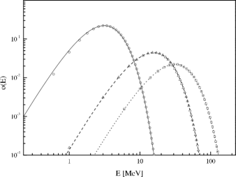
Figure 5: Numerically computed points of the neutrino spectrum (symbols) and the fit (lines). Curves represent spectra for $kT=1,5,10$ MeV. Even in in the worst case considered, $kT=1$ MeV ($\circ$), fit (54) is particularly good.

In more difficult cases, e.g. required for neutrinos from the pre-supernova core, where $kT\sim m_{e}\sim\mu$, one must use general expressions for neutrino energy moments, with wealth of analytical Blinnikov and Rudzskij (1989); Antia (1993) and numerical Aparicio (1998); Cloutman (1989) methods available for calculating Fermi-Dirac integrals. In the degenerate case differences between neutrino and antineutrino spectrum (and between $\nu_{e}$ and $\nu_{\mu,\tau}$ as well, cf. Fig. 4) must be taken into account. However, in typical situations they may be considered as a small perturbation to the average value.

If for some reasons exact results are required, the spectrum may be computed from (37) point-by-point as well.