RODEO: a new method for planet-disk interaction

In this paper we describe a new method for studying the hydrodynamical problem of a planet embedded in a gaseous disk. We use a finite volume method with an approximate Riemann solver (the Roe solver), together with a special way to integrate the source terms. This new source term integration scheme sheds new light on the Coriolis instability, and we show that our method does not suffer from this instability.The first results on flow structure and gap formation are presented, as well as accretion and migration rates. For $M_{\mathrm{p}}$$<0.1$ $\mathrm{{M}_{J}}$ and $M_{\mathrm{p}}$$>1.0$ $\mathrm{{M}_{J}}$ ($\mathrm{{M}_{J}}$ = Jupiter’s mass) the accretion rates do not depend sensitively on numerical parameters, and we find that within the disk’s lifetime a planet can grow to $3-4$ $\mathrm{{M}_{J}}$. In between these two limits numerics play a major role, leading to differences of more than $50\%$ for different numerical parameters. Migration rates are not affected by numerics at all as long as the mass inside the Roche lobe is not considered. We can reproduce the Type I and Type II migration for low-mass and high-mass planets, respectively, and the fastest moving planet of $0.1$ $\mathrm{{M}_{J}}$ has a migration time of only $2.0\leavevmode\nobreak\ 10^{4}$ yr.

1 Introduction

It is now generally believed that planets are formed out of the same nebula as their parent star. When this cloud of gas collapses into a protostar, conservation of angular momentum leads to the formation of an accretion disk around the star. These disks are indeed observed around T-Tauri stars (Beckwith & Sargent 1996), and it is within these disks that planet formation should take place.

In standard theory, terrestrial planets as well as the rocky cores of gas giant planets arise slowly from collisions of dust particles. When a protoplanet reaches a certain critical mass ($\approx 15$ $\rm M_{\oplus}$), it can no longer sustain a hydrostatic atmosphere, and dynamical accretion sets in. Eventually, this accretion process forms a gaseous envelope around the core, of a mass comparable to Jupiter. This scenario is known as the ’core accretion model’.

Recently, Boss (1997) revisited a model originally proposed by Cameron (1978), the ’core collapse scenario’, in which a giant planet is formed in much the same way as a star through a gravitational instability in the disk. However, Rafikov (2005) pointed out several problems with this scenario, and it is yet undecided which of these two scenarios is correct. In both cases we end up with a newly formed giant planet still embedded in the protoplanetary disk. It is this interesting stage of planet formation that we focus on in this paper.

The disk and the planet interact gravitationally with each other. The planet perturbs the disk through tidal forces, breaking its axisymmetry and, if the planet is massive enough, opens up a gap in the disk (Lin & Papaloizou 1993). The perturbed disk in its turn exerts a torque on the planet, leading possibly to orbital migration (Goldreich & Tremaine 1980). Inward migration is generally believed to be the mechanism responsible for creating ’Hot Jupiters’: giant planets, comparable to Jupiter, with very small semi-major axes ($<0.1$ AU).

The process of gap formation raises two interesting questions. First: does the presence of the gap prevent further gas accretion? If it does, this puts serious constraints on the maximum planet mass that can be reached. Secondly: how is the orbital evolution of the planet affected by the gap? If all planets move inward on much shorter time scales than the typical lifetime of the disk, how come we still have Jupiter in our Solar system at $5.2$ AU?

The accretion issue has been investigated in detail numerically by Kley (1999) and by Lubow et al. (1999), and they find that accretion can continue through the gap, allowing more massive planets to be formed. Migration has been investigated both analytically (Goldreich & Tremaine 1980; Lin & Papaloizou 1986), recently by Rafikov (2002), and numerically by Nelson et al. (2000) and Kley (2000), and it seems that migration is always inward, allowing for Hot Jupiters but not for ‘Cold’ Jupiters. Recently Masset & Papaloizou (2003) and Artymowicz (2004) showed that there exists a runaway regime in which the orbital radius of the planet evolves on very short timescales, with possible outward migration.

However, the problem is complicated analytically, and hard to do numerically as well. A nice illustration of this is given by Kley (1998), who showed that the use of a corotating coordinate frame can lead to non-physical evolution in some numerical codes. It therefore seems appropriate to introduce a numerical method which is new in this field of research, and which should handle rotating coordinate frames and the effects of gravity in a better way. We use a finite-volume method based on an approximate Riemann solver for arbitrary coordinate frames, which can is specifically aimed to treat discontinuities in the flow correctly. Also, the numerical scheme is conservative, meaning that the method conserves mass, momentum and angular momentum up to second order.

In this paper, we aim to give a full description of RODEO (ROe solver for Disk-Embedded Objects), to show some differences in the gas flow in the disk and to present results on accretion and migration rates. The focus will be more on numerical effects than on physical effects, i.e. we do not consider different disk structures or different magnitudes of an anomalous viscosity as was done by Bryden et al. (1999) and Kley (1999). Instead, we consider the effect of various numerical parameters to assess their importance regarding gap formation, accretion and migration rates.

We focus on the two-dimensional, vertically integrated problem, which is formally only correct for planets for which the Roche lobe is larger than the disk scale height. For our disk, this comes down to $M_{\mathrm{p}}$$>$ $\mathrm{{M}_{J}}$. However, because two-dimensional simulations are far less expensive in terms of computing time than three-dimensional simulations this allows us to do a detailed numerical study and compare our findings to previous two-dimensional results.

We start in Sect. 2 by describing the physical model that was used. Next, we focus on the numerical method in some detail in Sect. 3. In Sect. 4 we show the results of some test problems and in Sect. 5 we give the initial and the boundary conditions. We give our results on gap formation, accretion and migration in Sects. 6, 7 and 8. Section 9 is reserved for a short summary and the conclusions.

2 Physical Model

2.1 Basic equations

Protoplanetary disks are fairly thin, i.e. the ratio of the vertical thickness $H$ and the radial distance from the center $r$ is smaller than unity. Typically $H/r=0.05$. We can therefore vertically integrate the hydrodynamical equations, and work with vertically averaged state variables. We will use cylindrical coordinates $(r,\phi)$, with the central star of $1$ $\mathrm{M_{\odot}}$ located at $r=0$.

The flow of the gas is determined by the Euler equations, which express conservation of mass, momentum in all spatial directions, and energy. These equations can be written in a simple form:

$$\frac{\partial\@vec{W}}{\partial t}+\frac{\partial\@vec{F}}{\partial r}+\frac{\partial\@vec{G}}{\partial\phi}=\@vec{S},$$ (1)

where $\@vec{W}$ is called the state, $\@vec{F}$ and $\@vec{G}$ are the radial and the polar flux, respectively, and $\@vec{S}$ is the source term. The state consists of the conserved quantities, and Eq. (1) expresses the fact that any change in time of the state in a specific volume is due to flow across the boundary of the volume (the flux terms) or due to a source inside the volume (the source term). We will omit the energy equation for now, because we will work with a simple (isothermal) equation of state, which does not require an energy equation. The method still includes the energy equation as an option, however, and this way we have another way of simulating isothermal flow: a run with a very low adiabatic exponent $\Gamma$, as was done for example in Nelson & Benz (2003). We will present the method only for the isothermal equations; for the full method including the energy equation we refer to Eulderink & Mellema (1995).

In cylindrical coordinates, the vectors $\@vec{W}$, $\@vec{F}$, $\@vec{G}$ and $\@vec{S}$ can be written in the following form:

$$\@vec{W}=r(\Sigma,\leavevmode\nobreak\ \Sigma v_{\mathrm{r}},\leavevmode\nobreak\ \Sigma v_{\mathrm{\phi}})$$ (2)

$$\@vec{F}=r(\Sigma v_{\mathrm{r}},\leavevmode\nobreak\ \Sigma v_{\mathrm{r}}^{2}+p,\leavevmode\nobreak\ \Sigma v_{\mathrm{r}}v_{\mathrm{\phi}})$$ (3)

$$\@vec{G}=r(\Sigma v_{\mathrm{\phi}},\leavevmode\nobreak\ \Sigma v_{\mathrm{r}}v_{\mathrm{\phi}},\leavevmode\nobreak\ \Sigma v_{\mathrm{\phi}}^{2}+p/r^{2})$$ (4)

$$\@vec{S}=\left(\begin{array}[]{c}0\\ \Sigma r^{2}(v_{\phi}+\Omega)^{2}-\Sigma r\frac{\partial{\Phi}}{\partial{r}}+p\\ -2\Sigma v_{\mathrm{r}}(\Omega+v_{\phi})-\frac{\Sigma}{r}\frac{\partial{\Phi}}{\partial{\phi}}\end{array}\right)$$ (8)

The symbols used are listed in Table 1.

Table 1: Definition of symbols

$\begin{array}[]{ll}\hline\cr r&$radial coordinate$\\ \phi&$azimuthal coordinate$\\ \Sigma&$surface density$\\ v_{\mathrm{r}}&$radial velocity$\\ v_{\phi}&$angular velocity in the corotating frame$\\ p&$vertically integrated pressure$\\ \Phi&$gravitational potential$\\ \Omega&$angular velocity coordinate system$\\ r_{\mathrm{p}}&$orbital radius of the planet$\\ P&$orbital period of the planet$\\ \end{array}$

Note that in this form there are no derivatives of dependent variables in the source term, keeping $\@vec{S}$ finite even in the presence of discontinuities. Also, there are no viscous terms present, because we deal with viscosity in a separate way (see Sect. 2.3).

The gravitational potential contains terms due to the central star and due to the direct and indirect influence of the planet:

$$\Phi(r,\phi)=-\frac{\rm{GM_{\odot}}}{r}-\frac{{\rm{G}}M_{\rm{p}}}{r_{2}}+\frac{{\rm G}M_{\rm{p}}}{r_{\mathrm{p}}^{2}}r\cos(\phi-\phi_{\mathrm{p}})$$ (9)

Here $r_{2}=|r-r_{\mathrm{p}}|$ denotes the distance to the planet. Because this potential is singular at the position of the planet, and to account for the threedimensional structure of the disk, we use a smoothed version of $r_{2}$:

$$r_{2}=\sqrt{r^{2}+r_{\mathrm{p}}^{2}-2r\leavevmode\nobreak\ r_{\mathrm{p}}\leavevmode\nobreak\ \cos(\phi-\phi_{\mathrm{p}})+\epsilon^{2}}\\$$

The smoothing parameter $\epsilon$ is taken to be a certain fraction of the Roche lobe of the planet:

$$\epsilon=b\leavevmode\nobreak\ \mathrm{R_{R}}=b\leavevmode\nobreak\ r_{\mathrm{p}}\leavevmode\nobreak\ \sqrt[3]{\frac{M_{\mathrm{p}}}{3\mathrm{M_{\odot}}}}$$ (10)

Throughout this paper we have used $b=0.2$. The results do not depend much on its value, as long as $b<1$. The indirect term in the potential (the last term on the right-hand side in Eq. 9) arises due to the fact that a coordinate system centered on the central star is not an inertial frame, because the star feels the gravitational pull of the planet. A similar (small) term for the disk is omitted for simplicity.

2.2 Equation of state

Equation (1) needs to be complemented by an equation of state. We assume an isothermal equation of state:

$$p=c_{\mathrm{s}}^{2}\Sigma$$ (11)

This choice is based on the assumption that the gas is able to radiate away all its excess energy very efficiently. In vertical hydrostatic equilibrium, the isothermal sound speed $c_{\mathrm{s}}$ is given by:

$$c_{\mathrm{s}}=\frac{H}{r}\sqrt{\frac{\mathrm{G\leavevmode\nobreak\ M_{\odot}}}{r}},$$ (12)

2.3 Viscosity

The nature of the viscosity in accretion disks was unknown for a long time. Currently, the Magneto-Rotational Instability (MRI) is the best candidate for providing a turbulent viscosity (Balbus & Hawley 1990). In regions where the ionisation fraction in the disk is high enough to sustain the MRI one would need to do Magneto-Hydrodynamics (MHD) to study planet-disk interaction, as was done in Nelson & Papaloizou (2003). MHD simulations are very expensive however, and it is not yet clear if the MRI operates throughout the disk. In so-called dead-zones (Gammie 1996) there may be no turbulent viscosity at all. However, in order to compare our results to previous studies we include an anomalous turbulent viscosity in our models.

Viscosity comes in as two extra source terms for the momentum, one in the radial and one in the azimuthal direction. We deal with these source terms separately in the numerical method (see Sect. 3).

The form of these source terms can be found for example in D’Angelo et al. (2002):

$$f_{\mathrm{r}} = \frac{1}{r}\frac{\partial(r\mathcal{S}_{\mathrm{rr}})}{\partial r}+\frac{1}{r}\frac{\partial(\mathcal{S}_{\mathrm{r\phi}})}{\partial\phi}-\frac{\mathcal{S}_{\phi\phi}}{r}$$ (13)

$$f_{\phi} = \frac{1}{r}\frac{\partial(r^{2}\mathcal{S}_{\mathrm{r\phi}})}{\partial r}+\frac{\partial(\mathcal{S}_{\phi\phi})}{\partial\phi}$$ (14)

where the components of the viscous stress tensor $\mathcal{S}$ are:

$$\mathcal{S}_{\mathrm{rr}} = 2\nu\Sigma\left(\frac{\partial v_{\mathrm{r}}}{\partial r}-\frac{1}{3}\nabla\cdot\@vec{v}\right)$$ (15)

$$\mathcal{S}_{\phi\phi} = 2\nu\Sigma\left(\frac{\partial v_{\phi}}{\partial\phi}+\frac{v_{\mathrm{r}}}{r}-\frac{1}{3}\nabla\cdot\@vec{v}\right)$$ (16)

$$\mathcal{S}_{\mathrm{r\phi}} = \nu\Sigma\left(\frac{1}{r}\frac{\partial v_{\mathrm{r}}}{\partial\phi}+r\frac{\partial v_{\phi}}{\partial r}\right)$$ (17)

$$\nabla\cdot\@vec{v} = \frac{1}{r}\frac{\partial(rv_{\mathrm{r}})}{\partial r}+\frac{\partial v_{\phi}}{\partial\phi}$$ (18)

We can either use an $\alpha$-prescription for the viscosity parameter $\nu$ (Shakura & Sunyaev 1973):

$$\nu=\alpha c_{\mathrm{s}}H$$ (19)

or we can take $\nu$ constant throughout the disk. Note that for the $\alpha$-disk with constant aspect ratio $H/r$, $\nu\propto\sqrt{r}$, leading to enhanced viscosity in the outer disk.

3 Numerical Method

We can integrate Eq. (1) over the finite volume of a grid cell to obtain:

$$\frac{1}{\Delta t\Delta r\Delta\phi}\leavevmode\nobreak\ (\int dr\int d\phi\leavevmode\nobreak\ (\@vec{W}^{n+1}-\@vec{W}^{n})+$$

$$\int dt\int d\phi\leavevmode\nobreak\ (\@vec{F}_{i+1/2,j}-\@vec{F}_{i-1/2,j})+$$

$$\int dt\int dr\leavevmode\nobreak\ (\@vec{G}_{i,j+1/2}-\@vec{G}_{i,j-1/2})-$$

$$\int dt\int dr\int d\phi\leavevmode\nobreak\ \@vec{S})=0$$ (20)

Here $A^{n}_{i,j}$ means the physical quantity $A$, evaluated at time index $n$, at coordinates $(i,j)$. The volume term ($r^{2}\sin\theta$ for spherical coordinates, $r$ for cylindrical coordinates) of the grid cell is already present in $\@vec{W}$, $\@vec{F}$ and $\@vec{S}$. A second order accurate integration scheme for this equation is:

$$\frac{1}{\Delta t}(\langle\@vec{W}\rangle^{n+1}-\langle\@vec{W}\rangle^{n})+$$

$$\frac{1}{\Delta r}\leavevmode\nobreak\ (\@vec{F}^{n+1/2}_{i+1/2,j}-\@vec{F}^{n+1/2}_{i-1/2,j})+$$

$$\frac{1}{\Delta\phi}\leavevmode\nobreak\ (\@vec{G}^{n+1/2}_{i,j+1/2}-\@vec{G}^{n+1/2}_{i,j-1/2})-$$

$$\@vec{S}^{n+1/2}_{i,j}=0$$ (21)

where $\langle\rangle$ denotes arithmetic mean. A numerical scheme like this is called conservative because the conserved quantities are indeed conserved by the numerical method: what goes into one cell must come out of another.

We will use Eq. (21) to find an update for the state. What is left to be done is to find expressions for the interface fluxes (Sect. 3.1) and to account for the source terms (Sect. 3.2).

3.1 Roe solver

First, we use the technique of dimensional splitting to obtain the two one-dimensional equations

$$\frac{\partial{\@vec{W}}}{\partial{t}}+\frac{\partial{\@vec{F}}}{\partial{r}}=\@vec{X}$$

$$\frac{\partial{\@vec{W}}}{\partial{t}}+\frac{\partial{\@vec{G}}}{\partial{\phi}}=\@vec{Y}$$ (22)

The order in which these equations are solved is alternated to avoid systematic numerical effects (Strang 1968). We have the freedom of choosing the splitting of the source term any suitable way. We discuss a special way in Sect. 3.2.

From now on, we focus on the radial direction; the azimuthal integration is done in a similar way. We split Eq. (3.1) once more to obtain an equation without source terms, and solve this equation with a method originally proposed by Roe (1981), and extended by Eulderink & Mellema (1995) to a general relativistic method. The non-relativistic limit of this method yields a solver for the Euler equations in arbitrary coordinates.

3.1.1 Characteristics

Given the state (or the flux) immediately left and right of an interface of two grid cells, the Roe solver computes the resulting interface flux by solving:

$$\frac{\partial\@vec{W}}{\partial{t}}+\mathcal{A}(\@vec{W})\frac{\partial\@vec{W}}{\partial r}=0$$ (23)

where $\mathcal{A}(\@vec{W})=\partial\@vec{F}/\partial\@vec{W}$ is the Jacobian matrix. Roe’s central idea is to approximate $\mathcal{A}(\@vec{W})$ by a constant matrix $\tilde{\mathcal{A}}$. Since the Euler equations are hyperbolic, this matrix $\tilde{\mathcal{A}}$ has eigenvectors $\@vec{e}_{k}$ and corresponding eigenvalues $\lambda_{k}$. These can be used to diagonalize $\tilde{\mathcal{A}}$:

$$\mathcal{Q}^{-1}\leavevmode\nobreak\ \tilde{\mathcal{A}}\leavevmode\nobreak\ \mathcal{Q}=\mathcal{D}$$ (24)

where $\mathcal{Q}$ is the matrix with right eigenvectors of $\tilde{\mathcal{A}}$. Now we can cast Eq. (23) into characteristic form:

$$\frac{\partial\@vec{C}}{\partial t}+\mathcal{D}\frac{\partial\@vec{C}}{\partial r}=0$$ (25)

where $\@vec{C}$ is the vector of characteristic variables, defined by

$$d\@vec{C}=\mathcal{Q}^{-1}\leavevmode\nobreak\ d\@vec{W}$$ (26)

and $\mathcal{D}$ is the diagonal matrix with eigenvalues of $\tilde{\mathcal{A}}$. From (25) it is easy to see that $d\@vec{C}=0$ along the path $\@vec{r}=\mathcal{D}\@vec{t}$. These paths are called characteristics, and are essential in the study of hyperbolic differential equations. Discontinuities (shocks) travel along characteristics, and the domains of influence and dependence are bounded by the characteristics.

We can integrate Eq. (25) to find a relation between the state and the characteristic variables:

$$\@vec{W}=\mathcal{Q}\@vec{C}=\sum_{k}a_{k}\@vec{e}_{k}$$ (27)

where $a_{k}$ is the k-th characteristic variable. As the $a_{k}$ are used to project the state on the eigenvectors of $\tilde{\mathcal{A}}$, they are called projection coefficients.

We can use the projection coefficients for calculating the interface flux, because we know that they are constant along characteristics. If we can figure out from which point in space the characteristics that cross the interface originate at the current time, we can just calculate the projection coefficients at that point in space and use Eq. (27) to find the state at the interface.

The interface flux is related to the interface state by:

$$\@vec{F}=\tilde{\mathcal{A}}\@vec{W}=\tilde{\mathcal{A}}\mathcal{Q}\@vec{C}=\mathcal{Q}\mathcal{D}\@vec{C}=\sum_{k}b_{k}\@vec{e}_{k}$$ (28)

where $b_{k}=\lambda_{k}a_{k}$. We present the exact expressions for the eigenvalues, eigenvectors and projection coefficients in Appendix A.

We can project the flux difference at the interface we are considering on the eigenvectors of $\tilde{\mathcal{A}}$:

$$\@vec{F}_{R}-\@vec{F}_{L}=\sum b_{k}\@vec{e}_{k}$$ (29)

where $\@vec{F}_{R}$ and $\@vec{F}_{L}$ are the fluxes immediately right and left of the interface, respectively. Then the first order interface flux is approximated by:

$$\@vec{F}^{n+1/2}_{i+1/2}=\frac{1}{2}(\@vec{F}_{L}+\@vec{F}_{R})-\frac{1}{2}\sum\sigma_{k}b_{k}\@vec{e}_{k}$$ (30)

where $\sigma_{k}=\rm{sign}(\lambda_{k})$.

3.1.2 Flux limiter

The first order expression for the flux, Eq. (30), assumes a jump in the projection coefficients. That is: depending on the sign of the eigenvalue $\lambda_{k}$, we use the $b_{k}$ corresponding to either the left or the right state. This procedure is correct if there is a shock right at that interface, so the state makes a jump there. In regions of smooth flow however, linear interpolation between the different $b_{k}$ seems to be a better approach. To switch between the two kinds of interpolation a flux limiter $\psi$ is used. We follow the suggestion by Roe (1985), in which one uses the ratio of the state difference at the interface $a_{0}=[a_{k}]_{i+1/2}$ to the upwind state difference:

$$a_{u}=\left\{\begin{array}[]{ll}(a_{k})_{i-1/2}&\mbox{if $\lambda_{k}\geq 0$};\\ (a_{k})_{i+3/2}&\mbox{if $\lambda_{k}<0$}\end{array}\right.$$

Let

$$\psi(a_{0},a_{u})=\max(0,\min(pa_{u},\max(a_{0},\min(a_{u},pa_{0}))))+$$

$$\min(0,\max(pa_{u},\min(a_{0},\max(a_{u},pa_{0}))))$$ (31)

This form of the flux limiter allows us to tune the way the method deals with sharp discontinuities through the parameter $p$. When $p=2$, for example, the flux limiter is called ’Superbee’. This limiter tends to create very sharp shocks, but tends to steepen shallow gradients, leading to numerical problems such as under- and overshoots. For $p=1$ the limiter is called ’minmod’, which is more diffusive. To get the best of both worlds (sharp shocks but no under- or overshoots), we set $p=1.5$ in all simulations.

With this flux limiter, the second order interface flux becomes:

$$\@vec{F}^{n+1/2}_{i+1/2}=\frac{1}{2}(\@vec{F}_{L}+\@vec{F}_{R})-\frac{1}{2}\sum(\sigma_{k}a_{k}-(\sigma_{k}-\nu_{k})\psi_{k})\lambda_{k}\@vec{e}_{k}$$ (32)

where $\nu_{k}=\lambda_{k}\Delta t/\Delta r$, the coefficient needed for linear interpolation. When $\psi_{k}=0$ (shock), Eq. (30) is retrieved, while for $\psi_{k}=1$ (smooth flow) the $\sigma_{k}$ in Eq. (30) is replaced by $\nu_{k}$ and we interpolate linearly between the projection coefficients.

3.2 Stationary Extrapolation

The usual way for dealing with source terms is to split Eq. 22 once more to end up with an ordinary differential equation for the state:

$$\frac{\partial\@vec{W}}{\partial t}=\@vec{X},\quad\frac{\partial\@vec{F}}{\partial r}=0$$ (33)

thereby assuming that the flux is constant in space. The ordinary differential equation can be solved with any second-order integration scheme to yield a second-order update for the state.

However, it is also possible to take the opposite approach:

$$\frac{\partial\@vec{W}}{\partial t}=0,\quad\frac{\partial\@vec{F}}{\partial r}=\@vec{X}$$ (34)

This is a method we call stationary extrapolation, because it assumes a stationary state within one grid cell. This equation is more difficult to solve, but it has certain advantages:

• The Roe solver solves a Riemann problem at the interface, a configuration with two stationary states separated by a discontinuity. Using actual stationary states on either side of the interface ensures that the Roe solver deals with a genuine Riemann problem.

• Physical stationary states are recognized. When the actual states are stationary, the Roe solver will produce no (unwanted) numerical evolution of these states. This property is related to the numerical instability found by Kley (1998) concerning the Coriolis force. We will see below that a scheme using stationary extrapolation does not suffer from this instability.

If we split the source terms appropriately:

$$\@vec{X}=\left(\begin{array}[]{c}0\\ \Sigma r^{2}(v_{\phi}+\Omega)^{2}-\Sigma r\frac{\partial\Phi}{\partial r}+p\\ -2\Sigma v_{\rm{r}}(\Omega+v_{\phi})\end{array}\right)$$ (35)

$$\@vec{Y}=\left(\begin{array}[]{c}0\\ 0\\ -\frac{\Sigma}{r}\frac{\partial\Phi}{\partial\phi}\end{array}\right)$$ (36)

the integrations can be done analytically (Eulderink & Mellema 1995). For isothermal, stationary flow in the radial direction Eq 34 can be rewritten:

$$\frac{\partial}{\partial r}\left(\begin{array}[]{c}r\Sigma v_{\rm r}\\ \frac{1}{2}(v_{\rm r}^{2}+r^{2}v_{\phi}^{2})+\Phi+c^{2}\log(\Sigma)\\ r^{2}(v_{\phi}+\Omega)\end{array}\right)=0$$ (37)

That is: the mass flux, the Bernouilli constant and the specific angular momentum are invariant. From these invariants the state at a cell interface can be computed from the state at the cell center. However, this procedure is computationally expensive, therefore it is feasible to adopt a first order approximation to calculate the interface fluxes:

$$\@vec{F}_{i-1/2,R}=\@vec{F}_{i}-\frac{1}{2}\Delta r\@vec{X}_{i}$$

$$\@vec{F}_{i-1/2,L}=\@vec{F}_{i-1}+\frac{1}{2}\Delta r\@vec{X}_{i-1}$$ (38)

This procedure can conserve stationary states up to second order (Mellema et al. 1991). However, Kley (1998) showed that the angular momentum in disk simulations deserves special attention. We illustrate this with a simple example. Consider the radial transport of angular momentum:

$$\frac{\partial}{\partial t}(r\Sigma v_{\phi})+\frac{\partial}{\partial r}(r\Sigma v_{r}v_{\phi})=-2\Sigma v_{r}(v_{\phi}+\Omega)$$ (39)

For stationary radial flow the mass flux and the specific angular momentum are constant: $r\Sigma v_{r}=D$ and $r^{2}(v_{\phi}+\Omega)=L$. For simplicity we assume here that $D$ is constant for the whole computational domain. Consider the interface between cells $i$ and $i-1$. Stationary extrapolation from the cell centers to the interface $i-1/2$ leads to the fluxes

$$F_{L}=D(\frac{L_{i-1}}{r_{i-1/2}^{2}}-\Omega)$$ (40)

$$F_{R}=D(\frac{L_{i}}{r_{i-1/2}^{2}}-\Omega)$$ (41)

With $v_{r}>0$, the first order interface flux produced by the Roe solver is $F_{i-1/2}=F_{L}$. Therefore

$$L_{i-1/2}=r_{i-1/2}^{2}(F_{L}/D+\Omega)=L_{i-1}$$ (42)

Stationary extrapolation from the interface back to the cell center $i$ gives the final flux coming from the left for cell $i$:

$$F_{L,i}=D(\frac{L_{i-1}}{r_{i}^{2}}-\Omega)$$ (43)

From the same analysis for interface $i+1/2$ we find the flux going to the right for cell $i$:

$$F_{R,i}=D(\frac{L_{i}}{r_{i}^{2}}-\Omega)$$ (44)

The first order update for the state is:

$$\Delta(r\Sigma v_{\phi})=\frac{\Delta t}{\Delta r}(F_{L,i}-F_{R,i})=\frac{\Delta t}{\Delta r}\frac{D}{r_{i}^{2}}(L_{i-1}-L_{i})$$ (45)

The change in angular momentum $J=r^{2}\Sigma(v_{\phi}+\Omega)$ due to this update is given by:

$$\Delta J=\frac{\Delta t}{\Delta r}\frac{D}{r_{i}}(L_{i-1}-L_{i})$$ (46)

It is easy to see that the conservative formulation of Kley (1998):

$$\frac{\partial}{\partial t}(r\Sigma L)+\frac{\partial}{\partial r}(r\Sigma v_{r}L)=0$$ (47)

leads to the same change in angular momentum. This shows that this new method does not suffer from the numerical instability due to the explicit treatment of the Coriolis force that was noted by Kley (1998). Note however that this does not hold for the approximate extrapolation of Eq. 38. Therefore we always use the exact extrapolation for the specific angular momentum, while keeping the method of approximate extrapolation to deal with the other source terms. This way we do not need to do the computationally intensive full stationary extrapolation, while keeping angular momentum nicely conserved.

Stationary extrapolation therefore provides a different point of view on the Coriolis instability: the failure of numerical hydrodynamic schemes to properly conserve angular momentum can be traced back to the failure to recognize stationary states. Rewriting the angular momentum equation as done by Kley (1998) is a way to solve this problem, but it only deals with the Coriolis source term while similar problems may exist due to the other source terms as well. Therefore we feel that it is a good idea to integrate all source terms using stationary extrapolation.

One disadvantage of stationary extrapolation is that it is not known a-priori if the assumption of stationary flow is valid. This is especially important when the source terms are large, in our case very close to the planet. When dealing with more massive planets ($>0.5$ $\mathrm{{M}_{J}}$) the assumption of stationary flow along the coordinate axes breaks down, leading to numerical instabilities. A physical explanation is that the gas in this case will try to orbit the planet, perhaps forming a Keplerian disk, rather than to orbit the star. The flow is still semi-stationary, but only in a cylindrical coordinate frame centered on the planet, and this flow is at some points even orthogonal to the stationary flow in the frame of the star. Therefore, it seems appropriate to treat these larger source terms as external (see section 3.2.1). This transition from stationary to non-stationary extrapolation is applied smoothly at a typical distance $R_{\rm R}$ from the planet with a $\sin^{2}$ ramp.

3.2.1 External source terms

The stationary extrapolation deals with the geometrical source terms (including gravity, which is merely a geometrical effect in general relativity). Any other source term which we will call $\@vec{Z}$ is better integrated using Eq. (33):

$$\textbf{W}^{n+1}=\textbf{W}^{n}+\Delta t\textbf{Z}$$ (48)

In our case, $\@vec{Z}$ consists of the viscous source terms. The derivatives in these terms are calculated using a finite-difference method, and the resulting source is fed into Eq. (48).

3.3 Adaptive Mesh Refinement

Resolution is always an issue in numerical hydrodynamics, and a compromise has to be found between resolution and computational cost. Adaptive Mesh Refinement (AMR) is a very economic way of refining your grid where the highest resolution is needed, whereas keeping large parts of the grid at low resolution.

We have implemented the PARAMESH algorithm (MacNeice et al. 2000) to be able to resolve the region near the planet accurately. Usually the refinement criterium is taken to be the second derivative of the density, but we can also predefine the region that has to be refined. When running in this mode, and switching off additional refining and derefining, the algorithm works like the nested grid technique of D’Angelo et al. (2002). However, since our grid can be fully adaptive it is suited to let the planet migrate through the disk while keeping a high resulution near the planet. This will be the subject of a future paper.

We use linear interpolation to communicate boundary cells between the different levels of refinement. The implementation of the monotonised harmonic mean (van Leer 1977) used by D’Angelo et al. (2002) made no significant difference. For every boundary between different levels we reset the flux into the lower level in order to conserve mass and momentum across the boundary.

3.4 Accretion

We follow D’Angelo et al. (2002) in modeling the accretion by taking away some fraction of the density within a distance of $r_{\mathrm{acc}}$ of the planet. Basically, the density is reduced with a factor

$$1-f\leavevmode\nobreak\ \Delta t,$$ (49)

where $\Delta t$ is the magnitude of the time step. The two parameters that determine the accretion rate are $r_{\mathrm{acc}}$ and $f$, where $f$ is taken to be twice its value in the inner half of $r_{\mathrm{acc}}$. The mass taken out is monitored, assuming it has been accreted onto the planet, but without changing the dynamical mass of the planet.

Equation 49 can be seen as a first order approximation to the solution of the differential equation

$$\frac{d\rho}{dt}=-\frac{\rho}{\tau_{\rm acc}}$$ (50)

with the solution

$$\rho(t+\Delta t)=\rho(t)e^{-\Delta t/\tau_{\rm acc}}\approx\rho(t)\left(1-\Delta t/\tau_{\rm{acc}}\right)$$ (51)

From this equation we see that the typical time scale $\tau_{\rm{acc}}$ for emptying the accretion region is $f^{-1}$.

Figure 1: The evolution of the axisymmetric gas ring, initially located at x=1, shown at $\tau=0.05$, and after 50 and 100 orbits. For the last two the numerical results are also plotted (diamonds and triangles, respectively.

4 Test Problems

We tested the RODEO method against several hydrodynamical test problems. First of all, the standard Sod shocktube (Sod 1978), in one and in two dimensions. For the two-dimensional problem, we have placed the initial discontinuity diagonal along the grid, making it a genuine two-dimensional problem. The analytic solution was nicely recovered, except at the boundaries where some reflections were seen.

A more complicated test is the windtunnel with step (Woodward & Colella 1984), which was previously used as a testproblem by Mellema et al. (1991) using the same method. The results agreed very well. Note that both tests do use an energy equation.

4.1 Viscous ring spreading

To test the implementation of the viscous terms, we set up an axisymmetric ring of gas in Keplerian rotation about a central object. If we neglect pressure forces, the evolution of the surface density, which initially is a delta function, is given by Pringle (1981):

$$\Sigma(r,t)=\frac{1}{\pi r_{0}^{2}\tau x^{1/4}}e^{-\frac{1+x^{2}}{\tau}}\leavevmode\nobreak\ I_{1/4}\left(\frac{2x}{\tau}\right)$$ (52)

where x denotes the normalized radial coordinate $r/r_{0}$, with the ring initially located at $r=r_{0}$, and $\tau$ denotes the dimensionless time ($\tau=t/t_{v}$) in units of the viscous spreading time $t_{v}=r_{0}^{2}/12\nu$. $I_{1/4}$ denotes the Bessel function of the first kind of fractional order $1/4$.

As the analytical solution neglects any forces due to a pressure gradient, we have to make sure that we set the temperature to a very low value, or else pressure waves will dominate the pattern. We have used the same resolution as for simulations with the planet, and with a viscosity parameter $\alpha=0.004$ at $x=1$, comparable to the value used in the disk-planet simulations. We have placed the ring in the middle of the computational domain of $x\in[0.27,1,73]$, with $\tau=0.05$ initially because we cannot model a delta function numerically.

We have also performed a test run of this problem using $\alpha=0$ to check for numerical viscosity, and it turned out that this (unwanted) numerical diffusion was very much lower than any physical viscosity. at a low resolution of 128x384. Note that this also shows that we can maintain a stable disk in Keplerian rotation. This is a nice result, showing that our conservative scheme conserves angular momentum very well.

Figure 1 shows the results for $\alpha=0.004$. It is clear that the numerical solution agrees very well with Eq. (52), indicating that the implementation of the viscosity works. Only at the boundaries there are minor deviations from the analytical solution.

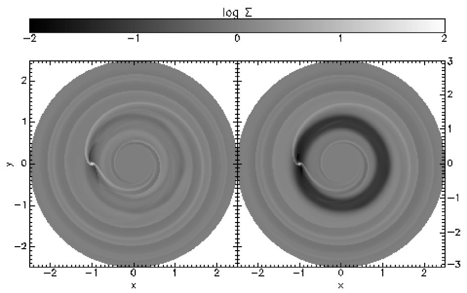
Figure 2: Greyscale plot in $(x,y)$ after $10$ orbits (left panel) and after $200$ orbits (right panel) of a 1 $\mathrm{{M}_{J}}$ planet.

5 Model design

Throughout we use non-dimensional units. The unit of distance is the orbital radius of the planet, and the unit of time is the inverse orbital frequency. Note that this differs by a factor $2\pi$ from the orbital period of the planet.

5.1 Initial Conditions

The base resolution in all our simulations is $(n_{\mathrm{r}},n_{\mathrm{\phi}})=(256,768)$, which leads to square cells near the position of the planet. We set $h=H/r=0.05$, which determines the temperature through Eq. 12. We take a constant initial surface density. Because we do not consider the self-gravity of the disk the density can be given in any desirable unit, and we normalize it to $1$ at the planet’s position. We set the radial velocity to zero, although another possibility is to take an exact $\alpha$-disk initially. The initial angular velocity is set to the value for a Keplerian disk, with a small correction for the pressure force.

We take a constant kinematic viscosity $\nu=10^{-5}$, corresponding to $\alpha=0.004$ at the location of the planet. We put in a planet at location $(r,\phi)=(1,\pi)$. This planet can be allowed to accrete matter (without changing its dynamical mass).

5.2 Boundary conditions

The inner and the outer boundary are located at $0.4$ and $2.5$, respectively. Imposing proper boundary conditions is not trivial, because waves are continuously hitting both edges of the grid, changing the sign of the radial velocity. A standard outflow boundary assumes that the velocity is always directed outward, and in combination with outgoing waves this leads to instabilities near the inner radius of the disk. A reflecting boundary, on the other hand, will lead to reflected waves traveling into the computational domain, which interact with the outgoing waves, destroying the flow structure.

Therefore we decided to take a non-reflecting boundary, following Godon (1996). This boundary treatment is based on characteristics, and as a result the implementation is particularly simple in our numerical scheme. The idea is to impose the boundary conditions on the characteristic variables, rather than on density, momentum or energy directly. Godon (1996) showed that this leads to a non-reflective boundary.

A ghost cell has to be updated according to incoming characteristics: when a characteristic leaves the last regular cell into the ghost cell, the corresponding characteristic variable of the ghost cell is updated accordingly. When a characteristic enters the ghost cell from outside the numerical domain, the characteristic variable is updated using the unperturbed (Keplerian) value. Using the Roe solver, this comes down to having two ghost cells: the outer one is never updated, so density and velocities remain at the initial values, and the inner one serves as the actual ghost cell. The latter is automatically updated by the Roe solver using characteristic variables, thereby following the suggestion by Godon (1996).

It turns out that these boundary conditions work especially well with stationary extrapolation, because then the hydrodynamics part as well as the boundary prescription are dealing with small fluctuations over a stationary background state. When we switch to the ordinary integration of source terms of Eq. 33 this is no longer true. In this case small numerical artefacts can be seen near the boundaries.

Therefore, as an addition we can add a wave-damping mechanism (De Val-Borro et al. 2005) that operates in the regions $0.4<r<0.5$ and $2.1<r<2.5$. In these regions the state is relaxed to the initial (stationary) state on a time scale varying from infinity at $r=0.5$ and $r=2.1$ to 1 orbital period at the location of the boundary. Using this prescription, outgoing waves are damped gently as they approach the boundary of the computational domain.

Figure 3: Gap formation for a 1 $\mathrm{{M}_{J}}$ planet. Left panel: azimuthally averaged surface density for the case of exact stationary extrapolation. Right panel: azimuthally averaged surface density for the case of approximate extrapolation. The indicated times are in planetary orbits.

6 Gap Formation

Only massive planets are able to open gaps in gas disks. There are two criteria that have to be fullfilled: firstly, the torques arising due to the presence of the planet must be able to overcome the viscous torques, leading to a minimum mass of (Bryden et al. 1999):

$$M_{\mathrm{min,\nu}}=\frac{40\nu}{\Omega_{\mathrm{K}}r_{\mathrm{p}}^{2}}\mathrm{M_{\odot}}$$ (53)

Secondly, Lin & Papaloizou (1993) suggested that at a distance of $\mathrm{R_{R}}$ from the planet the planet’s gravity should be more important than pressure, which leads to another minimum mass for gap opening:

$$M_{\mathrm{min,h}}=3\leavevmode\nobreak\ h^{3}\leavevmode\nobreak\ \mathrm{M_{\odot}}$$ (54)

For our disk, with $\nu=10^{-5}$ and $h=0.05$ both criteria yield approximately the same minimum mass, namely $0.4$ $\mathrm{{M}_{J}}$. These criteria were shown to be valid within a factor of 2 in Bryden et al. (1999).

In our simulations, we found the density reduction factor near the orbit of the planet to be more than 100 for a 1 $\mathrm{{M}_{J}}$ planet, 10 for a $0.5$ $\mathrm{{M}_{J}}$ planet and 2 for a $0.1$ $\mathrm{{M}_{J}}$ planet. All factors were measured after $500$ orbits of the planet. In view of these results, we can confirm that both criteria give a good estimate of the minimum mass for gap opening. This seems to contradict recent results from Rafikov (2002), who found that it takes only a fraction of $M_{\mathrm{min,h}}$ to open a gap. This fraction depends on viscosity and disk mass, and it can be as low as $0.1$. However, in that analysis feedback from migration of the planet plays a role, while our planet remains fixed in the grid.

Figure 4: Azimuthally averaged density profile after $20$ orbits for different implementations of the source term integration: exact stationary extrapolation, approximate extrapolation and no stationary extrapolation.

Figure 2 (left panel) shows a greyscale plot of the surface density after $10$ orbits of a 1 $\mathrm{{M}_{J}}$ planet, and all the basic features in the flow are already visible. We can see two trailing spiral arms leaving the planet: the inner arm moves all the way down to the inner boundary, while the outer arm reaches to about $r=1.5$. Note also the secondary waves excited in the inner and in the outer disk.

All spiral waves are stationary in the corotating frame. For this run we did not take out any matter inside the Roche lobe, so the density reaches very high values near the planet.

The formation of the gap is quite a violent proces. There are structures visible in the corotating region and in the outer edge of the gap. The physical viscosity is able to damp these fluctuations, leading to a stable gap after 200 orbits (Fig. 2, right panel).

The left panel of Fig. 3 shows the azimuthally averaged surface density for the same run at different times. The gap that is formed is approximately $0.5\leavevmode\nobreak\ r_{\rm p}$ wide, with two density bumps on either side. After $100$ orbits the inner disk is starting to be accreted onto the central star. At all times the position of the planet is visible as a small spike at $r=1$.

The proces of gap formation is numerically challenging, as was already shown by Kley (1998). In the remainder of this section we study the formation of gaps as a function of numerical parameters.

6.1 Source term integration

First of all we focus on the integration of source terms. We consider four different methods. First of all our standard scheme, in which we solve for the angular momentum exactly, and integrate all other source terms using Eq. 38. Secondly, we have the approximate scheme, where all source terms are integrated using Eq. 38. Next, we consider the case of no stationary extrapolation at all (see Eq. 33), which is what ordinary Riemann-type schemes would use. Finally, we again integrate the angular momentum exactly, and all other source terms using Eq. 33. This mimics the fix found by Kley (1998), and we will refer to this scheme as hybrid, because it combines the two extremes of stationary extrapolation and no stationary extrapolation.

In Fig. 3 we show the formation of the gap for the exact stationary extrapolation (left panel) and the approximate stationary extrapolation (right panel). The difference between the two plots is quite dramatic. While both methods keep angular momentum conserved up to second order, approximate extrapolation leads to a much wider and deeper gap. After 200 orbits of the planet, even the region $1.5<r<2.1$ is participating in gap formation. From Fig. 3 it is clear that approximate extrapolation, while it preserves stationary states up to second order, is not the way to go in case of a strongly rotating fluid. Only the exact stationary extrapolation produces results comparable to other codes (see De Val-Borro et al. (2005)).

For these runs the wave damping boundary regions were employed to be able to compare to runs with no stationay extrapolation at all. The effect of the damping zones is clearly visible after 200 orbits, especially at the inner boundary.

Both models of Fig. 3 were also run in an inertial frame for comparison. For the case of exact extrapolation it made no difference at all, while only small changes were seen for approximate extrapolation. However, even in an inertial frame there is a Coriolis force term, see Eq. 8, so an inertial frame calculation is in this case not a valid check for the instability found by Kley (1998).

Figure 5: Azimuthally averaged density profile for a 1 $\mathrm{{M}_{J}}$ planet after $100$ orbits for different flux limiters: $p=1.5$ (standard value), $p=2.0$ and $p=1.0$ (see Eq. 31)

Figure 6: Azimuthally averaged density profile for a $0.1$ $\mathrm{{M}_{J}}$ planet after $200$ orbits in a non-viscous disk for different flux limiters: $p=1.5$ (standard value), $p=2.0$ and $p=1.0$ (see Eq. 31)

Figure 7: Accretion onto a 1 $\mathrm{{M}_{J}}$ planet. Left panel: total accreted mass in units of the initial disk mass. Right panel: accretion rate, in units of disk masses per orbit.

In Fig. 4 we compare the azimuthally averaged surface density profile for the four methods of source integration: standard, approximate, no stationary extrapolation at all, and the hybrid form. This figure shows that both the approximate extrapolation and the case of no stationary extrapolation overestimate the angular momentum transport, which leads to spurious gap widening. It is remarkable, however, that approximate extrapolation does the worst job, worse even than the run without stationary extrapolation. This is especially clear for the inner disk ($r<1$). It is interesting to note that in this case trying to deal with the issue raised by Kley (1998) in an approximate way actually makes matters worse than for the standard source term integration.

The hybrid extrapolation reproduces the correct gap width and gap depth after $20$ orbits, and follows closely the exact extrapolation almost everywhere. Only in regions where the strongest waves exist, near the planet and in the inner disk, the two methods give different results. Qualitatively hybrid extrapolation gives similar results as a more diffusive flux limiter (see Sec. 6.2).

We also performed the same simulations at a lower resolution. For the case of exact and hybrid extrapolation no differences were found, but for both other cases the width and structure of the gap changed significantly, especially for the approximate stationary extrapolation. It is clear from Eq. 38 that the error made in this approximate scheme will depend on the spatial resolution of the grid. On a grid of only $(n_{\mathrm{r}},n_{\mathrm{\phi}})=(128,384)$ the effect of gap widening is even more dramatic than seen in Fig. 3. The inner disk is cleared away even faster, leading to an unstable situation near the boundary. For the case of no stationary extrapolation the effect is not that severe, but still the gap is wider than in Fig. 4.

6.2 Flux limiter

The flux limiter is basically a switch between using a first or second order interface flux for the state update. Near shocks it should be first order, in smooth flow it should be second order. Applying a second order flux near a discontinuity leads to numerical smearing of the state, and therefore the flux limiter that switches the fastest to first order fluxes gives the least numerical diffusion. Here we study the effect of this numerical diffusion on the formation and appearance of the gap.

In Fig. 5 we show the gap structure for three different limiters (see Eq. 31): $p=1.0$ (minmod, most diffusive), $p=2.0$ (superbee, least diffusive) and $p=1.5$ which we call soft superbee. In the outer disk all limiters give more or less the same result. But in regions where the waves induced by the planet are the strongest, the inner disk and close to the planet, we see clear differences. The diffusive minmod limiter damps the ingoing waves more than the other limiters, leading to an enhanced surface density near $r=0.7$. Close to the planet this higher diffusion also leads to an enhanced surface density, seen as a spike at $r=1$ in Fig. 5.

There are no large differences in the results obtained with the superbee limiter and its softer version. This indicates that our choice of $p=1.5$ (see Sec. 3.1.2) is a good trade-off between the two extremes minmod and superbee. It inherits the low numerical diffusion from superbee, as is clear from Fig. 5, while it is more stable against numerical overshoots.

Since the different limiters imply different numerical viscosities, it is interesting to study how they influence the result in the case when there is no physical viscosity added to the simulations. Then the situation changes drastically, because numerical viscosity starts to play a major role, in particular the length over which shocks are damped. As an illustration, we show the azimuthally averaged surface density for a $0.1$ $\mathrm{{M}_{J}}$ planet in a viscosity-free disk in Fig. 6, for the three different flux limiters. It is clear that for the diffuse minmod limiter the waves are damped much faster, and the angular momentum is deposited much closer to the planet. For the superbee limiter, as well as its softer version, a much wider gap results.

7 Accretion rates

Now we turn to the problem of accretion onto the planet. The growth rate of the planet is important because it determines the ultimate mass the planet will reach. Two-dimensional studies of D’Angelo et al. (2002) and Lubow et al. (1999) showed that a planet of $1$ $\mathrm{M_{J}}$ grows approximately at a rate of $10^{-4}$ $\mathrm{M_{d}P^{-1}}$, where $\mathrm{M_{d}}$ is the disk mass within the computational domain. However, the study by Kley (1999) done at lower resolution indicated an accretion rate more than ten times higher.

In this section we look at three different mass regimes: high-mass planets, which open clear gaps in the disk, low-mass planets, which do not open gaps, and intermediate mass planets, which create only small density dips around their orbit.

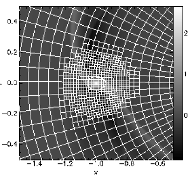
Figure 8: Close-up on the logarithm of the surface density near the planet. Overplotted is the AMR mesh structure, where each block consists of 8x8 cells.

Figure 9: Accretion rates onto a 1 $\mathrm{{M}_{J}}$ planet for three different methods of source term integration.

Figure 10: Accretion rates onto a 1 $\mathrm{{M}_{J}}$ planet for three different flux limiters.

7.1 High mass planet

We start by discussing the results for a $1$ $\mathrm{{M}_{J}}$ planet. Because this planet is able to open up a gap in the disk, the accretion rate is determined by the amount of mass that flows through the gap (Kley 1999), and less by the density structure close to the planet.

In Fig. 7 we show the accreted mass and the accretion rate as a function of time for our standard resolution, accretion parameters, source term integration and flux limiter (solid lines). Because we do not start with an initial gap the accretion rate is very high at the beginning of the simulation, dropping about one order of magnitude in $200$ orbits to a value of $2\leavevmode\nobreak\ 10^{-4}$ (disk masses per orbit). We ran one model to $500$ orbits, and the final accretion rate turned out to be $1.5\leavevmode\nobreak\ 10^{-4}$. The fact that the accretion rate approaches a constant value after about 500 orbits and the actual value found agree within a factor 2 with D’Angelo et al. (2002) and Lubow et al. (1999). The planet accretes approximately 10 percent of the total disk mass during the simulation.

7.1.1 Accretion parameters

The accretion procedure is described by two parameters: the radius within which we take out material ($r_{\mathrm{acc}}$) and the value of $f$ (see Eq. 49). We can vary these to see if this influences the final accretion rate.

In Fig. 7 the accretion rates onto a 1 $\mathrm{{M}_{J}}$ planet are shown for the standard case ($r_{\mathrm{acc}}=0.5$ $\rm{R_{R}}$ and $f=0.5$) and for parameters $r_{\mathrm{acc}}=0.1$ $\rm{R_{R}}$ and $f=5/3$ (the curve labeled with ’higher f’). The standard set was used by Kley (1999), and the other case by D’Angelo et al. (2002). Note that the accretion areas differ by a factor $25$, while $f$ varies only by a factor $3.3$. So for identical density distributions close to the planet the standard parameters yield $7.5$ times more accreted mass during one time step. Despite this the final accretion rate is the same for both sets of parameters.

Because of the different accretion radii any difference in accretion rate would imply that the flow within the Roche lobe is important for the accretion proces. Disk material that makes it to $0.5$ $\rm{R_{R}}$ is accreted for the standard parameters, while it has to make it all the way to $0.1$ $\rm{R_{R}}$ to be accreted in the second case. The fact that we do not see any differences indicates that the accretion rate is determined by the amount of mass the disk is able to supply, independent of local processes near the planet.

Figure 11: Accretion onto a 1/64 $\mathrm{{M}_{J}}$ planet. Left panel: total accreted mass in units of the initial disk mass. Right panel: accretion rate, in units of disk masses per orbit.

7.1.2 Resolution

Our base resolution corresponds to approximately 8 cells per $\rm{R_{R}}$, which means that the standard accretion area is resolved by only a few grid cells. This might be of influence on the inferred accretion rate, and therefore we performed simulations on different resolutions.

First of all we lowered the resolution with a factor of 2, the same resolution as in Kley (1999). In this case we do not resolve the Roche lobe, so if the flow close to the planet is important for accretion we would expect differences. However, since the two sets of accretion parameters did not yield different accretion rates we expect no big resolution effects. Indeed, Fig. 7 shows that for this low resolution case (dotted line) the accretion rate is the same as for our standard resolution. This shows that resolving the flow within the Roche lobe is not important for gap-opening planets, at least not for determining accretion rates.

It is computationally very expensive to go up a factor of 2 in resolution on the whole grid, therefore we used our AMR module to refine the region around the planet. Figure 8 shows a close-up on the density pattern after 20 orbital periods. Overplotted are the Roche lobe and the grid structure. Each block represents 8x8 cells, so that we have approximately 1500 cells within the Roche lobe. Therefore we can really resolve the flow inside the Roche lobe with this resolution. Nevertheless also this resolution yielded the same accretion rate of $2\leavevmode\nobreak\ 10^{-4}$ $\rm{M_{d}}P^{-1}$.

7.1.3 Equation of state

It is interesting to compare accretion rates for a truely isothermal simulation and a run that does include an energy equation, but at a very low adiabatic exponent $\Gamma$. This has been done before to mimic isothermal flow for planet-disk interaction (Nelson & Benz 2003). The basic idea is that for a low value of $\Gamma$ the gas can be compressed without a large change in temperature. In order to check the validity of this approach regarding planet-disk interaction, we ran simulations including an energy equation but with a low value of $\Gamma$.

We performed two simulations including an energy equation, one with $\Gamma=1.001$ and one with $\Gamma=1.01$. The latter value was also used by Nelson & Benz (2003). We found that the basic flow structures remain the same, and that the temperature profile does not change anywhere but very close to the planet. For $\Gamma=1.001$ the temperature rises already by a factor 10, and for $\Gamma=1.01$ by a factor of $60$. This steep temperature gradient slows down the gas flow towards the planet considerably.

Due to the higher temperatures close to the planet the accretion slows down. Already for $\Gamma=1.001$ the accretion rate drops by a factor of $2$, and even a factor of $10$ for $\Gamma=1.01$. This shows that the accretion rate depends very much on the temperature near the planet, and that ’nearly’ isothermal simulations can produce very different results from truely isothermal runs.

This effect is different from the one described in Kley (1999), who found that a polytropic equation of state leads to a reduction in the accretion rate. Because the temperature is proportional to the density in that case (for $\Gamma=2$), the gap region is much cooler and therefore the viscosity is reduced when the $\alpha$-formalism is used. In our case, there is a temperature rise very close to the planet, which leads to a pressure barrier that is able to slow down accretion considerably, even when $\Gamma$ is as low as $1.001$. Therefore we conclude that these kinds of simulations are not able to mimic isothermal flow for this specific case, due to the deep potential well of the planet.

7.1.4 Source term integration

In Fig. 3 we demonstrated that the way source terms are included has dramatic effects on the proces of gap formation. In this section we show that this also affects the accretion onto the planet.

Figure 9 shows the accretion rates for three different methods of source term integration: exact, hybrid and approximate extrapolation. See Sec. 6 for their definition. Again, as in Fig. 3 approximate extrapolation is the odd one out, yielding a 4 times lower accretion rate. This clearly has to do with the difference in gap formation time scale, and again it is clear that approximate extrapolation is not the way to go.

Both the exact and hybrid method give the same results. This is not surprising, because the region where the methods differ most is where the source terms are large: close to the planet. And as we mentioned before, this region is not important for the accretion rate.

Figure 12: Accretion onto a 1/8 $\mathrm{{M}_{J}}$ planet. Left panel: total accreted mass in units of the initial disk mass. Right panel: accretion rate, in units of disk masses per orbit.

7.1.5 Flux Limiter

The flux limiter did not play a major role in gap formation (see Fig. 5), only at the inner parts of the disk some differences can be seen. Figure 10 shows the accretion rates for the three different limiters discussed in Sec. 6. It is clear that the accretion rate does not depend at all on the flux limiter.

This can be understood if one realizes that it is the flow from the outer disk to the inner disk that governs the accretion rate (see Kley (1999)). But in the outer disk the waves are weaker than in the inner disk, so a different flux limiter should not change the mass flux from the outer disk very much.

7.2 Low mass planet

We now move to the other side of the planetary mass spectrum to investigate accretion onto planets that do not open gaps in the disk. Specifically we focus on a planet with mass $\rm{M_{J}}/64$. Because $\rm{R_{R}}\propto M_{\rm{p}}^{1/3}$ the Roche lobe of this planet is $4$ times as small as the Roche lobe of a jupiter-mass planet.

In Fig. 11 the solid line gives the accretion rate for our standard parameters and 4 levels of AMR. For our base resolution the Roche lobe would only be resolved by only 1 grid cell, clearly not enough to study accretion. Figure 11, dashed line, shows that 2 levels of refinement, yielding 4 cells per $\rm{R_{R}}$, is still not enough to reproduce the result for 4 levels of AMR. The accretion rates for 3 and 4 levels of AMR agree very well, showing that at least 8 cells per $\rm{R_{R}}$ are needed for accurately modeling accretion.

All accretion rates have reached their final value after $30$ orbits. The model with 4 levels of refinement was run until 200 orbits with no change in the accretion rate. This is because the planet does not open up a gap, which would take about $200$ orbits (see Sec. 6). The value of $3.5\leavevmode\nobreak\ 10^{-5}$ that we find is in good agreement with the results of D’Angelo et al. (2002). Note however that they need 7 grid levels, corresponding to approximately 6 levels of AMR for our simulations, while we need only 3 levels to obtain the same result.

Because we have already discarded the approximate extrapolation scheme in Sec. 6 and Sec. 6.1 we looked only at the difference between exact extrapolation and hybrid extrapolation for the low-mass case. However, we point out that in this case approximate extrapolation gave identical results. This is because the waves from this planet are too weak to make a difference in angular momentum flow. From Fig. 11 we see that both methods we considered for source term integration give identical results. In this case the planetary gravitational source terms are too small to cause a large difference in accretion rate.

Also different flux limiters gave identical results. In Fig. 11 we only show the superbee-result, but the minmod limiter yielded exactly the same accretion rate. This was to be expected, because in the limit of smooth flow (or, equivalently, no strong waves, as is the case for a low-mass planet) all limiters produce the same flux (see Eq. 31 with $a_{0}=a_{u}$).

Figure 13: Accretion rates onto a 1/8 $\mathrm{{M}_{J}}$ planet for the standard case (solid line), hybrid extrapolation (dotted line) and the minmod limiter (dashed line).

Figure 14: Left panel: accretion as a function of planet mass. Right panel: growth time (see Eq. 55). Filled circles indicate our standard result, diamonds give the results for the diffusive minmod limiter wherever they were different. In both panels the fit of D’Angelo et al. (2002) is shown by the dashed line.

7.3 Intermediate mass planet

The masses that lie in between the two extremes we have considered so far are perhaps the most interesting. In this regime the transition from linear disk response to gap formation takes place, and therefore also the transition from Type I to Type II migration. D’Angelo et al. (2002) find the highest accretion and migration rates here. Also, the cores of giant planets may well be in this mass range.

For this section we focus on a planet of mass $1/8$ $\mathrm{{M}_{J}}$, which makes its Roche lobe twice as small as for a Jupiter-sized planet. In Fig. 12 we compare the accretion rates for different resolutions. First of all, note that we need a relatively high resolution to obtain convergence (3 levels of refinement, which amounts to 16 cells per $\rm{R_{R}}$). This is already an indication that interesting things are going on. Secondly, we find an accretion rate that is about twice as low as was found by D’Angelo et al. (2002). In view of the good agreement for the low-mass planet this is remarkable.

In Fig. 13 we compare the standard model with the method of hybrid extrapolation and the minmod flux limiter. While for the high-mass planet as well as the low-mass planet these three methods gave identical results, for a $1/8$ $\mathrm{{M}_{J}}$ planet they differ significantly, giving a $66\leavevmode\nobreak\ \%$ and $100\leavevmode\nobreak\ \%$ higher accretion rate for the hybrid extrapolation and minmod limiter, respectively. With the most diffusive flux limiter we can reproduce the result of D’Angelo et al. (2002). This shows that numerical diffusion is a very important issue in these kinds of simulations.

It is not surprising that the diffusive minmod limiter increases the accretion rate, because it tends to smear out the strong density and velocity gradients near the planet, allowing mass to diffuse into the Roche lobe. For this planet local conditions determine the accretion rate, unlike the previous cases. Low-mass planets do not excite strong enough waves to alter their environment significantly, while high-mass planets open up gaps, and the accretion rate is therefore determined by the global evolution of the disk. Planets of intermediate mass, however, do not clear a gap while they excite reasonably strong waves, making the dynamics very interesting.

A similar story applies to the source term integration. We have seen no differences between exact and hybrid extrapolation for high and low-mass planets, while for our $1/8$ $\mathrm{{M}_{J}}$ planet the difference is quite dramatic. Again, the gravitational forces due to low-mass planets are too weak to cause a difference, while for high-mass planets the local conditions are irrelevant.

7.4 Dependence on planetary mass

In the previous sections we have looked in detail at three characteristic planetary masses. Here we focus on how the accretion rate depends on the mass of the planet. We have run simulations for planets from $0.5$ $\rm{M_{\oplus}}$ up to $8$ $\mathrm{{M}_{J}}$, or, in other words, from deep in the linear regime to well above the gap-opening mass.

In the left panel of Fig. 14 we show the accretion rate for all planetary masses, as well as the relation found by D’Angelo et al. (2002). As was mentioned in Sec. 7.2 the results for the low-mass planets agree very well with those found by D’Angelo et al. (2002). However, as soon as the disk response to the planet approaches the non-linear regime around $M_{p}\approx 0.1$ $\mathrm{{M}_{J}}$ the results start to differ significantly. At first, the accretion rate stays low, but around $M_{p}\approx 0.2$ $\mathrm{{M}_{J}}$ there is a strong rise leading to a maximum at $0.5$ $\mathrm{{M}_{J}}$, followed by a steep decline.

The general features of the plot are consistent with the results of D’Angelo et al. (2002): the accretion rate rises with planetary mass, with a maximum around $0.5$ $\mathrm{{M}_{J}}$, followed by a steeper decline. However, the rise as well as the decline are much more dramatic in our case, leading to a higher maximum accretion rate and lower accretion rates for the highest mass planets.

The diamonds in Fig. 14 represent the results obtained with the diffusive minmod limiter wherever they differed significantly from the standard case. We conclude that a diffusive flux limiter always tends to increase accretion onto the planet, especially in the mass regime in which the transition from linear to non-linear disk response takes place.

The difference between the results obtained with the minmod flux limiter and our standard limiter can be as large as $50\%$ (see Fig. 14). Because these differences are caused by purely numerical effects, one can interpret these as an estimate of the error in the values of the accretion rates in this mass regime. Keeping these error estimates in mind, we see that our results are roughly in agreement with the relation found by D’Angelo et al. (2002). Note, however, that our standard results always represent the lowest possible accretion rate. Different flux limiters or different source term integrations always lead to a higher accretion rate.

The growth time scale is defined as the time it takes for a planet to double its mass at a given accretion rate:

$$\tau_{\rm g}\equiv\frac{M_{\rm{p}}}{dM_{\rm{p}}/dt}$$ (55)

In order to express $\tau_{\rm g}$ in years we took a disk mass of $0.0035$ $\mathrm{{M}_{\odot}}$. When for a given mass $\tau_{\rm g}$ becomes comparable to the total disk life time the planet can not grow beyond this mass. This limiting mass is of the order of several $\mathrm{{M}_{J}}$ (D’Angelo et al. 2002). However, they do not consider planets more massive than $1$ $\mathrm{{M}_{J}}$.

In the right panel of Fig. 14 we show $\tau_{\rm g}$ for all planet masses. Again, the dashed curve shows the fit from D’Angelo et al. (2002). Because of the logarithmic scale on the y-axis the differences are much less pronounced. However, we still see the two different regimes and the sharp transition. Very important is the steep rise in $\tau_{\rm g}$ for the highest masses. Assuming that the planet spends maximal $10^{6}$ years inside this disk the maximum mass it can reach is $4$ $\mathrm{{M}_{J}}$. Note that if we exclude the planets more massive than $1$ $\mathrm{{M}_{J}}$ the slope of the growth time scale is in excellent agreement with the relation found by D’Angelo et al. (2002). Extrapolating this slope we would find that the maximum mass that can be reached is about $10$ $\mathrm{{M}_{J}}$. This shows that it is really necessary to include the highest mass planets to obtain a reliable estimate of the maximum planetary mass that can be reached through disk accretion.

The decline in accretion rate that we find for high-mass planets is steeper than found by Lubow et al. (1999), who used the ZEUS code for their simulations. We have shown that this is not due to the flux limiter or the source term integration, and the reason for this difference may be found in the intrinsic difference between the finite-difference approach and Riemann solvers. However, this is impossible to verify within our numerical method.

Figure 15: Torque exerted on a $1/8$ $\mathrm{{M}_{J}}$ planet, for three different flux limiters. The whole Roche lobe is excluded for these calculations.

Figure 16: Torque exerted on a $1/8$ $\mathrm{{M}_{J}}$ planet, for three different flux limiters. Only the inner half of the Roche lobe is excluded for these calculations.

8 Migration

It has become clear in recent years that protoplanets can be extremely mobile within their protoplanetary disk. Three types of migration can be distinguished: Type I, which concerns low-mass planets that do not open gaps in the disk , Type II for migration inside a clear gap, and Type III, for which the radial movement of the planet drives its migration (Masset & Papaloizou 2003). Because our planet stays at a fixed location, we are only dealing with Type I and Type II migration.

For the torque calculations, we exclude material orbiting within the Roche lobe of the planet, and we assume an initial disk mass of $0.0035$ $\mathrm{{M}_{\odot}}$.

8.1 Numerical Parameters

Migration rates turn out to be very robust once the Roche lobe as well as the disk scale height is well resolved. Across the whole mass spectrum we found no significant torque differences for the various methods of source term integration and flux limiters. Even approximate extrapolation, which was shown to lead to spurious numerical evolution of the gap, does not affect the torque on the planet. This is because for low-mass planets approximate extrapolation does not alter the density structure around the planet (see Sec. 7.2), and for high-mass planets it only speeds up gap formation, which leads to Type II migration.

As an example we show in Fig. 15 the torque as a function of time for a $1/8$ $\mathrm{{M}_{J}}$ planet for different flux limeters. All three limiters lead to a torque that is comparable to Type I migration. As with gap formation, the difference between $p=1.5$ and $p=1.0$ is larger than the difference between $p=1.5$ and $p=2.0$ (see Fig. 5), but for the torque the effect is not significant. This shows that the sensitivity of the accretion rate on numerical parameters found in Sec. 7.3 is due to effects inside the Roche Lobe, while we explicitly excluded this region for the torque calculations of Fig. 15.

This is further illustrated in Fig. 16, where we again show the total torque on the planet, but now we exclude only the inner half of the Roche lobe. The first thing to note is that the minmod limiter now gives a significantly different result compared to the other two. We found similar behaviour for the accretion rate in Sec. 7.3.

Secondly, we observe that the torque is less negative for $p=1.5$ and $p=1.0$. This is the torque reversal also observed by D’Angelo et al. (2002): material within the Roche lobe exerts a positive torque on the planet, slowing down migration. However, it is not clear exactly where the disk ends and the envelope of the planet starts. A gas giant is usually assumed to fill its Roche lobe during formation (Pollack et al. 1996), so all material orbiting inside the Roche lobe is part of the envelope. Therefore the question rises whether a planet should change its orbit due to its own envelope. On the other hand, important physical processes are not included in the current hydrodynamical simulations of planet-disk interaction, namely heat transport (due to the isothermal assumption) and self-gravity. Both can have dramatic influence on the direct surroundings of the planet, where the density is highest and the temperature may differ significantly from the ambient disk, and therefore it is not feasible yet to make a connection between the one-dimensional planet formation models of Pollack et al. (1996) and the hydrodynamic models of planet-disk interaction. For now, we are only interested in comparing our values to previous analytical and numerical results, which will be done in the next section.

Figure 17: Migration time scales for planets of different mass. Dashed line: analytical solution by Tanaka et al. (2002) for Type I migration. Dash-dotted line: result by Ward (1997) for Type II migration.

8.2 Dependence on planetary mass

For the low-mass case of Type I migration there exists a nice analytical prediction of the migration rate as a function of planetary mass (Tanaka et al. 2002). For gap-opening planets, the migration rate should not depend on planetary mass, only on the viscosity in the disk (Ward 1997). Numerical simulations show that in between these two extremes the fastest migration takes place, in two-dimensional simulations (D’Angelo et al. 2002) as well as in three-dimensional simulations (Bate et al. (2003); D’Angelo et al. (2003)).

In Fig. 17 we show the migration time scale $\tau_{\rm m}$ defined by:

$$\tau_{\rm m}=\frac{r_{\rm p}}{\left|v_{\rm r,p}\right|}$$ (56)

where the radial velocity of the planet due to a torque $\mathcal{T}$ is given by:

$$v_{\rm r,p}=2r_{\rm p}\frac{\mathcal{T}}{L_{\rm p}}$$ (57)

Here $\mathcal{T}$ is the torque due to the disk on the planet.

From Fig. 17 we see that we can reproduce Type I as well as Type II migration. The transition region extends approximately from $M_{\rm p}=0.1$ $\mathrm{{M}_{J}}$ to $M_{\rm p}=1.0$ $\mathrm{{M}_{J}}$, consistent with the three-dimensional results of Bate et al. (2003). A planet of mass $0.1$ $\mathrm{{M}_{J}}$ has the fastest migration time scale of approximately $10^{4}$ years.

Comparing Figs. 14 and 17 we see that for the low-mass planets the growth time scale is much shorter than the migration time scale, while for the high-mass planets it is the other way around. In the intermediate case, both time scales are approximately equal.

9 Summary and conclusion

We have presented a new method for modeling disk-planet interaction. Key features of the RODEO method are: it is a conservative method, it treats shocks and discontinuities correctly, and it uses stationary extrapolation to integrate the geometrical and gravitational source terms.

We found that the RODEO method performs very well on the problem of disk-planet interaction, not in the least because we do not experience serious computational difficulties as for example in Kley (1998). We have shed some new light on this matter in that this instability can be seen to result from the failure of most hydrodynamic schemes to recognize stationary states.

We find that the proces of gap formation crucially depends on source term integration. Only exact and hybrid extrapolation produce gaps of correct width. A diffusive flux limiter leads to a more pronounced inner edge of the gap.

The accretion rates turn out to be very robust in the low-mass regime ($M_{\rm p}<0.1$ $\mathrm{{M}_{J}}$) as well as in the high-mass regime ($M_{\rm p}>=1.0$ $\mathrm{{M}_{J}}$): they are independent of numerical resolution, accretion parameters and source term integration. A different equation of state affects the accretion rates significantly: even a very low $\Gamma$ of $1.001$ that is used frequently to mimic isothermal flow the accretion rate drops by a factor of $2$.

For intermediate mass planets the accretion rates are far less certain. They are dependent on the flux limiter used as well as on the way source terms are integrated. Within our method we find differences of $50\%$, and the differences between our results and the similar study of D’Angelo et al. (2002) are of the same order. This shows that the error bars on these values are very large.

For the highest mass planets we find significantly lower accretion rates than in previous numerical studies, limiting the maximum planet mass that can be reached to about 4 $\mathrm{{M}_{J}}$. Note that this is in fact the first numerical study that consistently goes beyond this limiting mass so that no extrapolation is required.

Migration rates are far more robust than accretion rates, as long as we limit the disk region that exerts a torque on the planet to outside the planetary Roche lobe. Therefore the region where most differences arise in the accretion rates is located deep within the Roche lobe.

We can nicely reproduce the analytical results for Type I and Type II migration, with a transition region extending from $M_{\rm p}=0.1$ $\mathrm{{M}_{J}}$ to $M_{\rm p}=1.0$ $\mathrm{{M}_{J}}$. In this transition region the fastest migration rate corresponds to a mass of $0.1$ $\mathrm{{M}_{J}}$.

The RODEO method can also be used for two-fluid calculations (see Paardekooper & Mellema (2004)) to model dust-gas interaction in protoplanetary disks. Also, the method can easily be extended to three dimensions, and is also suited to treat an energy equation in a multi-dimensional set-up. We will consider these extensions in forthcoming papers.

Appendix A Explicit expressions

Here we give explicit expressions of the eigenvalues, eigenvectors and projection coefficients for the isothermal Euler equations in cylindrical coordinates.

A.1 Radial direction

The Jacobian matrix $\mathcal{A}$ is given by:

$$\mathcal{A}=\left(\begin{array}[]{ccc}0&1&0\\ c_{s}^{2}-v_{r}^{2}&2v_{r}&0\\ -v_{r}v_{\phi}&v_{\phi}&v_{r}\end{array}\right)$$ (58)

The eigenvalues of this matrix are:

$$\lambda_{1} = v_{r}-c_{s}$$

$$\lambda_{2} = v_{r}+c_{s}$$ (59)

$$\lambda_{3} = v_{r}\leavevmode\nobreak\ \leavevmode\nobreak\ \leavevmode\nobreak\ \leavevmode\nobreak\ \leavevmode\nobreak\ \leavevmode\nobreak\$$

The corresponding eigenvectors:

$$\@vec{e}_{1} = \left(1,v_{r}-c_{s},v_{\phi}\right)$$

$$\@vec{e}_{2} = \left(1,v_{r}+c_{s},v_{\phi}\right)$$ (60)

$$\@vec{e}_{3} = \left(0,0,1\right)\leavevmode\nobreak\ \leavevmode\nobreak\ \leavevmode\nobreak\ \leavevmode\nobreak\ \leavevmode\nobreak\ \leavevmode\nobreak\ \leavevmode\nobreak\ \leavevmode\nobreak\ \leavevmode\nobreak\$$

A vector $\@vec{\Delta}\equiv(\Delta_{\rho},\Delta_{r},\Delta_{\phi})$ can be projected on these eigenvalues using the following projection coefficients, found by solving the system $\mathcal{C}\@vec{a}=\@vec{\Delta}$, where $\mathcal{C}$ is the matrix with the eigenvectors:

$$a_{1} = \frac{1}{2c_{s}}((c_{s}+v_{r})\Delta_{\rho}-\Delta_{r})$$

$$a_{2} = \frac{1}{2c_{s}}((c_{s}-v_{r})\Delta_{\rho}+\Delta_{r})$$ (61)

$$a_{3} = \Delta_{\phi}-v_{\phi}\Delta_{\rho}\leavevmode\nobreak\ \leavevmode\nobreak\ \leavevmode\nobreak\ \leavevmode\nobreak\ \leavevmode\nobreak\ \leavevmode\nobreak\ \leavevmode\nobreak\ \leavevmode\nobreak\ \leavevmode\nobreak\ \leavevmode\nobreak\ \leavevmode\nobreak\ \leavevmode\nobreak\ \leavevmode\nobreak\ \leavevmode\nobreak\ \leavevmode\nobreak\$$

A.2 Azimuthal direction

The Jacobian matrix $\mathcal{A}$ is given by:

$$\mathcal{A}=\left(\begin{array}[]{ccc}0&1&0\\ -v_{r}v_{\phi}&v_{\phi}&v_{r}\\ \frac{c_{s}^{2}}{r^{2}}-v_{\phi}^{2}&0&2v_{\phi}\end{array}\right)$$ (62)

The eigenvalues of this matrix are:

$$\lambda_{1} = v_{\phi}-c_{s}/r$$

$$\lambda_{2} = v_{\phi}+c_{s}/r$$ (63)

$$\lambda_{3} = v_{\phi}\leavevmode\nobreak\ \leavevmode\nobreak\ \leavevmode\nobreak\ \leavevmode\nobreak\ \leavevmode\nobreak\ \leavevmode\nobreak\ \leavevmode\nobreak\ \leavevmode\nobreak\ \leavevmode\nobreak\$$

The corresponding eigenvectors:

$$\@vec{e}_{1} = \left(1,v_{r},v_{\phi}-c_{s}/r\right)$$

$$\@vec{e}_{2} = \left(1,v_{r},v_{\phi}+c_{s}/r\right)$$ (64)

$$\@vec{e}_{3} = \left(0,1,0\right)\leavevmode\nobreak\ \leavevmode\nobreak\ \leavevmode\nobreak\ \leavevmode\nobreak\ \leavevmode\nobreak\ \leavevmode\nobreak\ \leavevmode\nobreak\ \leavevmode\nobreak\ \leavevmode\nobreak\ \leavevmode\nobreak\ \leavevmode\nobreak\ \leavevmode\nobreak\$$

A vector $\@vec{\Delta}\equiv(\Delta_{\rho},\Delta_{r},\Delta_{\phi})$ can be projected on these eigenvalues using the following projection coefficients, found by solving the system $\mathcal{C}\@vec{a}=\@vec{\Delta}$, where $\mathcal{C}$ is the matrix with the eigenvectors:

$$a_{1} = \frac{1}{2c_{s}}((c_{s}+rv_{\phi})\Delta_{\rho}-r\Delta_{\phi})$$

$$a_{2} = \frac{1}{2c_{s}}((c_{s}-rv_{\phi})\Delta_{\rho}+r\Delta_{\phi})$$ (65)

$$a_{3} = \Delta_{r}-v_{r}\Delta_{\rho}\leavevmode\nobreak\ \leavevmode\nobreak\ \leavevmode\nobreak\ \leavevmode\nobreak\ \leavevmode\nobreak\ \leavevmode\nobreak\ \leavevmode\nobreak\ \leavevmode\nobreak\ \leavevmode\nobreak\ \leavevmode\nobreak\ \leavevmode\nobreak\ \leavevmode\nobreak\ \leavevmode\nobreak\ \leavevmode\nobreak\ \leavevmode\nobreak\ \leavevmode\nobreak\ \leavevmode\nobreak\ \leavevmode\nobreak\ \leavevmode\nobreak\$$

References

- Artymowicz (2004) Artymowicz, P. 2004, in ASP Conf. Ser. 324: Debris Disks and the Formation of Planets, 39–+
- Balbus & Hawley (1990) Balbus, S. A. & Hawley, J. F. 1990, BAAS, 22, 1209
- Bate et al. (2003) Bate, M. R., Lubow, S. H., Ogilvie, G. I., & Miller, K. A. 2003, MNRAS, 341, 213
- Beckwith & Sargent (1996) Beckwith, S. V. W. & Sargent, A. I. 1996, Nature, 383, 139
- Boss (1997) Boss, A. P. 1997, Science, 276, 1836
- Bryden et al. (1999) Bryden, G., Chen, X., Lin, D. N. C., Nelson, R. P., & Papaloizou, J. C. B. 1999, ApJ, 514, 344
- Cameron (1978) Cameron, A. G. W. 1978, Moon and Planets, 18, 5
- D’Angelo et al. (2002) D’Angelo, G., Henning, T., & Kley, W. 2002, A&A, 385, 647
- D’Angelo et al. (2003) D’Angelo, G., Kley, W., & Henning, T. 2003, ApJ, 586, 540
- De Val-Borro et al. (2005) De Val-Borro, M., Edgar, R., Gawryszczak, A., et al. 2005, MNRAS, in preparation
- Eulderink & Mellema (1995) Eulderink, F. & Mellema, G. 1995, A&AS, 110, 587
- Gammie (1996) Gammie, C. F. 1996, ApJ, 457, 355
- Godon (1996) Godon, P. 1996, MNRAS, 282, 1107
- Goldreich & Tremaine (1980) Goldreich, P. & Tremaine, S. 1980, ApJ, 241, 425
- Kley (1998) Kley, W. 1998, A&A, 338, L37
- Kley (1999) Kley, W. 1999, MNRAS, 303, 696
- Kley (2000) Kley, W. 2000, MNRAS, 313, L47
- Lin & Papaloizou (1986) Lin, D. N. C. & Papaloizou, J. 1986, ApJ, 309, 846
- Lin & Papaloizou (1993) Lin, D. N. C. & Papaloizou, J. C. B. 1993, in Protostars and Planets III, 749–835
- Lubow et al. (1999) Lubow, S. H., Seibert, M., & Artymowicz, P. 1999, ApJ, 526, 1001
- MacNeice et al. (2000) MacNeice, P., Olson, K. M., Mobarry, C., de Fainchtein, R., & Packer, C. 2000, Computer Physics Communications, 126, 330
- Masset & Papaloizou (2003) Masset, F. S. & Papaloizou, J. C. B. 2003, ApJ, 588, 494
- Mellema et al. (1991) Mellema, G., Eulderink, F., & Icke, V. 1991, A&A, 252, 718
- Nelson & Benz (2003) Nelson, A. F. & Benz, W. 2003, ApJ, 589, 556
- Nelson & Papaloizou (2003) Nelson, R. P. & Papaloizou, J. C. B. 2003, MNRAS, 339, 993
- Nelson et al. (2000) Nelson, R. P., Papaloizou, J. C. B., Masset, F., & Kley, W. 2000, MNRAS, 318, 18
- Paardekooper & Mellema (2004) Paardekooper, S.-J. & Mellema, G. 2004, A&A, 425, L9
- Pollack et al. (1996) Pollack, J. B., Hubickyj, O., Bodenheimer, P., et al. 1996, Icarus, 124, 62
- Pringle (1981) Pringle, J. E. 1981, ARA&A, 19, 137
- Rafikov (2002) Rafikov, R. R. 2002, ApJ, 572, 566
- Rafikov (2005) Rafikov, R. R. 2005, ApJ, 621, L69
- Roe (1981) Roe, P. L. 1981, J. Comp. Phys, 43, 357
- Shakura & Sunyaev (1973) Shakura, N. I. & Sunyaev, R. A. 1973, A&A, 24, 337
- Sod (1978) Sod, G. A. 1978, J. Comp. Phys, 27, 1
- Strang (1968) Strang, G. 1968, Siam. J. Num. Analysis, 5, 506
- Tanaka et al. (2002) Tanaka, H., Takeuchi, T., & Ward, W. R. 2002, ApJ, 565, 1257
- van Leer (1977) van Leer, B. 1977, Journal of Computational Physics, 23, 276
- Ward (1997) Ward, W. R. 1997, Icarus, 126, 261
- Woodward & Colella (1984) Woodward, P. & Colella, P. 1984, J. Comp. Phys, 54, 115