Circular Polarimetry and the Line of Sight to the BN Object

Abstract

The 3.1 $\mu$m absorption feature of water-ice has been observed spectroscopically in many molecular clouds and, when it has been observed spectropolarimetrically, usually a corresponding polarization feature is seen. Typically on these occasions, and particularly for the BN object, a distinct position angle shift between the feature and continuum is seen, which indicates both a fractionation of the icy material and a changing alignment direction along the line of sight.

Here the dependence of circular polarimetry on fractionation along the line of sight is investigated and it is shown that the form of its spectrum, together with the sign of the position angle shift, indicates where along the line of sight the icy material lies. More specifically a coincidence between the sign of the position angle displacement in the ice feature, measured north through east, and that of the circular polarization ice feature means that the icy grains are overlaid by bare grains. Some preliminary circular polarimetry of BN has this characteristic and a similar situation is found in the only two other cases for which relevant observations so far exist.

1 Introduction

In astronomy various materials may lie along the line of sight and their nature clarified by spectroscopy and spectropolarimetry; where these materials may lie can only be inferred. Circular polarimetry provides a means that can directly probe relative position along the line of sight.

Molecular vibrations in the solid state give rise to features in the near and mid-infrared which are characteristic of the chemistry of the material. Infrared spectroscopy has been used to probe the chemical nature of interstellar dust, the solid component of the interstellar medium (ISM). In this way it has been found that the dust exists as small submicron sized grains of which a ubiquitous component is a silicate-like material, but other constituents without an infrared signature such as carbon must be present, and the existence of various ices and refractory materials depend on the local environment: for example ice features are only observed within dense clouds.

Because the grains are in general non-spherical and are often aligned and oriented by the ambient magnetic field the extinction will differ for E vectors parallel and orthogonal to this projected direction (dichroism) and the the radiation traversing the medium becomes polarised. A phase change between these orthogonal directions is also introduced (birefringence) and circular polarization will be produced if the alignment direction changes along the line of sight (Serkowski 1962). Apart from very small effects the position angle remains independent of wavelength except if the dust composition also changes along the line of sight, in which case the position angle of the different molecular species will be different. Thus a changing position angle at the characteristic wavelengths of different dust species indicates both fractionation and changing alignment direction. Such effects are often observed when linear polarization studies have been made of ice features towards sources in dense clouds (eg Hough etal 1989, 1996; Holloway etal 2002), and only polarimetry can demonstrate this line of sight structure so directly. In the near infrared circular polarization has been obseved in the direction of the Becklin Neugebauer (BN) object in Orion by Serkowski and Rieke (1973), and from several molecular cloud sources by Lonsdale etal (1980) and Dyck and Lonsdale (1980) and a twist of alignment direction must exist to yield the observed circular polarization. Hough etal (1996) observed a position angle change of several degrees in the linear polarization of the ice feature in BN and this additionally requires that the icy material is fractionated along the line of sight. Neither the intensity spectrum nor the polarization spectrum are sensitive to the details of the fractionation other than the existence of an alignment twist and the sign of the angular displacement between the components. Conversely circular polarization does depend on the sign of twist and on the ordering of materials along the line of sight; in this sense it is not commutative, and the purpose of this paper is to show how this can be turned to practical use.

2 Circular polarization from changing grain alignment

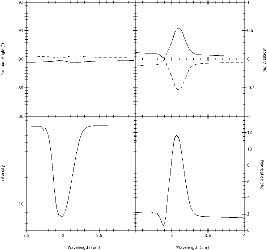
Figure 1: Intensity, linear polarization, position angle and circular polarization produced by two identical regions of H₂O mantles on silicate grains with grain alignments at 100^∘ and 80^∘. Solid lines denote the 100^∘ region preceeding the 80^∘ region and dotted lines the inverse. Extinction (hence the intensity) and linear polarization are unaffected by reversal while circular polarization inverts and the position angle departs very slightly from the mean of the alignment angles as it is displaced towards the last alignment direction. The position angle is weakly wavelength dependent. The grains are of ‘astrosilicate’ cores with mantles of pure water-ice.

Figure 2: As for Fig 1 except that the icy mantles have been removed from the second region. The ice feature vanishes from circular polarization on reversal and the position angle spectrum is barely changed.

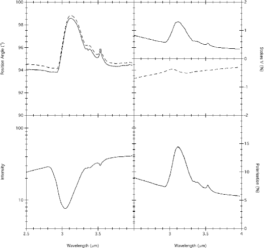
Figure 3: Observed circular and linear polarizations in the region of the ice feature for model AC13 in Table 1.

Circular polarization can arise in a number of ways but in the interstellar medium always as a secondary process: through (a) scattering of polarized light by dust grains, (b) scattering of unpolarized light by aligned non spherical grains, (c) by passage of linearly polarised light through a medium of aligned nonspherical grains. In the latter case the medium is birefringent through the presence of aligned grains and circular polarization is produced so long as the alignment direction is neither parallel nor orthogonal to the linear polarization. In the nearer infrared the former two processes are important and can yield high percentatages of circular polarization, but it is the latter process that is of interest here as the sign and spectral form of the circular polarization depend on the twist between the regions and their distribution along the line of sight.

Polarization produced by a medium with changing grain alignment is discussed by Martin (1974, 1978), who treats analytically the case of uniform slabs of differing polarization properties at varying angles to each other, and also that of a continuous medium with uniform twist. Much of what is presented here was inspired by and derives from Martin’s 1974 paper but the analysis concentrates more explicitly on what can be learned from the combination of linear and circular polarimetry. In the two slab case Martin (1974) points out that the circular polarization, $V/I$, depends on the linear dichroism of the first slab, the linear birefringence of the second slab, and the angle between the two slabs, so that it is sensitive to the sequence of material changes along the line of sight. In his treatment Martin neglects some minor terms to make the integration more tractable and, because the treatment is analytic, he derives useful and instructive relationships governing both the amount and sign of the circular polarization and the amount of position angle change in the linear polarization. In this study a numerical approach is adopted which is more convenient for the display of the wavelength dependence of specific models of ice mantled grains and can use the full polarization transfer.

Following Martin (1974) two slab and uniformly twisted models are considered. For the two slab case the two regions along the line of sight each contain a uniform grain population in respect of shape, chemistry and alignment. These properties can differ between the two regions as can their extinction. In the single twisted region the change in grain properties is introduced at a discrete twist angle. The initial radiation is unpolarized and independent of wavelength, a simplification that does not affect the polarization. Grains are taken as oblate with cross sections for absorption and phase determined from the real and imaginary parts of the electric polarizability in the Rayleigh limit (eg Draine and Lee 1984) and grain mantles are assumed confocal. The polarization cross sections for oblate grains, $C_{pol}=C_{abs}^{\perp}-C_{abs}^{\parallel}$, where $C_{abs}^{\perp}$ and $C_{abs}^{\parallel}$ are the absorption cross sections for E vectors perpendicular and parallel to the symmetry axes, determine the dichroism of the medium along the line of sight through $C_{pol}\,R\,$cos${}^{2}\delta$, where $\delta$ is the angle between alignment direction and the plane of the sky. Here $R=\frac{3}{2}(<$cos${}^{2}\beta>-\frac{1}{3})$ is the Rayleigh reduction factor for spinning grains precessing with angle $\beta$ about the alignment direction (Greenberg 1968). Thus $C_{pol}\,R\,$cos${}^{2}\delta$ is the effective cross section for polarized intensity in the plane of the sky. In a similar way $C_{crc}=C_{pha}^{\perp}-C_{pha}^{\parallel}$, where the $C_{pha}$’s are the respective cross sections for phase advance, determine the birefringence of the medium through $C_{crc}\,R\,$cos${}^{2}\delta$. The extinction cross section is

$$C_{abs}=\frac{2C_{abs}^{\perp}+C_{abs}^{\parallel}}{3}-\frac{RC_{pol}}{6}(3\rm{cos}^{2}\delta-2)$$

and the second term can usually be ignored. Expressions for $C_{abs}^{\perp}$, $C_{abs}^{\parallel}$, $C_{pha}^{\perp}$ and $C_{pha}^{\parallel}$ for oblate grains follow Draine and Lee (1984).

The polarization transfer equations (see Appendix) are iterated through each slab in turn and the two slabs are then reversed to determine effects due to ordering along the line of sight.

Martin (1974) gives a number of relations between the linear and circular polarization and the position angle which can be applied in the case of two slabs. Denoting by $\theta_{1}$ and $\theta_{2}$ the alignment direction in the first and second slabs and by $r$ the ratio $p_{2}/p_{1}$ of the linear polarizations produced in the second to first slabs then the depolarization is given by $D=\sqrt{(1+2r\,\textrm{cos}(2\phi)+r^{2})}/(1+r)$ (Martin 1974, equation 24), where $\phi=\theta_{2}-\theta_{1}$, and the position angle, $\theta$, of the resultant is given by (Martin 1974, equation 27) tan $2(\theta-\theta_{1})=r\,$sin$\,2\phi/(1+r\,$cos$\,2\phi)$. So long as the grains in the two slabs have the same chemistry (and shape), $r=p_{2}/p_{1}$ is independent of wavelength and so is the position angle, $\theta$. If the grains in one of the slabs displays extra polarization at some wavelength which changes $r$ to $r_{f}$ then there will be a position angle change

$$\textrm{tan}\,2\Delta\theta=(r_{f}-r_{c})\,\textrm{sin}\,2\phi/(1+r_{f}r_{c}+(r_{f}+r_{c})\textrm{cos}\,2\phi),$$

where $r_{c}$ is the polarization ratio at other wavelengths. If the slabs are interchanged the linear polarization and position angle are unchanged ($\phi$ changes sign, $r_{f}$ and $r_{c}$ invert) in this approximation. Only the circular polarizaton changes, both in sign and character.

Approximations in these relations compared to a full polarization transfer depend on the dielectic functions involved but are usually negligible so long as the polarizations are small. As an example in Fig 1 both slabs contain identical “astrosilicate” (Draine and Lee 1984, Draine 1985) cores with water-ice mantles (Hudgins etal 1993) at an angle of 20^∘. Continuous lines are for a 100^∘ aligned slab preceeding an 80^∘ slab and the broken line is the reversed situation. There is no position angle change in the ice feature but a very small change of $\sim 0.1^{\circ}$ displaced from the mean towards the second slab in each case. The circular polarization inverts and has a spectral form similar to the linear polarization whose change is undetectable in the figure.

As a further example we take the slabs to contain grains with an “astrosilicate” core with and without a water-ice mantle; Fig 2 shows that the linear polarization and the position angle are independent of the order of the slabs to a very close approximation, while the circular polarization displays the ice feature only when the icy slab precedes the other along the line of sight. After interchanging just a reversed sign continuum remains with little evidence for structure, and what structure remains is spectrally different from either the scaled down unreversed circular or linear polarization. The small changes seen in the position angle are due to the full polarization transfer; very small changes to the linear polarization are not discernable.

More generally, following Martin (1974), for dissimilar slabs the circular polarization is dominated by the spectral properties of the first slab, and its sign by the handedness of the alignment twist; positive sign indicates an alignment angle increasing (north through east) with increasing depth, or equivalently a clockwise twist in the direction towards the observer. If the position angle shift of a component has he same sign as the circular polarization that component must be further down the line of sight (than what produces the continuum) and vice versa.

3 A model of the line of sight to BN

In Fig 2 the pure H₂O ice feature is narrower than the observed feature and the background continuum level is not well reproduced by “astrosilicate” alone. The extinction declines rapidly from its peak to $3.3\mu$m and then shows a slower decrease in an extended wing to 3.6$\mu$m and this is reproduced in the linear polarization with the wing being slightly more prominent. Such structure, different from pure H₂O ice, has been observed in the spectrum of many young stellar objects (Smith, Sellgren and Tokunaga 1989) and attributed to the presence of other ices such as NH₃ and/or CH₃OH. There is considerable variation in the extinction profile of the young stellar objects observed by Smith, Sellgren and Tokunaga and BN appears to be an extreme case with a pronounced narrow additional absorption feature at 3.08$\mu$m, which was interpreted as requiring a range of temperatures of H₂O ices up to 150K.

Modelling of the material along the line of sight to BN which includes polarimetric observations has been done by Lee and Draine (1985). As a starting point they used the MRN graphite-silicate model (Mathis, Rumpl, and Nordsieck 1977) using bare oblate grains of ‘astronomical silicate’ and graphite, and these grain cores mantled with an H₂O:NH₃ mixture and obtained a satisfactory match to the then existing linear polarimetry around the ice feature and in the mid infrared (Capps, Gillett and Knacke 1978, Capps 1976). To reproduce the circular polarization observations of Lonsdale et al (1980) at 2.2$\mu$m and Serkowski and Rieke (1973) at 3.45$\mu$m they used a twist angle of $\phi\simeq 25^{\circ}$ confined to the region containing the core/mantled grains, and this predicted circular polarization close to 1% which indicated the presence of an ice feature.

Hough etal (1996) presented high quality spectropolarimetry of the ice feature which revealed a distinct position angle shift between the feature and continuum. Because of this evidence of fractionation of the ice along the line of sight they used a two slab model in which bare and mantled grains were in separate regions with an angle of 10-25^∘ between them, to produce the observed 4^∘ position angle shift.

Modelling has also been presented by Holloway (2003) who produced greatly improved fits in the mid-infrared by using amorphous olivine (Dorschner etal 1995) in place of ‘astrosilicate’ and amorphous carbon (Zubko etal 1996) in preference to graphite. There are some small discrepancies between the polarization properties of BN reported by Hough etal (1996) and Holloway etal (2002) in the wavelength region around and short of 3.0$\mu$m. These differences concern the detailed shape of the polarization, and not the levels of feature and continuum polarization and do not affect the way the present modelling is performed. Nevertheless it is important that the spectropolarimetric observations of BN, and other objects, are repeated.

Following Hough etal 1996 we use the dielectric function of the “strong” ice mixture of Hudgins etal (1993), containing H₂O, CH₃OH, CO and NH₃ in the ratio 100:50:1:1, but here use the temperature of 120^∘K as mantles on silicate and carbon cores, together with bare grains of silicate and carbon. Bare grains are taken as oblate with the mantles confocal on identical cores, and cross-sections found in the Rayleigh limit using equations in Draine and Lee (1984). Draine’s (1985) “astrosilicate” dielectric function is used but the dielectric function for crystalline graphite depends on the direction of its c-axis with respect to the radiation E vector; $\epsilon_{\parallel}$ and $\epsilon_{\perp}$ represent E vectors parallel and perpendicular to this axis, and are very different functions of $\lambda$. An approximation is made (Draine and Lee 1984) that $1/3$ of the grains have the isotropic dielectric function $\epsilon_{\parallel}$ and $2/3$ have the isotropic dielectric function $\epsilon_{\perp}$. The corresponding cross sections are computed and their sum taken as representing a random distribution of graphite c-axes within the grain; bare and core graphite grains are both treated in this way. Partly because of the approximations made for graphite, cross sections based on an amorphous carbon dielectric function from Zubko etal (1996) are also used and referred to as ACAR.

Recently Robberto etal (2005) have placed the extinction to the BN object at $\tau_{9.8\mu}=1.37$ from a fit to filter photometry through the silicate feature. However they ignore the presence of underlying silicate emission (Gillett etal 1975; Aitken etal 1981) indicated by single aperture spectroscopy and the fit then indicates a much larger extinction of $\tau_{10\mu}=3.3$, which is the value for the $\tau_{10\mu}$ used here. An additional and independent factor confirming this larger value is the observed absorptive polarization of 12.5% at 10$\mu$m (Aitken, Smith, Roche, 1989), making its specific polarization $p/\tau$ = .125/3.3 = .038, the largest for galactic sources out of a sample of 30 (Smith etal 2000). The constraint on the amount of the “strong” ice mixture is provided by the depth of the ice extinction $\tau_{3.1\mu}=1.6$. The ratio of carbon/silicate has been taken as 0.7 by number, which is between the MRN value of .87 and that used by Lee and Draine, of .45 in their case A.

Further observational constraints are provided by the linear polarizations of 12.5% at 10$\mu$m, 16% at the peak of the ice feature at 3.1$\mu$m and its continuum of 8.5% at 3.6$\mu$m (Hough etal 1996). At this stage no contraints are derived from the circular polarization or the position angle of the linear polarization. To restrict the number of free parameters bare grains and grain cores of silicate and carbon are taken to be the same size and oblate and the ratio of mantled to bare grains is taken as the same for silicate as for graphite/carbon.

The above constraints and assumptions together with the cross sections of the grains for extinction define the column density of the bare and the mantled grains. The number ratio bare/mantled grains is then 2.7 if the volume ratio mantle/core, $v_{m}/v_{c}$=1, and 4.55 if $v_{m}/v_{c}$=1.5, implying a correspondingly larger column depth of bare grains than mantled. Linear polarizations and polarization cross-sections are then enough to determine three of the polarization reduction factors in terms of the fourth and this restricts the physically significant reduction factors to a continuum range shown sampled in Table 1, for $b/a=2.0$ ($a$ is the symmetry axis and $v_{m}/v_{c}$=1: $R_{sm}$ for ice mantles on silicates, $R_{gm}$ for ice on graphite/carbon, $R_{s}$ for bare silicates, and $R_{g}$ for bare carbon. Estimated in this way the the reduction factors contain the cos${}^{2}\delta$ term due to an alignment angle, $\delta$, out of the plane of the sky, and the effect of any fluctuations along the line of sight, so that the tabled reduction factors will represent lower limits. Grains with $v_{m}/v_{c}=1.0$ and $v_{m}/v_{c}=1.5$ for $b/a=1.5$ were also considered but are not presented here as they required seemingly implausibly large reduction factors to reproduce the observed linear polarizations.

This method does not attempt to fit properties such as feature width, shape or precise peak wavelength which may depend on many minor constituents and a range of physical conditions. The main intention here is to use the major ingredients and find a range of reduction factors which reproduce the observed levels of extinction and linear polarization in the feature and continuum and investigate how these are constrained by the observed position angle shift and what circular polarization is predicted by different sequences.

Table 1
Polarization reduction factors
for b/a=2.0 and $v_{m}/v_{c}$=1.0
label	reduction factors
	$R_{sm}$	$R_{gm}$	$R_{s}$	$R_{g}$
amorphous carbon (ACAR)
AC11	.129	.269	.083	0
AC12	.166	.214	.069	.025
AC13	.189	.180	.060	.04
AC14	.204	.158	.055	.05
AC15	.241	.102	.041	.075
AC16	.279	.047	.027	.1
AC17	.310	.001	.015	.121
graphite
GR11	0	.275	.119	.0385
GR12	.0194	.256	.112	.05
GR13	.065	.211	.093	.075
GR14	.111	.166	.075	.1
GR15	.156	.121	.057	.125
GR16	.202	.076	.039	.15
GR17	.248	.031	.021	.175
GR18	.278	0	.008	.192

The range of reduction factors is bounded when the contribution from one of them becomes zero or greater than unity, the extremes corresponding to no alignment and complete alignment lying in the plane of the sky. For ACAR, as $R_{g}$ increases from zero to a significant fraction, the dominant changes are for the mantled grains where $R_{gm}$ decreases from a substantial value to end the range without alignment while $R_{sm}$ increases to substantial alignment from smaller values, and the alignment efficiency of bare silicates reduces in compensation. When graphite replaces ACAR the behaviour of the reduction factors is broadly similar except that mantled silicates start the sequence with $R_{sm}=0$. Use of the MRN number ratio of carbon/silicate grains ($\simeq.9$) gave a very much truncated range of larger reduction factors than in the table. As was found before by Lee and Draine (1985) mantled grains need a greater alignment efficiency than bare to reproduce the observations, and they concluded that the magnetic field must be highly ordered and close to the plane of the sky, at least for the mantled grains. The lower polarization efficiency for bare grains suggests a poorer alignment mechanism of these grains compared with mantled grains but this idea was not favoured by Lee and Draine, partly on account of the lack of excess polarization in GL 2591 (Dyck and Lonsdale 1981) even though it shows strong ice absorption.

All of the sequences of polarization efficiencies in Table 1 yield the linear polarization properties of BN in the 2.4–4$\mu$m region to a good approximation except for depolarization due to twist of the alignment direction: here the depolarization factor $D\raisebox{-2.58334pt}{$\,\stackrel{{\scriptstyle\raisebox{-0.60275pt}{$\textstyle>$}}}{{\sim}}\,$}0.8$.

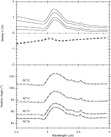
Figure 4: Circular polarization (top) and position angle (bottom) for a sample of the two-slab sequences from Tables 1 and 2. Sequences in each panels increase from the top curve to the bottom, as shown. Reversal is shown by the dashed lines. The lower continuum with increasing sequence number is because the linear polarization continuum produced in slab1 is decreasing at the expense of that produced in slab2.

3.1 Simple two component models

3.1.1 A simple two-slab model

To begin with a two slab model is considered in which only ice mantled grains are present in the first slab and only bare grains in the second.

For a particular sequence in Table 1 the only remaining free parameter is the angular twist, $\phi$, between the slabs, and this is varied until the position angle shift in the ice feature is $\Delta\theta=+4^{\circ}$, which is that observed for BN. This value of $\Delta\theta$ is not attainable with sequence AC11 because when $R_{g}$ is near zero very little linear polarization can be produced in the second slab by the “astrosilicate” alone, both $r_{f}$ and $r_{c}$ are small and even a twist $\phi=50^{\circ}$ only produces $\Delta\theta=1.5^{\circ}$ (cf equation 27, Martin 1974 and section 2). When $R_{g}$= 0.025 (AC12) a twist between the slabs of 41^∘ gives the observed $\Delta\theta=+4^{\circ}$ and as $R_{g}$ increases the required twist reduces further.

Table 2 gives the derived circular polarizations from this simple 2-slab model using the reduction factors from Table 1 and adjusting $\phi$ to give $\Delta\theta=+4^{\circ}$ when possible. Purely for computing and display convenience the two slab angles are equispaced about 90^∘ to give $\phi$, and $\theta_{p}$ is the position angle at the peak of the ice feature with reference to this frame. The observed position angle of this feature is 118^∘ for BN, and simple arithmetic enables the angles for slab1 to be found in the BN frame and these are shown in Table 2 as $\theta 1(BN)$. In view of the large range of twist angle required to give the observed position shift it is gratifying that the inferred icy slab angle is only 4.5-5^∘ more positive than the position angle in the feature, and remarkably independent of the Table 1 sequence used. A similar situation is evident for graphite where slab1 is just over 6^∘ higher than the ice feature position angle. While $\theta$1 is well defined in the two-slab model the same is not true for the bare grains where $\theta 2=\theta 1-\phi$ and is very dependent on the sequence from Table 1.

Fig 3 shows the flux, linear and circular polarization, $P$ and $V$, and the position angle for the sequence AC13, together with the effects of slab reversal, shown dotted. It shows that there is a clear distinction between the circular polarizations predicted when the icy region preceeds the bare grains and the reverse. In the former case the circular polarization is similar in form and peak wavelength to the linear polarization and has the same sign as the position angle shift; in the latter case the circular polarization is reversed in sign and in place of the feature there is a weak ‘tilde’ shape whose turning points positions differ significantly from the single maximimum of the linear polarization.

Fig 4 shows the circular polarization and position angle spectra for the different ACAR sequences for the range of $R_{g}$ in Table 1. It shows that the ice feature circular polarization changes little or not at all while the continuum reduces in proportion to the value of $R_{gm}$. The reason for this is that with increasing sequence number the linear polarization continuum produced in slab1 decreases at the expense of that produced in slab2. (Note that in both Fig 3 and Fig 4 the position angles are plotted in the computing frame.) In fig 4 the position angle shows very small shifts on slab reversal, which is due to the full polarization transfer. While the predicted position angles vary with the reduction factors in this frame they remain at a fixed position from the alignment angle of slab1.

Table 2
Derived Circular Polarization parameters
2-slab model
twist $\phi$ adjusted for $\Delta\theta=4^{\circ}$
label	degrees	%	%	degrees	degrees
	$\phi$	$CP_{p}$	$CP_{c}$	$\theta_{p}$	$\theta$1(BN)
amorphous carbon (ACAR)
AC11	-	-	-	-
AC12	41	1.52	.787	106	122.5
AC13	27	1.32	.62	98.8	122.7
AC14	22.8	1.23	.53	96.6	122.8
AC15	16	.98	.34	93	123
AC16	12.5	.82	.20	91.5	122.75
AC17	10.25	.69	.10	90.7	122.4
graphite
GR11	37	2.68	1.52	102	124.5
GR12	33	2.62	1.44	99	125.5
GR13	25	2.45	1.22	96	124.5
GR14	21	2.32	.99	93.5	125
GR15	17.6	2.12	.75	92	124.8
GR16	15.2	1.95	.55	91	124.6
GR17	13.2	1.80	.36	90.5	124.1
GR18	12	1.67	.23	90	124
$CP_{p}$ and $CP_{c}$ is the circular polarisation at the peak
of the feature and in the nearby continuum, respectively.

3.1.2 A model with continuous twist

With continuous twist the initial and final alignment angles replace the discrete slab angles and an extra free parameter allows us to vary the twist in each region by choosing the position where the discrete change of material between the mantled and bare grain regions occurs. In Table 3 the entry under $\theta$1(BN) refers not to the extreme position angle of slab1 but to the mean of slab1, and this too remains independent of sequence number essentially the same as $\theta 1$(BN) in the two slab model.

Table 3 presents the results for the reduction factors of Table 1 for ACAR applied to a model wherein the change between the two regions occurs at the mid twist position, 90^∘, and the regions have equal twist. As might be expected the chief difference from Table 2 is that the angular range of twist required is greater and also the circular polarizations are larger. AC15, for instance, now requires a twist of $\phi=32^{\circ}$ and approximates the peak and continuum circular polarizations of AC14 in the two-slab model. On reversal the ‘tilde’ feature is slightly more prominent but still clearly distinguishable from the unreversed case.

Keeping the total twist the same but varying the change angle does not, perhaps surprisingly, produce dramatic differences. As most of the twist is transferred to the bare grain region the circular polarization and the position angle shift decrease, while the position angles themselves move closer to the start angle, but the changes are not large and of order 10% of the mid values. As the largest part of the twist is transfered to the icy region all these changes assymptote to values only slightly different from their mid-values. This is shown in Table 3 for AC15 where the two components of twist in sections 1, 2 are shown; again $\theta 1$(BN) is unchanged.

Table 3
Derived Circular Polarization parameters
continuous twist
twist $\phi$ adjusted for $\Delta\theta=4^{\circ}$
label	degrees	%	%	degrees	degrees
	$\phi$	$CP_{p}$	$CP_{c}$	$\theta_{p}$	$\theta$1(BN)
amorphous carbon (ACAR)
AC11	-	-	-	-	-
AC12	80	1.91	1.03	105.8	122.2
AC13	54	1.66	.83	98.9	122.6
AC14	45	1.52	.71	96.6	122.6
AC15	16,16	1.21	.48	93.3	122.7
”	30,2	1.26	.46	86.1	122.9
”	26,6	1.25	.47	88.2	122.8
”	6,26	1.14	.48	98.5	122.5
”	2,30	1.10	.47	100.5	122.5
AC16	24.5	.99	.31	91.6	122.4
AC17	21	.84	.20	90.7	122.5
graphite
GR14	41	2.68	1.27	93.4	124.6
GR16	30	2.31	.83	91	124.5
GR17	26	2.14	.64	90.2	124.3

3.1.3 An extension to the two component models

In both the two-slab and continuous twist models the bare and mantled grains have been strictly segregated and it is worth considering the effect of mixing between the sections. As mixing progresses the position angle change, $\Delta\theta$, reduces rapidly while the circular polarizations change little and to maintain the known $\Delta\theta$ requires increasing the angular range, $\phi$.

Alternatively, since it is well known that grains in the diffuse ISM lack volatile mantles, mixing is likely to be confined to the presence of a fraction of some of the bare grains in the mantled section. As this fraction increases $\Delta\theta$ and both components of circular polarization decrease so that the twist angle must be increased to maintain $\Delta\theta$ at its known value. This imposes some limit on the dilution of the mantled region by bare grains. As an example AC13 in the simple two-slab model requires a twist of 27^∘ but if 20% of the bare grains are transferred to the mantled region then $\phi$ needs to be increased to 35^∘ to give the position angle shift of +4^∘.

3.2 The alignment angles

The large and model dependent twist angles between the sections, especially if the twist is continous, raise some uncertainty in inferring alignment, and therefore magnetic field, directions, $\theta_{1},\theta_{2}$, in relation to the observed position angle, $\theta$. From Tables 2 and 3, however, $\theta 1$(BN) is close to the position angle of the ice feature (more positive by 4-4.5^∘ for ACAR, 6-7^∘ for graphite) and independent of the unknown twist angle. This is a property of the linear polarization and only these relatively few and constant degrees separates the ice feature position angle from the magnetic field direction in the icy grains. The uncertainty in the alignment of the unmantled section is much greater, being different by the unknown twist from the first section. However there is a connection between the twist angle and the observable ratio of circular polarization in the feature to that in the continuum and this is seen in Fig 4: a small ratio $CP_{p}/CP_{c}$ is associated with a large twist, and vice versa. Observations of circular polarization could reduce some of these uncertainties.

4 Conclusions

The combination of linear and circular spectropolarimetry can reveal the sequence of line of sight changes of grain chemistry and magnetic field direction. Frequently the H₂O ice feature is linearly polarized and has a different position angle to the continuum. This implies not only fractionation of material along the line of sight but also a twist of alignment, and therefore field direction, and will be accompanied by circular polarization. Although the twist of alignment direction is model dependent and can be very many times greater than the observed position angle shift, the mean alignment of the icy region is only 4-7^∘ different from the position angle of the ice feature, but it still leaves considerable uncertainty in the alignment direction of the bare grains.

Circular polarimetry can clarify some of these uncertainties, and in particular the ordering of material along the line of sight. The presence of a circular polarization ice feature accompanied by a position angle shift of the same sign (north through east) means that the majority of the icy grains preceed the majority of bare grains. Circular polarization which lacks the ice feature and is of opposite sign to the position angle shift means the majority of icy grains overlie the majority of bare grains.

Circular spectropolarimetry of BN has been obtained under very poor conditions and over an inadequate wavelength range of 2.9-3.3$\mu$m which does not sample the continuum: the spectrum is noisy without clear feature but is clearly positive, also shown by Serkowski and Rieke (1973)at 3.45$\mu$m. This, together with the sign of the position angle change, is one of the conditions that the icy grains along the line of sight to BN are overlaid by bare grains. Two other sources also show the correlation of the position angle shift and the circular polarization. These are GL490 and GL2591 which Lonsdale etal (1980) find to have circular polarizations at 2.2$\mu$m of -0.4% and -.85% respectively and have position angle shifts of -4^∘ and -1^∘, also respectively (Holloway etal 2002). In these too the icy grains are overlaid by bare grains. The other condition is the signature of the ice-feature itself in the circular polarization. It is important that good quality linear and circular spectropolarimetry is obtained and extended to other sources including other regions of the BNKL complex. The form of the circular polarization spectrum also contains additional information related to the chemistries of the different regions and contrains the twist angle between the regions.

Acknowledgements

We thank the referee, Patrick Roche, for useful comments and contribution.

Appendix A Polarization Transfer Equations

The constraints of extinction and polarization in section 3 lead to the column densities of the constituents as well as the range of reduction factors in Table 1. These are applied to the individual $C_{abs},C_{pol}$ and $C_{crc}$ of the constituents to produce a combined $C$ for each slab or section. Starting from unpolarized flux of unit intensity $I$ the transfer equations below are applied and iterated through the column density of the first slab. The resultant $I,Q,U,V$ are then used as input to the second slab/section and integrated through its column density. The process is reversed to produce the output when section 2 preceeds section1.

In the following $C_{abs}$, $C_{pol}$, and $C_{crt}$ refer to the combined values incuding the relevant $R$’s and of $N$’s (column densities) of the slab constituents.

$$\frac{dI}{dz}=\frac{-C_{abs}}{2}I+\frac{C_{pol}}{2}(Q\,\textrm{cos}\,2\theta+U\,\textrm{sin}\,2\theta)$$

$$\frac{dQ}{dz}=\frac{-C_{abs}}{2}Q+\frac{C_{pol}}{2}\,I\,\textrm{cos}\,2\theta+C_{pha}\,V\,\textrm{sin}\,2\theta$$

$$\frac{dU}{dz}=\frac{-C_{abs}}{2}U+\frac{C_{pol}}{2}\,I\,\textrm{sin}\,\theta-C_{pha}\,V\,\textrm{cos}\,2\theta$$

$$\frac{dV}{dz}=\frac{-C_{abs}}{2}V+C_{pha}(U\textrm{cos}\,2\theta-Q\,\textrm{sin}2\,\theta)$$

In the case of the continuous twist models $\theta$ is incremented through the integration.

References

- [1] Aitken, D.K., Smith, C.H., Roche, P.F., 1989, MNRAS, 236, 919
- [2] Aitken, D.K., Roche, P.F.,Spenser, P.M., Jone, B., 1981, MNRAS, 195, 921
- [3] Capps, R.W., 1976. PhD thesis, University of Arizona
- [4] Capps, R.W., Gillett, F.C., Knacke, R.F., 1978. ApJ, 226, 863
- [5] Dorschner, J., Begemann, B., Henning, T., Jaeger, C., Mutschke, H., 1995. A&A, 300, 503
- [6] Dyck, H.M., Lonsdale, C.J., 1981. in ”Infrared Astronomy”, IAU Symp. no. 96 Ed C.G. Wynn-Williams and D.P. Cruikshank p223.
- [7] Draine, B.T., Lee, H.M., 1984, ApJ, 285, 89
- [8] Draine, B.T., 1985. ApJS, 57, 587
- [9] Gillett, F.C., Forrest, W.J., Capps, R.W., Soifer, B.T., 1975. ApJ, 200, 609
- [10] Greenberg, J.M., 1978, in Stars and Stellar Systems, Vol 7 ed. B.M.Middlehurst and L.H.Aller (Chicago: University of Chicago Press), p328
- [11] Hough, J.H., Chrysostomou, A., Messinger, D.W., Whittet, D.C.B., Aitken, D.K., Roche, P.F., 1996. ApJ, 461, 902
- [12] Hough, J.H., Whittet, D.C.B., Sato, S., Yamashita, T., Tamura, M., Nagata, T., Aitken, D.K., Roche, P.F., 1989. MNRAS, 241, 71
- [13] Holloway, R.P., Chrysostomou, A., Aitken, D.K., Hough, J.H., McCall, A., 2002. 336, 425
- [14] Holloway, R.P., 2003. PhD thesis, University of Hertfordshire
- [15] Hudgins, D.M., Sandford, S.A., Allamandola, L.J., Tielens, A.G.G.M., 1993. ApJS, 86, 713
- [16] Lee, H.M., Draine, B.T., 1985. ApJ, 290, 211
- [17] Lonsdale, C.J., Dyck, H.M., Capps, R.W., Wolstencroft, R.D., 1980. ApJ, 238, L31
- [18] Martin, P.G.,Illing, R., Angel, J.R.P., 1972. MNRAS 159, 191
- [19] Martin P.G., 1974, ApJ, 187, 461
- [20] Martin P.G., 1978. in ”Cosmic Dust”, Peter G. Martin, Oxford University Press, Ch 2
- [21] Mathis, J.S., Rumpl, W., Nordsieck, K.H., 1977. ApJ, 217, 425(MRN)
- [22] Robberto, M., Beckwith, S.V.W., Panagia, N., Patel, S.G., Herbst, T.M., Ligori, S., Custo, A., Boccacci, P., Bertero, M., 2005. AJ, 129, 1534
- [23] Serkowski, K., 1962. Adv. Astr. Astrophys, 1, 290
- [24] Serkowski, K., Rieke, G.H., 1973. ApJ, 183, L103
- [25] Smith, R.G., Sellgren, K., Tokunaga, A.T., 1989. ApJ, 344, 413
- [26] Smith C.H., Wright, C.M., Aitken, D.K., Roche, P.F., Hough, J.H., 2000, MNRAS, 312, 327
- [27] Zubko, V.G., Mennella, V., Colangeli, L., Bussoletti, E., 1996. MNRAS, 282. 1321