Deep Chandra and multicolor HST follow-up of the jets in two powerful radio quasars

Abstract

We present deep (70–80 ks) Chandra and multicolor HST ACS images of two jets hosted by the powerful quasars 1136–135 and 1150+497, together with new radio observations. The sources have an FRII morphology and were selected from our previous X-ray and optical jet survey for detailed follow up aimed at obtaining better constraints on the jet multiwavelength morphology and X-ray and optical spectra of individual knots, and to test emission models deriving physical parameters more accurately. All the X-ray and optical knots detected in our previous short exposures are confirmed, together with a few new faint features. The overlayed maps and the emissivity profiles along the jet show good correspondence between emission regions at the various wavelengths; a few show offsets between the knots peaks of $<$1^′′. In 1150+497 the X-ray, optical, and radio profiles decrease in similar ways with distance from the core up to $\sim$ 7^′′, after which the radio emission increases more than the X-ray one. No X-ray spectral variations are observed in 1150+497. In 1136–135 an interesting behavior is observed, whereby, downstream of the most prominent knot at $\sim$ 6.5^′′ from the core, the X-ray emission fades while the radio emission brightens. The X-ray spectrum also varies, with the X-ray photon index flattening from $\Gamma_{x}\sim 2$ in the inner part to $\Gamma_{x}\sim 1.7$ to the end of the jet. We intepret the jet behavior in 1136–135 in a scenario where the relativistic flow suffers systematic deceleration along the jet, and briefly discuss the major consequences of this scenario. The latter is discussed in more detail in our companion paper (Tavecchio et al. 2005a).

1 Introduction

There is general consensus that multiwavelength imaging of extended radio jets in radio-loud Active Galactic Nuclei (AGN) is key to understanding their physical properties, such as radiative processes, kinematics, and flow dynamics. The advent of the Chandra X-ray Observatory was a crucial step forward, as for the first time detailed imaging spectroscopy studies became possible at X-ray wavelengths. Indeed, Chandra has changed our perception of jets. Once thought to be rare, X-ray jets are now recognized to be a common phenomenon. Over its five years of operations, Chandra detected bright X-ray emission from several large-scale (kpc to Mpc) radio jets in both FRI and FRII radio galaxies (see the on-line catalog at http://hea-www.harvard.edu/XJET/).

An excellent laboratory to study jet physics is provided by the powerful jets in FRII sources. During Chandra cycle 2, we performed a “snapshot” survey at X-ray and optical wavelengths of a sample of 16 FRII jets and 1 FRI jet selected from radio images, without knowledge of their optical and X-ray properties (Sambruna et al. 2002, 2004; hereafter S02, S04, respectively). The survey demonstrated that high-energy emission from radio jets is common, with a rate of 60% of detections at both X-ray and optical wavelengths (independently confirmed by Marshall et al. 2005). The multiwavelength morphologies and the SEDs were consistent with a scenario where the radio-to-optical emission is due to synchrotron radiation, while the X-ray emission is mostly due to Inverse Compton (IC) scattering of the Cosmic Microwave Background photons by very low-energy electrons (IC/CMB). In the comoving jet frame, the dominant source of target photons is provided by the CMB, whose radiation density U${}_{CMB}\propto\Gamma^{2}(1+z)^{4}$, with $\Gamma$ the bulk Lorentz factor of the jet plasma. A major implication of this model is that the jet is still relativistic on kpc and larger scales (Tavecchio et al. 2000; Celotti et al. 2001).

A clean diagnostic of the IC/CMB process and better constraints on the physical parameters are offered by the X-ray and optical spectra. In general, X-ray spectra with a photon index similar or flatter than the radio one are expected in the IC case, while steeper slopes would be a signature of synchrotron emission. In the IC/CMB scenario, the optical spectrum constrains both the minimum and the maximum energies of the particle distribution: $\gamma_{min}$, which dominates total energy density, and $\gamma_{max}$, which depends on acceleration and determines the particle lifetime. Unfortunately, the short ACIS-S exposures and the single-filter, limited sensitivities of STIS of the cycle 2 observations were unable to provide accurate spectra for various knots.

In addition to spectra, more detailed X-ray and optical morphologies are necessary for a better understanding of jet physics. Indeed, an interesting result of the GO2 survey was the finding that the X-ray-to-radio flux ratio generally decreases along the jet (S04), as previously observed in 3C 273 (Sambruna et al. 2001; Marshall et al. 2001). We interpreted this result in terms of plasma deceleration at large distances from the core with an increase in magnetic field due to plasma compression (S04). This scenario was independently developed by Georganopoulos & Kazanas (2004). Detailed jet morphologies at the various wavelengths can provide further insights into the plasma deceleration scenario.

Thus, we selected two jets for deeper Chandra and more sensitive multi-color HST ACS follow-up observations, 1136–135 ($z$=0.558) and 1150+497 ($z$=0.334). The observations were designed to achieve sufficient signal-to-noise to determine the X-ray and optical continuum slopes and jet morphologies accurately within reasonable exposures. In this paper and in a companion one (Tavecchio et al. 2005a; Paper II in the following) we concentrate on the multiwavelength jet properties and their interpretation. Results from the analysis of the X-ray cores are discussed in a separate publication.

The structure of the paper is as follows. In § 2 we describe the targets and in § 3 the observations. The results are discussed in § 4 and the interpretation in § 5. Discussion and summary follow in SS 6 and 7.

Throughout this work, a concordance cosmology with H${}_{0}=71$ km s^-1 Mpc^-1, $\Omega_{\Lambda}$=0.73, and $\Omega_{m}$=0.27 (Bennett et al. 2003). With this choice, 1^′′ corresponds to 6.4 kpc for 1136–135 and 4.8 kpc for 1150+497. The energy index $\alpha$ is defined such that $F_{nu}\propto\nu^{-\alpha}$.

2 Targets and Previous Jet Observations

The targets, 1136–135 and 1150+497, were selected from our Chandra and HST GO2 survey (S02, S04) because of their representative properties. In the case of 1136–135, the X-ray jet displayed an interesting mix of synchrotron and IC/CMB emission, with the former process suspected to dominate in the inner knot (knot A) detected in the 10 ks X-ray image, and the IC/CMB dominating in the outer knots. The case of 1150+497 is our brightest example of a jet whose X-ray emission could derive entirely from the IC/CMB process, with well-resolved X-ray knots and an interesting twisted morphology.

The basic properties of the targets are summarized in Table 1. The radio and optical data were taken from the literature (Liu & Zhang 2002 and NED, respectively). Below we summarize the results from our GO2 snapshot Chandra and HST observations (S02, S04).

1136–135: The short-exposure ACIS-S map of the jet shows two X-ray knots at 4.5^′′ and 6.7^′′ from the nucleus, both with a bright optical counterpart in our HST images. Based on the shape of the SED, the X-ray emission from the innermost knot was interpreted as due to synchrotron from the high energy tail of the electron population emitting the radio continuum, while IC/CMB was the favored mechanism for the X-rays from the 6.7^′′ knot; these mechanisms account also for the X-ray/radio morphology of this jet. From the three-point SED, we derived Doppler factor $\delta\sim 7$, magnetic field $B\sim 10-40~{}\mu$Gauss, and total kinetic jet power P${}_{jet}\sim 5\times 10^{46}$ erg s^-1.

1150+497: This 10^′′-long jet is the brightest X-ray jet in our survey and a case of “pure” IC/CMB emission. At X-rays there are at least three bright knots at 2.1^′′, 4.3^′′, and 7.9^′′ from the core. The latter coincides with a terminal hot spot in the radio image. All three knots were detected in the HST image. Interestingly, this X-ray jet has a “twisted” morphology with a total change in position angle of $\Delta PA\sim 20$ degrees, following closely the radio (Owen & Puschell 1984). This suggests that the beaming may change along the jet as a result of the wiggling of the plasma. In this scenario, because of the different Doppler boosting chracterizing the different regions of the jet, the most intense emission comes from those portions of the jet whose velocity is close to the line of sight. The SEDs of the two inner knots (S02) are both consistent with IC/CMB emission at X-rays, with $\delta\sim 6$, $B\sim 25~{}\mu$Gauss, and P${}_{jet}\sim 3\times 10^{47}$ erg s^-1.

The follow-up observations, described below, were designed in order to acquire accurate X-ray and optical spectra of the individual bright knots, to test emission models for the SEDs.

3 Observations

3.1 Chandra

The Chandra observations were carried out on 2003 April 16 for 1136–135 and on 2003 July 18 for 1150+497 (obsid 3973 and 3974), with total exposures of 77.4 ks and 68 ks, respectively. Both datasets were obtained with ACIS-S with the sources at the aim-point of the S3 chip. Since we expected bright X-ray cores, we used $\frac{1}{8}$ subarray mode to reduce the effect of pileup of the nucleus, with an effective frame time of 0.44 s. With this precaution, the core of 1136–135 had 0.61 cts/frame, corresponding to a small pileup (4%); the core of 1150+497 had 1.25 cts/frame, or 11% pileup. In addition, for each source, a range of roll angles was specified in order to locate the jet away from the charge transfer trail of the nucleus and avoid flux contamination.

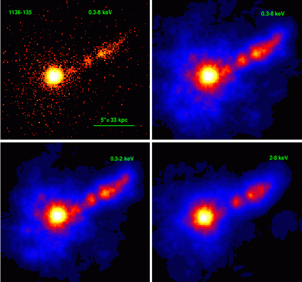
Figure 1: X-ray images of the jet of 1136–135 from a 77.4 ks Chandra ACIS-S exposure. Top, Left: raw ACIS image in total band. Top, Right to Bottom, Right: smoothed ACIS images in total, soft, and hard band, respectively. In the smoothed images, the pixel size is 0.1^′′. North is up and East to the left.

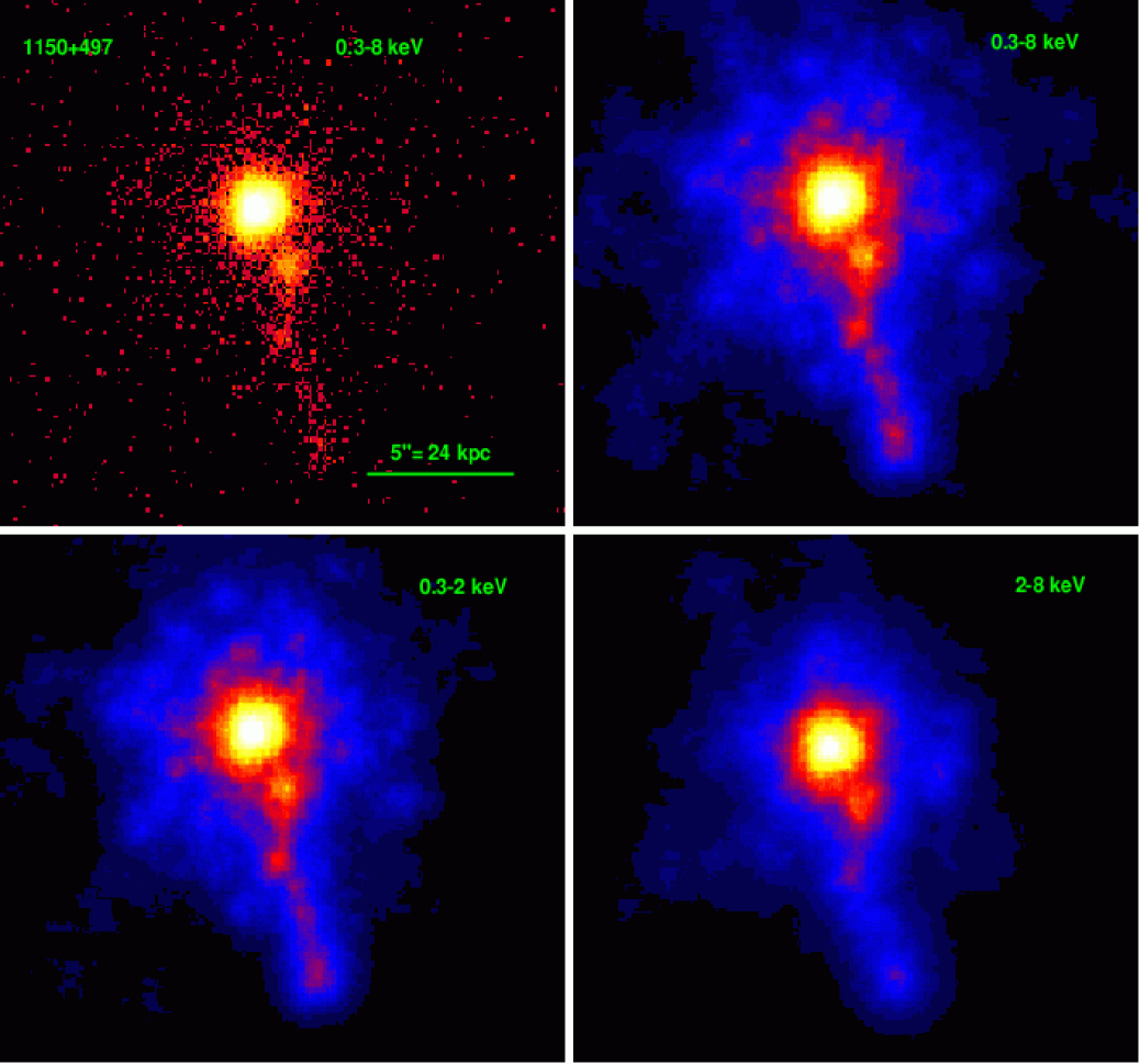
Figure 2: X-ray images of the jet of 1150+497 from a 68 ks Chandra ACIS-S exposure. Top, Left: raw ACIS image in total band. Top, Right to Bottom, Right: smoothed ACIS images in total, soft, and hard band, respectively. In the smoothed images, the pixel size is 0.1^′′. North is up and East to the left.

The Chandra data were reduced following standard screening criteria and using the latest calibration files provided by the Chandra X-ray Center. The latest version of the reduction software CIAO v. 3.1 was used. Pixel randomization was removed for imaging purposes only, and only events for ASCA grades 0, 2–4, and 6 and in the energy range 0.3–8 keV were retained. We also checked that no flaring background events occurred during the observations. After screening, the effective exposure times are 70.2 ks for 1136–135 and 61.7 ks for 1150+497. The X-ray images of the jets are shown in Figures 1 and 2, top-left panels while the X-ray count rates for the various knots are listed in Table 2.

Background spectra and light curves were extracted from source-free regions on the same chip of the source. For the jets knots the spectra were extracted from ellipses of axes in the range 0.5–1^′′, depending on knot’s size and location, centered on the position of the knot’s radio counterpart. An important issue, further discussed in § 4.3, is the presence of a non-zero basline in the X-ray emissivity profile of the jets (Figures 5 and 6). While some knots stand out clearly against this baseline (e.g., A in 1136–135 and E in 1150+497), most are fainter and blend with the surrounding regions. We thus used extraction regions of different dimensions for the various knots, depending on their FWHMs. In all cases, the size of the extraction region in both dimensions (parallel and perpendicular to the jet’s axis) is $\;\buildrel>\over{\sim}\;$the measured FWHM of the knot. The fluxes (but not the count rates) were corrected for the effects of a finite “aperture”.

The response matrices were constructed using the corresponding thread in CIAO 3.1. The ACIS spectra with $>$ 100 counts were analyzed in the energy range 0.5–8 keV, where the calibration is best known (Marshall et al. 2004) and the background negligible, and were grouped so that each new bin had $\geq$ 20 counts to enable the use of the $\chi^{2}$ statistics. The spectra were fitted within XSPEC v.11.2.0. Errors quoted throughout are 90% for one parameter of interest ($\Delta\chi^{2}$=2.7). The unbinned X-ray spectra with $<$ 100 counts were fitted using the C-statistics.

The 0.3–8 keV counts of the sources, extracted from the regions described above, are reported in Table 2 for each knot. Note that the counts were extracted from different-size regions for each knot. This was necessary to avoid overlaps in the extraction regions for contiguous knots at the limited Chandra resolution. Following the radio, elliptical extraction regions were used in the X-rays.

3.2 HST

Both 1136–135 and 1150+497 showed optical counterparts to their radio/X-ray jets in our earlier STIS images (S02, S04). In order to constrain the optical spectrum of the brightest optical features, we observed the two objects in three filters with the Advanced Camera for Surveys (ACS) aboard HST. The total exposures were one orbit for 1136–135, which has the brighter optical knots, and two orbits for 1150+497 which is relatively fainter. The central frequencies of the three filters, F475W (SDSS g), F625W (SDSS r), and F814W (broad I), are 6.32, 4.75, and 3.72 $\times 10^{14}$ Hz, respectively. Longer total integrations were obtained at the shorter wavelengths because of the expected steep spectrum nature of the jet emission. In the case of the F814W exposure of 1136–135, we received two consecutive segments of different duration each (338s and 182s).

The data were obtained from the STScI archive with pipeline processing applied. The pipeline implements the MultiDrizzle (Koekemoer et al. 2002) program to deliver calibrated and cosmic-ray cleaned images. Accurate photometry of the faint jet knots is limited by the high background levels due to sensitivity of the ACS to field sources, and contamination from the central sources, in the form of scattered light and prominent diffraction spikes from the bright quasar nucleus and diffuse emission possibly from the host galaxy. To isolate the jet knot emissions, we used square apertures centered on the X-ray/radio aperture positions. The elliptical apertures we defined for the Chandra/radio data are not practical to use due to the aforementioned contamination sources.

In the case of F814W images of 1136–135, the MultiDrizzle pipeline could not remove cosmic rays. Thus, we adopted the following procedure: we used the longer segment to remove the host galaxy’s contribution and to measure the jet fluxes. For knots C and D, where cosmic rays contaminate the extraction region for the fluxes, we used the shorter segment which was clear.

We estimated the background using identical apertures (9x9 image pixels) in adjacent regions to the extractions. Several background regions at different positions were used; since the background varies, we used the average and standard deviation of the values estimated in the boxes. The net flux was derived as the difference of the total flux minus the average background. As uncertainty on the net source flux, we used the error percentage defined as the ratio of the background standard deviation over the net source flux.

We claim detections in the cases where the net source flux is at least 3$\sigma$. For the non-detections, we quote 3$\sigma$ upper limits. Counts were converted to flux densities using the inverse sensitivity measurement given by the keyword PHOTFLAM in the image headers. Extinction corrections were estimated using values for the closest matching standard bands provided in NED (from Schlegel et al. 1998). These corrections ranged from a few up to 17$\%$ at the shortest wavelength. The fluxes in each filter are listed in Table 3 for each knot.

3.3 Radio

As part of our Chandra and HST survey (S02, S04) we obtained multi-band radio data for the jets which had X-ray and/or optical detections. Here, we use the new data obtained with the NRAO Very Large Array at 22 GHz, and with the MERLIN array at 1.7 GHz both achieving $\sim$0.15–0.3^′′ resolution. The 5 GHz VLA data were previously presented in our GO2 papers (S02, S04).

The new data are discussed in full elsewhere (Cheung 2004; Cheung et al. in preparation). Briefly, 22 GHz VLA data were obtained in 2002, May and July for 1136–135 and 1150+497, respectively, with integrations of about three hours on each target (1$\sigma$ rms $\sim$0.1 mJy/bm). The B-configuration was used for 1150+497 to achieve similar resolution to the 5 GHz, A-configuration image (Owen & Puschell 1984; Fig. 4). The 1136–135 observations utilized the hybrid BnA configuration to achieve a more circular beam on this low declination target. The MERLIN 1.7 GHz observations were obtained in Jan-Feb 2002 over several observing runs (rms $\sim$ 0.3–1.0 mJy/bm). Initial calibration was performed at Jodrell Bank by the archivists and the final imaging and self-calibration done at Brandeis.

In addition, a new full-track 8.5 hour, 8.4 GHz VLA observation (8 Nov 2003) of 1136–135 was obtained for the purpose of this work. This was necessary because the other radio images did not detect the inner ($<$5^′′) radio jet clearly whereas the Chandra image did. The on-target time was 7.7 hrs with the remaining time spent on calibrator sources. The resultant rms noise in the naturally weighted image is approximately 10$\mu$Jy, a few times what is expected from thermal noise, resulting in a very high-dynamic range image (Figures 3-4).

The radio fluxes for the jet regions were extracted using identical elliptical apertures to those used in the X-ray analysis. Errors in flux density are, conservatively, 10% for the brightest features, with larger values estimated for fainter features and the noisier (1.7 and 22 GHz) data. Fluxes are reported in Table 3.

The main purpose of our new deep VLA 8.46 GHz map of 1136–136 was to image/detect the faintest features in its jet (knots $\alpha$ and A). The emission from these knots were not well-detected in the other data (MERLIN 1.7 GHz, archival snapshot VLA 5 GHz, and new 22 GHz) and their fluxes would be underestimated from these maps. The knots, however, appear fairly well in our reprocessed VLA 1.5 GHz map from the Saikia et al. (1990) data and we were able to estimate their fluxes above the surrounding extended lobe emission. The fluxes are: 10.9 $\pm$ 1.6 mJy for knot $\alpha$, and 12.1 $\pm$ 1.8 mJy for knot A. Using these fluxes, and those at 8.46 GHz, the radio energy indices were derived for these two knots. They are consistent with those measured for the brighter regions of the jet (Table 3). The radio fluxes of knots $\alpha$ and A at 5 GHz and 22 GHz reported in Table 3 were extrapolated assuming these energy indices and the 8.46 GHz flux.

4 Results

4.1 Imaging

Figures 1-2 show the Chandra images of 1136–135 and 1150+497, respectively. The top-left panel is the ACIS-S raw image in the total energy range 0.3–8 keV, with no smoothing applied. The remaining panels show the smoothed ACIS-S images in total (0.3–8 keV), soft (0.3–2 keV), and hard (2–8 keV) X-rays. The ACIS-S images were smoothed using the sub-package fadapt of FTOOLS with a circular top hat filter of adaptive size in order to achieve a minimal number of 10 counts under the filter. The faint horizontal streak originating from the cores is the readout streak, caused by out-of-time events from bright point sources (cores).

The multiwavelength images are presented in Figures 3-4, where the smoothed 0.3–8 keV ACIS and the HST ACS images are illustrated with the 8.46 GHz (1136–135) and 4.9 GHz (1150+497) radio contours overlaid. The optical images are from the F625W filter because of its higher signal-to-noise ratio and the lower contamination from cosmic rays, which could not be removed automatically. Optical emission is present from several of the X-ray and radio knots; the chance probability that the optical features are due to the coincidental superposition of background stars or galaxies is $\;\buildrel<\over{\sim}\;$$2\times 10^{-3}$ for 1136–135 and $\;\buildrel<\over{\sim}\;$$3\times 10^{-3}$ for 1150+497, while the combined X-ray/optical probabilities are $\;\buildrel<\over{\sim}\;$$10^{-5}$ and $10^{-6}$, respectively. Also shown in Figures 3-4 are the 22 GHz radio images. While confirming all the previously detected features, the observations reveal important new details on the jets structure, as discussed below for each source.

To investigate the jet structure at X-rays we plot in Figures 5-6 the X-ray profiles of the jet. The latter were extracted from ACIS images after rebinning (factor 0.2, yielding pixel size 0.1^′′) and smoothing with fadapt with a threshold of 10 counts. For the extraction region we used a box of width 1.5^′′ and length equal to the jet length, or 9.4^′′ for 1136–135 and 7.6^′′ for 1150+497. The jet flux was collapsed on the central axis of the box. Shown in Figures 5-6 are the total 0.3–8 keV, soft (S) 0.3–2 keV, and hard (H) 2–8 keV jet profiles. The bottom panel shows the run of the softness ratios, defined as (S-H)/(S+H), along the jets. We stress that these profiles, and those in Figures 7-8, were derived to show the qualitative run of the fluxes along the jet. The uncertainties vary between 10% and 40% with the largest errorbars on the hard X-ray and softness ratio data. Overall, in both cases the jet emission profile consists of a non-zero baseline over which more or less defined peaks are superposed.

The jet profiles at X-rays (total band), optical (F625W), and radio (8.5 GHz for 1136–135, 4.9 GHz for 1150+497) are illustrated in Figures 7-8. No rebinning was applied to the radio and ACS data. For the radio profile we used the same extraction procedure as for the X-rays. However, for the optical profile multiple and narrower boxes were used, to follow the jet bending and to limit the background contamination. The horizontal dotted lines mark the background; the contribution of the core PSF wings dominates the background in the inner parts (not plotted). For the optical data, as the background varies depending on position, we plotted an average value. However, a few features which appear in Figures 7-8 to be above the plotted background are in reality only upper limits, due to a higher local background. These are marked by vertical arrows.

The vertical dashed lines in all panels mark the position of the knots. A word of caution is necessary in this regard. Only a few X-ray features stand out clearly and all correspond to well defined radio features. Towards the end of the jets the X-ray emission appears more diffuse and the positions of the radio features were used to mark the knots in Figures 7-8. However, in some cases the radio knots do not have clear counterparts at the shorter wavelengths (e.g., knot G in 1150+497, see below). In the the jet of 1150+497 the knots appear less prominent than in 1136–135 and individual fainter knots in the jet profiles cannot be resolved unambiguously.

Also listed in Table 2 are the FWHM of the X-ray knots in the direction orthogonal to the jet’s axis and in the energy range 0.3–2 keV. The latter were extracted in the softer part of the energy range where the PSF is better described and less energy-dependent (Karovska et al. 2001). To measure the FWHM of the knots we used the rebinned and smoothed ACIS-S images described above. The knot profile in the direction orthogonal to the jet’s axis was extracted by collapsing the counts into a narrow slice of dimensions 1^′′$\times$3^′′ (projection in ds9). Then, the FWHM of the gaussian-like distribution of the counts was estimated simply by measuring the width at half maximum. For the PSF, we used the core image and followed the same procedure to extract the profile of the point-like core. Note that weak diffuse X-ray emission around the cores is present (Sambruna et al. 2005, in prep.); however, the extended emission around the core becomes non-negligible after a radius of 5^′′. Thus, the PSF was measured inside 3^′′ and it is not affected by the diffuse emission. The comparison between the PSF and the knot’s profile was used to gauge whether the knot was resolved.

In Table 2 the uncertainty on the FHWMs is $\;\buildrel>\over{\sim}\;$0.1^′′, which is the size of the pixel in the images. Also listed is the difference in quadrature between the PSF FWHM (0.6^′′) and the knots’. From Table 2 it can be seen that, assuming a minimum uncertainty of 0.1^′′, only knots $\alpha$ and A in 1136–135, and knots B, C, and E in 1150+497 are only slightly resolved at 1$\sigma$. Similar results are obtained for profiles extracted in both soft (0.3–2 keV) and hard (2–8 keV) energy bands.

To evaluate the FWHM of the knots in the direction along the jet, we fitted the knots profiles in Figures 5 and 6 with Gaussians. Ideally, these profiles should be compared to the core’s; in practice, the presence of non-zero faint emission in between the knots hampers this comparison. In addition, this procedure can only be performed for the isolated knots – i.e., knot A for 1136–135 and knot E (at soft X-rays) for 1150+497. Both knots are unresolved in the direction parallel to the jet.

We now comment on the results for the jets of the two sources separately.

4.1.1 1136–135

Figures 1 and 3 show that all the X-ray features detected in the short exposure (S02, S04) are confirmed in this longer observation. However, more detail is hereby revealed at the larger signal-to-noise ratio of the ACIS data.

The innermost part of the jet at 2^′′ from the core (knot $\alpha$ in S04) is clearly visible. As apparent from Figure 1, knot $\alpha$ is more prominent at soft X-rays where it is composed of a faint stream of emission emanating from the core and terminating in a more diffuse knot. There is a possible optical counterpart in the HST image (Figure 3), which is clearly detected only after an appropriate galaxy subtraction. At radio wavelengths, knot $\alpha$ is detected at 4.9 and 8.5 GHz.

Knots A and B discussed in S02 are confirmed and resolved (Table 2). Here knot B appears to be more complex than a single feature, with possible substructures, especially at soft X-rays (Figures 1 and 5). Unfortunately, the two substructures are too small (radii $<$ 1^′′) preventing a meaningful analysis; in Table 2 and 3 we quote the total X-ray flux from knot B. The count rate is 0.0028 c/s, slightly smaller than 0.005 c/s quoted in S04. The discrepancy is probably due to the smaller extraction radius used here ($\sim$0.7^′′) compared to 1^′′ used in S02, S04.

Three new X-ray features are identified in the deep ACIS image: knots C, D, and E at 7.7^′′, 8.6^′′, and 9.6^′′, respectively (Table 2). Knots C and D have optical counterparts (Figure 7 and Table 3). The final part of the jet, hotspot HS at 10.3^′′, was formerly known as “knot C” in S02, S04.

Inspection of the jet profiles in Figures 5 and 7 shows that there is a generally good correspondence between knots at the various wavelengths, but with a few notable exceptions. First, concentrating on the soft and hard X-ray profiles, knot $\alpha$ is more pronounced at soft X-rays and barely present at harder energies. Similarly, knot C and D disappear in the hard X-ray band, while a new component emerges in between them at $\sim$ 8^′′. Interestingly, for knot A there is an offset of $\sim$ 0.4^′′ ($\sim$ 2 kpc projected size) between the soft and hard X-ray peaks, with the softer energies further downstream than the hard X-rays. However, the position of the X-ray knot in the total band aligns well with the optical and radio peaks (Figure 7).

Another note of interest is the presence of non-zero inter-knot X-ray emission especially in the inner portion of the jet (see below). While it is possible that the fainter inter-knot emission observed in some X-ray jets (Chartas et al., 2000; Schwartz et al. 2000; Marshall et al. 2001; S04) is actually due to unresolved faint features, very weak diffuse emission cannot be excluded. This is discussed in § 4.2.

Also interesting is the overall structure of the jet at the three wavelengths - X-rays, optical, and radio. Figure 7 shows a qualitatively different jet behavior before and after knot B, the most prominent feature at the shorter wavelengths. In the X-rays, upstream of knot B the jet is mainly composed of discrete, isolated peaks, while downstream of knot B the X-ray emission cascades with “continuous” emission and a few faint knots superposed. The radio profile shows a different behavior. At these wavelengths knot B is barely discernible, while knots $\alpha$ and A are detected, but faint. The radio profile increases steadily downstream from knot B and peaks at the end of the jet, opposite to the X-ray profile. The optical profile is intermediate, consisting of isolated knots both in the inner and outer parts.

The multiwavelength profiles of the 1136–135 jet are strongly reminiscent of the 3C 273 morphology (Sambruna et al. 2001). In the latter jet, in fact, opposite trends between the runs of the X-ray and radio profiles were observed similar to the case of 1136–135. This led us (Sambruna 2001, S04) and other authors (Georganopoulos & Kazanas 2004) to suggest plasma deceleration as a cause of the observed decrease of the X-ray to radio ratio from the inner to the outer regions of the jet. We will discuss this scenario more quantitatively in Paper II.

4.1.2 1150+497

This jet has an interesting wiggling morphology. All the detected features from S02 are confirmed.

The innermost radio knot A can not be detected even at optical wavelengths where it is covered by the core PSF. The brightest detected and resolved feature at both X-rays and optical is knot B at $\sim$ 2^′′. It appears complex especially at soft X-rays, where it exhibits a faint arc-like structure to the South, ending in knots C+D (Figure 2). Radio knot E, not previously seen at X-rays, is now weakly detected and appears to be soft. Similarly, knots F and G, and hotspot H, previosuly detected in the short GO2 exposures (S04), are confirmed.

Figure 6 displays the X-ray jet profiles in the soft and hard bands, while the total X-ray, optical, and radio profiles are shown in Figure 8. Overall, the run of the flux along the jet is similar at all wavelengths, in contrast to 1136–135. The two most prominent knots, B and E, and the terminal part of the jet, IJ, show a rough 1:1 correspondence between the X-rays, optical, and radio. Knots C and D are visible mainly at X-rays and optical (D). For knot G, the vertical dashed line traces the position of the radio knot; no feature is present at X-ray and optical at the radio position. However, there are possible counterparts located $\sim$ 0.5^′′ and $\sim$ 0.3^′′ upstream of the radio position at X-rays and optical, respectively.

Another interesting feature of the multiwavelength profile is the sudden increase of the radio emission at the end of the jet. A more modest rise is present at X-rays. This behavior is qualitatively similar to that of 1136–135 though on a smaller angular scale. If the terminal feature of this jet is interpreted as a hot-spot in the lobe, plasma deceleration is again plausible (see discussion in § 5.2).

4.2 Spectral Analysis

X-ray spectra: The X-ray spectra were fitted with a single power law plus Galactic absorption model, which provided generally a satisfactory fit to the data. The results of the spectral analysis are reported in Table 2, where the photon indices, $\Gamma_{X}$, and 90% uncertainties are listed. (The photon index is related to the energy index as $\Gamma_{X}=\alpha_{X}+1$.) The aperture-corrected 1 keV flux densities are reported in Table 3, together with the fluxes from the other wavelengths.

In 1150+497, the X-ray slopes are similar for all the knots, $\Gamma_{X}\sim 1.5-1.7$. In 1136–135, the fitted photon indices for the brightest X-ray knots $\alpha$, A, and B are relatively steep, $\Gamma_{X}\sim 2.0$, although the uncertainties are large. The photon index for knot B is marginally ($\;\buildrel<\over{\sim}\;$2$\sigma$) consistent with the value previously quoted in S04, $\Gamma_{X}=1.5\pm 0.5$. The discrepancy is due to the larger extraction radius used in S02, S04, which includes a contribution from the following knot C, previously unidentified. In fact, the measured X-ray slope of knot C at 7.7^′′ is $\Gamma_{X}\sim 1.5$, flatter than in knot B. For the remaining knots C, D, E, and the hotspot HS the X-ray slopes are affected by large uncertainties.

Additionally, we fitted the brighter knots’ X-ray spectra with a thermal bremmstrahlung and a composite model consisting of the thermal bremmstrahlung plus a power law. The fits with the thermal or thermal + power law model are significantly worse than the single power law, and/or yield unphysical values for the temperature/photon index.

The 1 keV flux densities listed in Table 3 were derived using the photon indices from the spectral fits. For the weak knots with $<$ 100 counts, however, we calculated the fluxes from the counts in Table 2 assuming $\Gamma_{X}=1.8$ plus Galactic column density for both sources. These are fully consistent with the fluxes calculated using the slopes in Table 3, which are affected by large uncertainties.

We further investigated X-ray spectral variations along the jets by means of softness ratio profiles, as shown in the bottom panels of Figures 5-6. The softness ratios are defined as SR=S-H/(S+H), where S are the counts in the energy band 0.3–2 keV and H the counts in 2–8 keV. As seen in Figures 5-6, X-ray spectral variability is clearly present along the jets. In both sources, a trend is apparent of softer X-ray spectra at the knot positions than in the inter-knot regions, however, as stated above the uncertainties are large.

The core X-ray spectra exhibit interesting properties, which will be presented in a future publication.

Optical spectra: Table 3 lists the dereddened optical fluxes for the detected knots in the various filters. Upper limits are reported for the non-detections. Note that some knots have a firm detection in only one or two filters.

To derive the optical slopes, we performed a linear fit to the fluxes in Table 3. To take into account the optical upper limits for some of the knots, we used the ASURV statistical package. However, no reliable estimate of the optical slope was obtained, given the small number of datapoints available to begin with.

Thus, we only considered knots for which firm detections in at least two filters are present. The slopes derived from a linear interpolation of the optical fluxes are listed in Table 3. No uncertainties are listed for the knots with only two detections, as errors in these cases are meaningless. While we report the derived slopes also for the faintest optical knots (marked in Table 3), these values should be regarded with caution due to the lower signal-to-noise ratio of the data.

Radio spectra: Also listed in Table 3 are the radio energy indices, derived from a linear interpolation to the available radio data (see § 3.3). The average index is $\alpha_{rad}=0.7$ for both jets. Interestingly, the radio spectral indices are comparable to the X-rays slopes in the cases of knots $\alpha$, A, B, C, and D for 1136–135, and all knots for 1150+497. This is expected if the same population of very low energy electrons is responsible for scattering the CMB photons into the X-ray energy band.

4.3 Residual X-ray emission around the knots

In S04 we noted the presence of faint residual X-ray emission in between the knots in several jets. Emission from the inner jet was also detected in PKS 0637–752 in a 100 ks ACIS-S exposure (Chartas et al. 2000, Schwartz et al. 2000), in 3C 273 (Marshall et al. 2001), and in the M87 jet (Perlman & Wilson 2005).

As shown by visual inspection of Figures 1-2, faint X-ray emission seems to be present between the knots in both the jets of 1136–135 and 1150+497. This is confirmed more quantitatively by the jet profiles in Figures 5-6 which show a non-zero baseline in between the individual emission peaks, above the ACIS background. For easiness of reference, we will call this residual X-ray emission “inter-knot”.

We extracted the spectrum of the inter-knot X-ray emission, by subtracting the knots’s contribution from the total jet spectrum. The extracted spectrum, with a total of 241 and 326 counts for 1136–135 and 1150+497, respectively, represents the total inter-knot X-ray emission. In the assumption that the emission has the same origin everywhere throughout the jet (an oversimplistic assumption), the X-ray spectrum obtained with this procedure was fitted using a thermal bremsstrahlung and a power-law models.

Despite the relatively large number of counts the spectra are quite noisy, warranting the use of the C-statistics in the spectral analysis. The noiseness of the spectra could be related to the large extraction region, encompassing a wide physical region of the jet where multiple emission mechanisms and/or parameter gradients could be present. From the fits, we find that it is not formally possible to distinguish between a thermal and non-thermal origin of the X-ray emission from the inter-knot region in 1150+497: both the bremmstrahlung and a power-law models represent the data adequately in this jet. In the case of 1136–135 the bremmstrahlung is better ($\Delta$Cstat=10 for same d.o.f.s) than the single power law. The fitted temperature is very similar in both sources, $kT=2.7^{+1.4}_{-1.0}$ keV for 1136–135, and $kT=2.7^{+1.7}_{-0.7}$ keV for 1150+497. The power-law photon indices are $\Gamma_{x}=1.6^{+0.5}_{-0.1}$ for 1136–135, and $\Gamma_{x}=1.9\pm 0.2$ for 1150+497. The observed 0.3–8 keV fluxes are $1.6\times 10^{-14}{\rm~{}erg~{}cm^{-2}~{}s^{-1}}$ and $2.8\times 10^{-14}{\rm~{}erg~{}cm^{-2}~{}s^{-1}}$ for 1136–135 and 1150+497 respectively, and the corresponding intrinsic luminosities are $3.1\times 10^{43}{\rm~{}erg~{}s^{-1}}$ and $1.3\times 10^{43}{\rm~{}erg~{}s^{-1}}$.

The origin of the inter-knot X-ray emission is not clear. A first possibility includes thermal emission from shocked ambient gas as the plasma plows its way through the ISM. However, there is no evidence of such extended emission in the radio images, where the knots appear elongated in the direction of the jet’s axis (Figures 3 and 4). Another argument against thermal emission is the lack of rotation measure in the radio (§ 5.3).

An alternative scenario is that the faint inter-knot X-ray emission is due to unresolved features (e.g., oblique shocks or a population of hot electrons, see § 5.3), or simply are due to our definition of “knot”, forcefully arbitrary and resolution-dependent. Indeed, on one side in order to quantify their emission we are forced to assume a finite size for the knots ($\;\buildrel>\over{\sim}\;$the PSF size); on the other, it is unlikely that the physical emission region is intrinsically well defined, for example due to particle diffusion and escape, or spatial and/or temporal inhomogeneities. A related problem is the faintness of the emission at the end of the jet, where the emission peaks are less well separated from each other (Figure 5 and 6).

We conclude that there is evidence for the presence of unresolved X-ray emission around the knots in the jets of 1136–135 and 1150+497. Its nature (unresolved features vs. truly diffuse emission) is unknown. Possible interpretations are discussed in § 5.3.

4.4 Spectral Energy Distributions

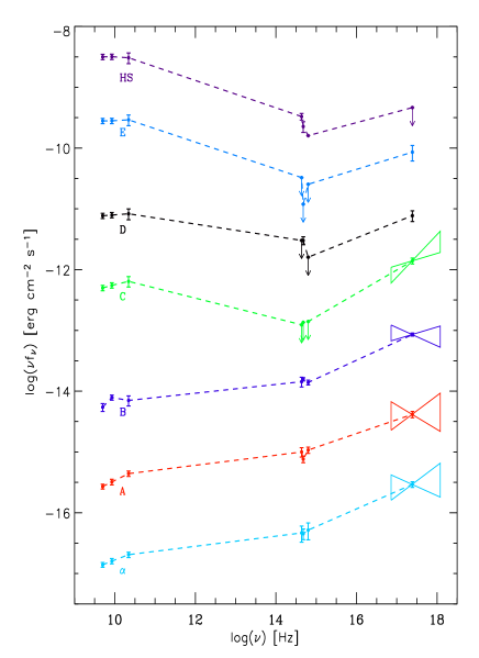
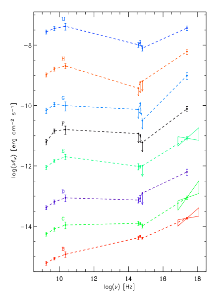
Figure 9: Spectral Energy Distributions (SEDs) of the jets of 1136–135 (left) and 1150+497 (right). In each panel, going from bottom to top the SEDs are plotted from the inner to the outer jet, with arbitrary shifts for clarity. Spectral changes are observed in the jet of 1136–135, while the SED shape of 1150+497 remains fairly constant.

The Spectral Energy Distributions (SEDs) of the emission from the various knots are the basis to investigate the origin of the emitted radiation and the physical conditions in different regions of the jets. The SEDs of the knots are illustrated in Figures 9a-b, for 1136–135 and 1150+497 respectively. For clarity of presentation in each panel the SEDs were shifted arbitrarily to allow comparison of spectral variations along different locations in the jet. Going from bottom to top the SEDs run from the innermost to the outermost detected knot, including the terminal hotspots.

While some of the SEDs were already presented in S02 and S04, the deeper X-ray and optical and radio images have provided better information about the jets morphologies, with a few additional knots having been detected. Moreover, for the first time we are able to take advantage of additional constraints provided simultaneously by the optical and more accurate X-ray continuum slopes.

In the case of 1136–135, a spectral progression is clearly present. The radio-to-optical continuum steepens systematically from the innermost knot, $\alpha$, to the outermost one, E. The radio and optical continuum slopes also steepen, while the X-ray spectrum flattens. For the two innermost knots, $\alpha$ and A, the optical continuum appears to be flat. For knots B and C the optical spectra are steep, indicating a break between the X-rays and the longer wavelengths.

In 1150+497 there are less spectral variations. The radio-to-optical continuum steepens, however, no clear trend is present for the optical-to-X-ray continuum. Similarly, the radio and X-ray continua do not change significantly from the inner to the outer regions of the jet, with the X-rays maintaining a rather flat slope, inconsistent with an extrapolation of the optical data.

In order to quantify the above trends we derived broad-band spectral indices (Table 4). Using the 1 keV, 6250Å, and 5 GHz fluxes in Table 3, we derived the radio-to-X-ray, $\alpha_{rx}$, the radio-to-optical, $\alpha_{ro}$, and the optical-to-X-ray, $\alpha_{ox}$, spectral indices. Figures 10a-c show the plots of the two-band energy indices versus the distance from the core in both sources. In S04 we found that in all jets where multiwavelength information is available for multiple knots there is a trend of increasing radio-to-X-ray and radio-to-optical flux ratios with increasing distance from the core. Figures 10 show that this trend is confirmed for the jet of 1136–135, where both $\alpha_{rx}$ and $\alpha_{ro}$ increase steeply with core distance. No trend is observed for $\alpha_{ox}$ in this source. We recall that due to the larger uncertainties of the optical fluxes and to the shorter frequency range the latter index has larger errors.

For 1150+497 there are no demonstrable trends. A $\chi^{2}$ test gives negligible probability of variation, i.e., in all three cases the run of the energy index with core distance is consistent with a constant. Inspection of Figure 8, however, shows that while the X-ray emission fades systematically toward the end of the jet, the radio increases abruptly at the position of the terminal hotspot. This is likely related to a compression event that increases the synchrotron emissivity through an increase of the magnetic field and electron density (see § 5.1).

Inspection of the SEDs in Figures 9 shows that in all the knots the optical points lie below the line connecting radio and X-rays, indicating that a single power-law extending from the radio to the X-rays can not reproduce the overall SEDs. Moreover, the different slopes of the optical continuum suggest that the origin of the optical emission can be different in different knots. Steep optical slopes ($\alpha_{opt}$ $\;\buildrel>\over{\sim}\;$1) suggest that the optical emission belongs to the high-energy tail of the synchrotron radio component, while flatter slopes suggest that the optical belongs to the same spectral component responsible for the X-ray emission. In some knots (notably in knot A and B in 1136–135) the situation is quite unclear, since the slope is poorly determined. We refer to the next section for a quantitative discussion of emission models for representative knots.

In S02, S04 we showed that the jet of 1150+497 and the outer knots of the 1136–135 jet (C, D, E) had SEDs consistent with a model with two emission components: synchrotron emission at longer wavelengths, and Inverse Compton scattering of the CMB (IC/CMB) at higher energies, implying a relativistic jet on kpc-Mpc scales. The inner knots of 1136–135 ($\alpha$ and A in this paper) were instead consistent with synchrotron emission from radio to X-rays. The synchrotron interpretation was suggested by the fact that available radio, optical, and X-ray datapoints for $\alpha$ and A were consistent with a single power-law. The new data presented here question this interpretation, since the optical flux falls about a factor of 2 below the radio-to-X-ray extrapolation. This result highlights the importance of high quality data in studying multiwavelength emission from these structures.

5 Modeling the multiwavelength jet emission

5.1 Modeling the SEDs

We assume that the radio to X-ray emission from the knots of 1136–135 and 1150+497 is produced through synchrotron and IC/CMB scattering from a relativistic electron population with a power law energy distribution. We include the terminal knot in the analysis. Whether this correspond to the traditional hotspot (Bridle et al. 1994) is an open question in this case. As shown in Tavecchio et al. (2005b), there is compelling evidence that, as originally suggested by Georganopoulos & Kazanas (2003), the emission from these portions of the jet, usually considered at rest, is produced by plasma still in motion with mildly relativistic speeds ($\Gamma\sim 2-3$). The advancement speed of the terminal shock front, however, can be subrelativistic.

We refer to Tavecchio et al. (2000) and S02 for a full description of the model used to reproduce the jet emission. Briefly, the emitting regions are assumed here to be ellipsoidal, with volumes $V$ corresponding to the flux extraction regions used above (§ 3). We assume that the emitting region is in relativistic motion, with Doppler factor $\delta$ and homogeneously filled by high-energy electrons, with a power-law energy distribution $N(\gamma)=K\gamma^{-n}$ extending from $\gamma_{\rm min}$ to $\gamma_{\rm max}$. Electrons radiate via the synchrotron and IC/CMB mechanisms. The low-energy limit of the electron distribution $\gamma_{\rm min}$ is well constrained by the condition that the low-energy part of the IC/CMB component should not overproduce the observed optical flux. To close the system of the model parameters we assume that the energy densities of relativistic electrons and magnetic field are in equipartition (protons are not included, i.e. $k=0$ in the standard notation). This closely corresponds to the minimum energy condition.

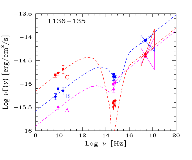
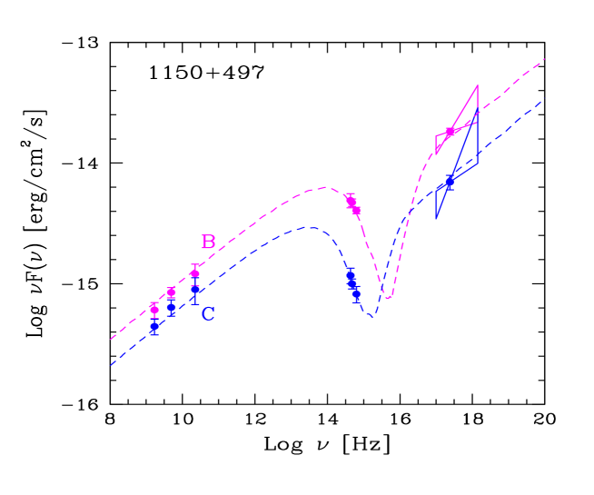
Figure 11: Spectral Energy Distributions for selected knots in the jets of 1136–135 (top) and 1150+497 (bottom). The lines are fits with the synchrotron+IC/CMB model (see text). Note how the optical slope is critical to determine whether the optical emission is due to synchrotron or is the low-energy tail of the IC/CMB component.

Specific models for different representative knots are discussed in the following. The computed emission models are shown in Figures 11a-b together with the observational data points.

For 1136–135 we consider first knots A and B which were detected in all the three optical bands. The present data for knot A suggest a moderately concave SED with the optical fluxes falling below the radio to X-ray connection by a factor of about 2. Note that the radio flux associated with this knot was revised upwards by a factor 5. At the same time the optical slope is rather flat (though with large uncertainty) indicating a connection of the optical to the X-ray component. The emission model we computed attributes the optical emission mainly to the low energy tail of the IC/CMB, plus some contribution from the high frequency extension of the synchrotron component. Previously this knot was interpreted as a pure synchrotron knot. For knot B the situation is similar to knot A but the optical ”deficiency” is larger and the optical slope steeper. Here the model interpretes the optical fluxes as the synchrotron emission with a minor contribution from the IC/CMB. For comparison, we show in Figure 11a the spectral model for knot C. Here the optical upper limits separate the two components without ambiguity.

For 1150+497 we show in Figure 11b the spectral models computed for knots B and C for which there is good optical information. In both cases the optical slopes are steep suggesting a synchrotron origin of the optical emission. Note that for knot B the flux level of the optical emission falls close to a single power-law connecting the radio and X-ray fluxes. The optical slope is crucial to determine the model.

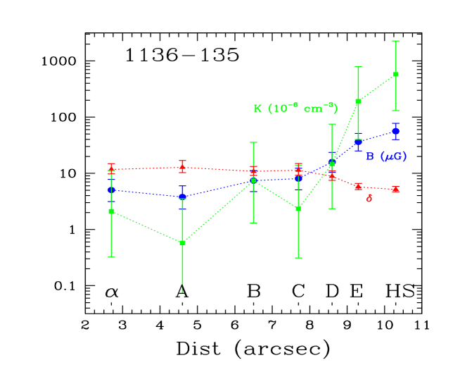
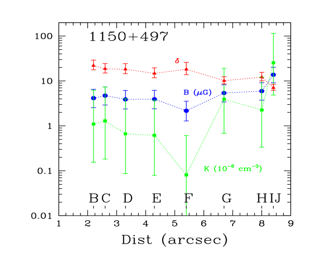
Figure 12: Plot of the Doppler factor $\delta$, magnetic field B, and electron normalization K along the jets of 1136–135 (top) and 1150+497 (bottom). The knots positions are labeled. The parameters were derived by fitting the IC/CMB model to the jet SEDs (see text). In 1136–135 the parameters vary along the jet; we interpret this as evidence for jet deceleration (see Paper II). In 1150+497, while the Doppler factor does not change, K and B increase at the end of the jet at the hot-spot location.

Computing spectral models for all the knots with sufficient data, we derived interesting parameters for different emission regions along the jets, such as magnetic field $B$, the normalization of the electron density $K$, the Doppler factor $\delta$. These are shown in Figures 12a-b as a function of projected angular distance from the core. To determine the uncertainty associated to each derived quantity we allow the input parameters to vary within a fixed range (5–25 for $\gamma_{\rm min}$, $V-V/2$ for the volume), while for the radio flux, the X-ray flux, and the radio slope we considered the errors reported in Table 3. We find that the uncertainty associated to the slope of the radio spectrum (directly related to the index $n$ of the electron energy distribution) largely dominates the final uncertainties, reported by the the errorbars in Figures 12a-b. We believe that the uncertainties estimated in this way are safely conservative, supporting the reality of any variation af the parameters along the jet.

Inspection of Figures 12 shows a clear difference between the profiles of the physical parameters of the two jets. For 1136–135 a systematic trend of all the parameters along the jet is apparent, in the sense of increasing $K$ and $B$ and decreasing $\delta$. For 1150+497 the profile is initially consistent with constant values along the jet for a large part of its length, while only at the end (close to the terminal HS) there is a significant increase of magnetic field, electron density and a decrease of the Doppler factor. Interestingly, the parameters estimated for the hotspot of 1136–135 are in good agreement with the trend followed by all the previous knots, supporting the idea that the so called ”hot spot” is connected to the jet flow.

5.2 Jet Deceleration?

One of the most striking differences between the two jets analyzed in this work is related to the jets radio and X-rays morphologies. Indeed, while the jet of 1150+497 presents a more or less similar fading trend at all three wavelengths up to the terminal hotspot, the jet of 1136–135 dramatically increases its radio luminosity after knot B while the X-ray emission rapidly fades. The different brightness profiles directly translate in the different run of the physical quantities from the SED modeling (Figures 12). In 1136–135, the increasing radio brightness requires an increase of the order of a factor 10 of the magnetic field and of the density of the radiating electrons, bound together through the equipartition condition. The decrease shown by the X-ray flux implies a decrease of the Doppler factor, which reduces the IC/CMB emission. Therefore, our analysis suggests that the observed morphology and multiwavelength profiles of the 1136–135 jet could be the result of a progressive deceleration of the emitting plasma flow after the region corrisponding to knot B–C.

This conclusion, already indicated by our analysis of the jet of 3C 273 and of the multiwavelength properties of our jet sample (Sambruna et al. 2001, S04), lends support to the model recently proposed by Georganopoulos & Kazanas (2004) for the deceleration of the jet plasma on kpc scales. In their analytical treatment the jet is supposed to decelerate adiabatically, with an associated increase through compression of the magnetic field and the particle density. These effects lead to an increase of the synchrotron flux, while the X-ray flux, produced through IC/CMB, decreases due to the diminishing importance of beaming of the CMB photons.

A discussion of the the most important physical consequences of the deceleration scenario will be presented in a companion paper (Paper II). Here we just comment briefly on two of them.

In Paper II, we discuss entrainment of external gas as a possible cause of the plasma deceleration in 1136–135 downstream of knot B. Indeed, from the analysis of the ACIS images of the cores we find evidence for the presence of circumnuclear hot gas in both sources on a scale of several tens of kpc. Moreover, X-ray observations show that low redshift ($z<1$) QSOs lie in environment typical of small groups (Hardcastle & Worrall 1999, Crawford & Fabian 2003). In the case of 1150+497, deceleration seems to occur on a shorter (projected) length and therefore is less apparent. Nevertheless, the possible scale length in terms of distance from the core is of the same order.

A second interesting aspect of the deceleration model of Paper II is that most of the ordered kinetic energy of the jet is converted during the deceleration into internal random kinetic energy of protons, increasing the total jet pressure. Only a small fraction of this energy can be transmitted to the relativistic electrons, since the inferred energy content in the relativistic electrons is limited to 10% of the dissipated energy. Comparing the radiative luminosity with the kinetic energy flux the overall efficiency is very small, $10^{-4}$–$10^{-3}$.

5.3 Inter-knot X-ray emission

The detection of residual inter-knot X-ray emission is particularly interesting in light of the deceleration scenario. We recall that the spectral fits of the jet are consistent both with a hot (2–3 keV) thermal component or with a non-thermal power law.

The first possibility to be considered is that the emission is produced by hot shocked plasma surrounding the jet (e.g., Komissarov 1994). In this case, we would expect values of the gas rotation measure from the radio in excess to the Galactic value. To constrain the rotation measure in the 1136–135 jet, we made use of our 4.86 and 8.46 GHz VLA polarization images, along with our recalibration of an archival 1.49 GHz VLA dataset published by Saikia et al. (1990). We measure a rotation measure in the jet consistent with the integrated galactic origin value of -26 $\pm$ 1 radians m^-2 (Simard-Normandin et al. 1981). Thus, we conclude that a thermal origin of the diffuse inter-knot emission in the 1136–135 jet is highly unlikely.

As anticipated in § 4.3, the residual inter-knot X-ray emission could be due to non-thermal emission from unresolved features associated to the knot, spatially and/or physically. Among these possibilities is that we are observing non-thermal emission produced by relativistic electrons accelerated in a thin boundary layer around the jet. In the model discussed by Stawarz & Ostrowski (2002) the competition between acceleration and radiation losses leads to a piled-up distribution, whose peaked synchrotron emission can be quite hard (up to $\nu^{1/3}$). The emission is most likely at X-rays: the peak energy is given by $E=0.9V_{8}$ keV, where $V_{8}$ is the characteristic velocity of the magnetic turbulence expressed in units of $10^{8}$ cm s^-1, expected to be of the order of the Alfven velocity, $V_{A}\sim 2\times 10^{8}$ cm s^-1 for typical parameters of the boundary layer. Thus, the faint interknot X-ray emission observed in the sources of this paper and others (S04) could be the synchrotron emission of hot electrons piled-up in the jet boundary layer.

6 Discussion

The previous discussion of the emission properties is based on the synchro-IC/CMB model and a number of assumptions. In the following we discuss some of the uncertainties and the theoretical problems associated with this interpretation.

One necessary caveat regards the fluxes used to construct the SEDs and the associated sizes of the emitting regions. We have already discussed the arbitrary definition of “knot” in § 4.3. Here we comment on the physical implications of using a given finite region size to extract the fluxes. Indeed, since images have different angular resolution at different frequencies, we are forced to measure fluxes using a quite large ”aperture”. However, the majority of the optical features detected in the jets appear to be smaller than the extraction regions. Therefore, we cannot exclude the possibility that the size of the emission region is frequency-dependent. It is conceivable that electrons are accelerated in a small volume and subsequently diffuse from the acceleration site, radiatively cooling: the high-frequency, optically emitting electrons will cool rapidly, while radio and X-ray electrons, characterized by a small energy, could diffuse into a larger volume. In this sense the use of a single extraction region and a unique volume in the modeling could be misleading.

Another important problem, related to the previous one, concerns the nature of the emission regions (see also Stawarz et al. 2004). In the modeling, the emitting region is assumed to be a ”blob” of plasma, in relativistic bulk motion. This is a reasonable assumption for many of the observed knots, visible as isolated spots within the jet (e.g., A in 1136–135). On the other hand, the morphology of 1136–135 after knot B where it is difficult to define knot and interknot regions suggests that a scenario considering emission from a continuous flow may be more realistic (Paper II). We note that the possibility that discrete knots mark portions of the jet characterized by larger density and/or speed with respect the average jet could help to overcome the difficulty regarding the large power requirement of IC/CMB jets, pointed out by Dermer & Atoyan (2004). In this case, indeed, the average power of the jet, stored in the lobes, could be significantly less than the “istantaneous” power inferred in the knots.

The above results were derived assuming that synchrotron+IC/CMB is the mechanism responsible for the radio-to-X-ray emission in both jets. Varius alternatives have been proposed in the past to explain the peculiar shape of the SEDs of knots: proton synchrotron emission (Aharonian 2002), synchrotron emission from a non power-law electron distribution (resulting from cooling, Dermer & Atoyan 2002, or from acceleration effects, Stawarz et al. 2004), synchrotron emission from two electron populations (Atoyan & Dermer 2004). Among these models, those invoking synchrotron emission from suitable electron distributions are the most promising.

In the model proposed in Dermer & Atoyan (2002), the underlying electron population is characterized by an energy spectrum which differs from the widely considered power-law form. The electron energy spectrum derives from cooling of a power-law distribution extending to large Lorentz factors (up to $\gamma\sim 10^{8}$). The cooling mechanism is Inverse Compton on the CMB, which for high-energy electrons is reduced because of the decline of the Klein-Nishina cross-section. As a consequence the derived spectrum is characterized by a “bump” at high energies. The synchrotron spectrum produced by such a distribution can reproduce the X-ray ”excess” characterizing some of the observed jets. However, as discussed in Atoyan & Dermer (2004), the model can not explain the emission from knots with steep optical spectra or knots in which the X-rays are much more luminous than the optical, even assuming quite extreme values for the parameters. For these cases the authors propose a two-component synchrotron model. Except for the innermost knots of 1136–135, most of the knots analized here exhibit a pronunced “concave” SED, for which the Dermer & Atoyan (2002) model can not be applied. The model proposed by Stawarz et al. (2004) encounters a similar difficulty.

Another uncertainty of the model is associated to the use of the equipartition condition in deriving the physical parameters of the knots. Stawarz et al. (2005) recently showed that, for the specific case of knot A in the jet of M87, the present upper limits on the SSC emission at high energy suggest a deviation from equipartition condition, with the magnetic field dominating the total energy. A possibility to explain such large magnetic field is that it is amplified by dynamo effects induced by turbulence. However, the present knowledge of this problem is still rather poor. Note that, relaxing the equipartition hypothesis, allowing for a dominance of the magnetic field (electrons), leads to larger (lower) values of the beaming factor. Moreover, the carried power will increase out of equipartition.

Clearly, several uncertainties and open questions remain in our understanding of the multiwavelength emission of large-scale jets. However, we believe that a simplified approach based on “individual” emission regions and equipartition is useful, as it leads to an unambiguous derivation of the physical conditions which can then be confronted with independent constraints.

7 Summary

We have presented deep Chandra ACIS and multi-color HST ACS observations of the jets of two powerful quasars, selected from our previous X-ray and optical survey (S04). The exposures and choice of filters for the ACS were optimized to obtain more detailed jet morphologies as well as X-ray and optical spectra for individual bright knots. The following results were obtained:

• All the jet features previously detected at X-rays and optical are confirmed. A few faint knots were detected for the first time, illustrating the importance of deeper exposures to gain a better knowledge of the jet structure.

• The jet profiles at the various wavelengths show in general good correspondence among the knots. A qualitatively different jet profile was observed in the two sources. In 1136–135, the jet X-ray emission fades after the most prominent knot B while the radio emission simultaneously increases. In 1150+497, the emission at all wavelengths steadily decreases, with the exception of the radio flux which increases again in the terminal jet region.

• The optical data indicate steep optical spectra in agreement with the expectations from the IC/CMB model, except for the first two knots of 1136–135.

• Large spectral variations are observed along the jet of 1136–135. Here, $\alpha_{rx}$ and $\alpha_{ro}$ steepen with distance from the core, and $\alpha_{ro}$ steepens with increasing radio luminosity of the knots.

• The multiwavelength morphology and SED variations in 1136–135 are consistent with the idea that the plasma suffers substantial deceleration on kpc-scales, as previously suspected for 3C 273 and other jets. A physical model is discussed in Paper II.

• The X-ray emission profile of the jets consists of a non-zero baseline over which more or less defined peaks are superposed. The origin of the non-zero inter-knot X-ray emisison is unclear, but a strong possibility consistent with the present data is non-thermal emission from unresolved features, such as oblique shocks or hot electrons piled-up in the jet boundary layer (Stawarz & Ostrowski 2002).

Table 1: The Targets
Source	$z$	Gal NH	logP${}^{5~{}GHz}_{core}$	logP${}^{5~{}GHz}_{jet}$	$R_{i}$	mV	log LBLR	log L[OIII]
(1)	(2)	(3)	(4)	(5)	(6)	(7)	(8)	(9)
1136–135	0.554	3.5	33.73	33.69	0.30	16.1	45.37	43.86
1150+497	0.334	2.0	34.53	34.95	2.3	17.1	45.80	43.75

Explanation of Columns: 1=Source IAU name; 2=Redshift; 3=Galactic column density in $10^{20}$ cm^-2; 4=Log of the core power at 5 GHz (in erg s^-1 Hz^-1); 5=Log of the jet power at 5 GHz (in erg s^-1 Hz^-1); 6=Ratio of core to extended (total-core) radio power at 5 GHz, corrected for the redshift (observed value times (1+z)); 7=Core optical V magnitude; 8=Total luminosity of the BLR (Cao & Jiang 1999); 9=Luminosity of the [OIII] line (Cao & Jiang 1999).

Table 2: X-ray Observations
Knot	Dist	FWHM	$\Delta$ FWHM	Counts	$\Gamma_{X}$	Opt?
	(′′)	(′′)	(′′)
1136–135
$\alpha$	2.7	0.75	0.45	98$\pm$11	1.9${}^{+0.4}_{-0.4}$	Y
A	4.6	0.85	0.53	91$\pm$11	2.1${}^{+0.3}_{-0.6}$	Y
B	6.5	0.6	0.0	202$\pm$14	2.1${}^{+0.2}_{-0.3}$	Y
C	7.7	0.6	0.0	90$\pm$11	1.5${}^{+0.3}_{-0.2}$	N
D	8.6	$\cdots$	$\cdots$	28$\pm$6	1.5${}^{+0.5}_{-0.5}$	Y
E	9.3	$\cdots$	$\cdots$	21$\pm$6	2.3${}^{+0.6}_{-0.5}$	N
HS	10.3	$\cdots$	$\cdots$	12$\pm$5	1.7${}^{+0.9}_{-0.7}$	Y
1150+497
B	2.2	0.76	0.36	250$\pm$16	1.7${}^{+0.2}_{-0.2}$	Y
C	2.6	0.91	0.53	80$\pm$10	1.5${}^{+0.3}_{-0.3}$	Y
D	3.3	$\cdots$	$\cdots$	28$\pm$6	1.7${}^{+0.5}_{-0.5}$	Y
E	4.3	0.71	0.36	84$\pm$10	1.7${}^{+0.3}_{-0.2}$	Y
F	5.4	$\cdots$	$\cdots$	35$\pm$7	1.5${}^{+0.5}_{-0.5}$	N
G	6.7	$\cdots$	$\cdots$	31$\pm$7	1.6${}^{+0.6}_{-0.4}$	N
H	8.0	$\cdots$	$\cdots$	33$\pm$7	1.7${}^{+0.3}_{-0.6}$	Y
IJ	8.4	$\cdots$	$\cdots$	19$\pm$5	2.1${}^{+0.6}_{-0.6}$	Y

Explanation of Columns: 1=Source knot. The designation HS is for Hot Spot; 2=Distance from core; 3=FWHM of the knot in 0.3-8 keV in the direction orthogonal to the jet’s axis; 4=Difference in quadrature between the FWHM in column 3 and the core’s FWHM; 5=Source net counts in 0.3–8 keV; 6=Photon Index from a power law plus Galactic N_H fit; 7=Optical counterpart: Y=Yes, N=No.

Table 3: Multiwavelength Fluxes of Jets Knots

1136–135

Knot

F${}_{1~{}keV}$

F${}_{8140~{}\AA}$

F${}_{6250~{}\AA}$

F${}_{4750~{}\AA}$

$\alpha_{opt}$

F${}_{4.9~{}GHz}$

F${}_{8.5~{}GHz}$

F${}_{22.5~{}GHz}$

$\alpha_{rad}$

$\alpha$

1.9$\pm$0.2

0.17$\pm$0.05

0.15$\pm$0.03

0.13$\pm$0.04

0.51 $\pm$ 0.27

4.4†

3.0 $\pm$ 0.3

1.5†

0.75 $\pm$ 0.10

A

1.7$\pm$0.2

0.23$\pm$0.04

0.16$\pm$0.02

0.17$\pm$0.02

0.27 $\pm$ 0.17

5.4†

3.8$\pm$0.4

2.0†

0.67 $\pm$ 0.11

B

3.5$\pm$0.2

0.33$\pm$0.06

0.33$\pm$0.02

0.22$\pm$0.02

1.17 $\pm$ 0.19

10.9 $\pm$ 1.6

9.3 $\pm$ 0.9

3.2 $\pm$ 0.6

0.81$\pm$0.13

C

1.8$\pm$0.2

$<$0.09

$<$ 0.09

$<$0.07

$\cdots$

31.5 $\pm$ 3.2

20.6 $\pm$ 2.1

9.2 $\pm$ 1.8

0.66$\pm$0.09

D

1.0$\pm$0.2

$<$0.22

0.20$\pm$0.03

$<$0.08

$\cdots$

48.6 $\pm$ 4.9

29.5 $\pm$ 3.0

11.9 $\pm$ 2.4

0.71$\pm$0.08

E

0.7$\pm$0.2

$<$0.15

$<$0.05

$<$0.08

$\cdots$

111.5 $\pm$ 11.2

66.1 $\pm$ 6.6

26.4 $\pm$ 5.3

0.82$\pm$0.09

HS

$<$0.6

0.24$\pm$0.03

0.15$\pm$0.03

$<$0.08

1.85

199.9 $\pm$ 20.0

119.0 $\pm$ 11.9

43.9 $\pm$ 8.8

0.85$\pm$0.08

1150+497

Knot

F${}_{1~{}keV}$

F${}_{8140~{}\AA}$

F${}_{6250~{}\AA}$

F${}_{4750~{}\AA}$

$\alpha_{opt}$

F${}_{1.7~{}GHz}$

F${}_{4.9~{}GHz}$

F${}_{22.5~{}GHz}$

$\alpha_{rad}$

B

7.6$\pm$0.5

1.13$\pm$0.15

0.99$\pm$0.07

0.64$\pm$0.04

1.31 $\pm$ 0.50

35.7$\pm$5.4

17.3$\pm$1.7

5.4$\pm$1.1

0.72$\pm$0.09

C

2.9$\pm$0.4

0.27$\pm$0.04

0.21$\pm$0.02

0.13$\pm$0.02

1.49 $\pm$ 0.17

26.1$\pm$3.9

13.0$\pm$2.0

4.0$\pm$1.0

0.71$\pm$0.10

D

1.3$\pm$0.3

0.10$\pm$0.02

0.09$\pm$0.02

$<$0.10

0.43

12.3$\pm$1.8

6.5$\pm$1.0

2.0$\pm$0.5

0.68$\pm$0.10

E

1.7$\pm$0.2

0.13$\pm$0.03

0.10$\pm$0.01

$<$0.08

1.18

26.5$\pm$4.0

14.8$\pm$1.5

4.6$\pm$0.9

0.67$\pm$0.08

F

1.0$\pm$0.2

$<$0.10

$<$0.07

$<$0.03

$\cdots$

11.5$\pm$2.3

9.1$\pm$1.4

2.3$\pm$0.7

0.59$\pm$0.11

G

0.8$\pm$0.2

$<$ 0.04

$<$0.05

$<$ 0.01

$\cdots$

8.1$\pm$1.6

4.4$\pm$0.7

0.9$\pm$0.3

0.81$\pm$0.11

H

1.0$\pm$0.2

$<$ 0.04

$<$ 0.05

$<$ 0.04

$\cdots$

24.4$\pm$3.7

12.9$\pm$1.9

3.7$\pm$0.7

0.72$\pm$0.09

IJ

0.6$\pm$0.1

0.11$\pm$0.02

0.10$\pm$0.02

0.05$\pm$0.01

1.64 $\pm$ 0.09

64.3$\pm$9.6

28.5$\pm$4.3

7.6$\pm$1.9

0.81$\pm$0.10

Notes: ^†=Extrapolated using the slope in column 13 (see text). Explanation of Columns: 1=Source knot. The designation HS is for Hot Spot; 2=X-ray flux density at 1 keV in $\mu$Jy, corrected for absorption; 3,4,5=Optical flux densities at the indicated wavelengths in $\mu$Jy, corrected for absorption. The upper limits are 3$\sigma$; 6=Optical energy index from a linear interpolation to the optical fluxes (see text); 7,8,9=Radio flux densities at the indicated frequencies in mJy; 10=Radio energy index.

Table 4: Broad-band spectral indices of Jets
Knot	$\alpha_{ro}$	$\alpha_{ox}$	$\alpha_{rx}$
(1)	(2)	(3)	(4)
1136–135
$\alpha$	0.90$\pm$0.10	0.70$\pm$0.10	0.83$\pm$0.06
A	0.91$\pm$0.07	0.73$\pm$0.07	0.85$\pm$0.07
B	0.91$\pm$0.07	0.73$\pm$0.04	0.84$\pm$0.07
C	$>$1.11	$<$ 0.63	0.94$\pm$0.07
D	1.08$\pm$0.08	0.85$\pm$0.11	1.00$\pm$0.10
E	$>$ 1.28	$<$ 0.68	1.07$\pm$0.13
HS	1.23$\pm$0.10	$>$ 0.88	$>$ 1.11
1150+497
B	0.85$\pm$0.05	0.78$\pm$0.04	0.83$\pm$0.05
C	0.96$\pm$0.08	0.69$\pm$0.07	0.87$\pm$0.09
D	0.98$\pm$0.12	0.68$\pm$0.14	0.87$\pm$0.12
E	1.04$\pm$0.06	0.65$\pm$0.07	0.90$\pm$0.07
F	$>$1.03	$<$ 0.68	0.91$\pm$0.11
G	$>$0.99	$<$ 0.66	0.88$\pm$0.13
H	$>$1.09	$<$ 0.63	0.92$\pm$0.11
IJ	1.10$\pm$0.11	0.82$\pm$0.11	1.00$\pm$0.10

Explanation of Columns: 1=Source knot. The designation HS is for HotSpot; 2=Radio-to-optical index; 3=Optical-to-X-ray index; 4=X-ray-to-radio index.

Figure 3: Multiwavelength imaging of the 1136–135 jet. The color images are the smoothed ACIS image in 0.3–8 keV (top), the ACS image in the F625W filter (center), and the 22 GHz image (bottom). The 8.46 GHz radio contours are overlaid to all images, smoothed with a resolution comparable to the other wavelengths (0.1^′′). The beam size is 0.253^′′x 0.157^′′ at PA = 78.6^∘ at 22 GHz and 0.5^′′ at 8.46 GHz. The radio contours range from –0.005 and 0.05 in logarithmic scale. The radio knots are labeled. North is up and East to the left.

Figure 4: Multiwavelength imaging of the 1150+497 jet. The color images are the smoothed ACIS image in 0.3–8 keV (top), the ACS image in the F625W filter (center), and the 22 GHz image (bottom). The 4.9 GHz radio contours are overlaid to all images, smoothed with a resolution comparable to the other wavelengths (0.1^′′). The beam size is 0.315^′′x 0.289^′′ at PA = 86.3^∘ at 22 GHz and 0.5^′′ at 8.46 GHz. The radio knots are labeled. North is up and East to the left.

Figure 5: X-ray profiles of the 1136–135 jet at various energies (top three panels) and run of the X-ray softness ratios along the jet (bottom panel). The vertical axis represents the average counts/pixel of the linear profile measured using a constant box. Since the thickness of the box is  15 pixels (corresponding 1.5”), all values should be multiplied by 15 to have the total number of counts along each strip of the jet. The vertical dashed lines mark the position of the radio/X-ray features (Table 2). Note the qualitatively different behavior of the jet before and after knot B. Before this knot, the jet consists of isolated knots while downstream of knot B the flow is almost continuous.

Figure 6: X-ray profiles of the 1150+497 jet at various energies (top three panels) and run of the X-ray softness ratios along the jet (bottom panel). The vertical axis represents the average counts/pixel of the linear profile measured using a constant box. Since the thickness of the box is  15 pixels (corresponding 1.5”), all values should be multiplied by 15 to have the total number of counts along each strip of the jet. The vertical dashed lines mark the position of the radio/X-ray features (Table 2). Because of the wiggling structure of the jet some of the knots detected in the image are not easily discernible here. The multiwavelength emission decreases steadily toward the end of the jet.

Figure 7: Multiwavelength profiles of the 1136–135 jet (X-rays, top; optical, middle; radio, bottom). The horizontal dotted lines mark the background levels; this is an average in the case of the optical profile, where the background varies with pixel location. The profiles were normalized to the average value of the counts/pixel (0.561 for the X-rays, 0.00457 for the optical, and 0.00943 for the radio). The arrows in the optical profile mark those knots which were not detected because of higher local background. There is in general a good correspondence between the positions of the the knots at the three wavelengths. Note the different behavior of the jet at X-rays and radio after knot B; the X-ray emission fades while the radio increases toward the end of the jet.

Figure 8: Multiwavelength profiles of the 1150+497 jet (X-rays, top; optical, middle; radio, bottom). The horizontal dotted lines mark the background levels; this is an average in the case of the optical profile, where the background varies with pixel location. The profiles were normalized to the average value of the counts/pixel (0.782 for the X-rays, 0.00593 for the optical, and 0.00280 for the radio). The arrows in the optical profile mark those knots which were not detected because of higher local background. There is a general good correspondence between the positions of the the knots at the three wavelengths. Note the sudden increase of the radio flux at the end of the jet.

Figure 10: Runs of the two-band spectral indices $\alpha_{ro},\alpha{ox},\alpha_{rx}$ along the jets of 1136–135 (left) and 1150+497 (right). The radio-to-optical and radio-to-X-ray indices increase with distance from the core in the jet of 1136–135. For 1150+497, no demonstrable trend is present.