Hot Gas in Galaxy Clusters: Theory and Simulations

Abstract

We review the theory of the formation of galaxy clusters and discuss their role as cosmological probes. We begin with the standard cosmological framework where we discuss the origin of the CDM matter power spectrum and the growth of density fluctuations in the linear regime. We then summarize the spherical top-hat model for the nonlinear growth of fluctuations from which scaling relations and halo statistics are derived. Numerical methods for simulating gas in galaxy clusters are then overviewed with an emphasis on multiscale hydrodynamic simulations of cluster ensembles. Results of hydrodynamic AMR simulations are described which compare cluster internal and statistical properties as a function of their assumed baryonic processes. Finally, we compare various methods of measuring cluster masses using X-ray and the thermal Sunyaev-Zeldovich effect (SZE). We find that SZE offers great promise for precision measurements in raw samples of high-z clusters.

1 Introduction

The Sunyaev-Zeldovich Effect (SZE) detectable in galaxy clusters has emerged as a powerful new probe of the low to intermediate redshift universe (see articles by Birkinshaw & Rephaeli in this volume, as well the review by Carlstrom, et al. [1]. Within the prevailing theory of cosmological structure formation, galaxy clusters form in rare, massive peaks of the cosmic density field. Because of natural biasing, such regions get a “head start” on structure formation on all scales smaller than the cluster scale. As a consequence, galaxy clusters at the present epoch contain the oldest objects in the universe in an evolutionary sense [2]. This makes galaxy clusters intrinsically interesting as astrophysical objects, worthy of study observationally, theoretically, and computationally.

However, much of the current interest stems from the potential use of galaxy clusters as cosmological probes. As discussed in more detail below, the space density of galaxy clusters as a function of cosmological redshift is sensitive to the RMS mass fluctuations on scales of 10${}^{14-15}M_{\odot}$, which depends on $\Omega_{m}$, the mean mass density of the universe, and to a lesser extent, $\Omega_{de}$, the dark energy density of the universe. Attempts to deduce $\Omega_{m}$ based on X-ray surveys have met with some success [3], but they have been hampered by the fact that at these wavebands cluster samples become sparse at z$>$1 owing to their low surface brightness. Because the SZE is intrinsically redshift independent, one has the possibility of detecting clusters over a wide range of redshifts. Blind surveys with sufficient sensitivity can in principle detect clusters from z=0 to their formation redshift $z\leq 1.5$ [1], paving the way for more precise cosmological parameter measurements. Follow-up pointed observations of a large sample of galaxy clusters over a range of redshifts would enable a detailed study of their formation and evolution. Such studies would confirm or modify our theory of structure formation, improve our understanding of galaxy evolution, and reveal a great deal about the complex physical processes operating in the intracluster medium (ICM).

This paper summarizes four lectures the author delivered at the Varenna Summer School entitled “Background Microwave Radiation and Intracluster Cosmology”, held July 2004 in Varenna, Italy. Originally, the organizers asked me to deliver three lectures covering numerical simulations of galaxy clusters, as well as to review the basics of cosmological structure formation, of which galaxy clusters are just one aspect. The first lecture of the school was to have been given by Dr. Rocky Kolb on the cosmological standard model and the linear growth of density perturbations. When he was unable to attend the school, that responsibility fell to me, increasing my task to four lectures. Fortunately, Dr. Kolb’s lecture slides were made available to me, which I used verbatim. The following Section 2 follows closely the content and organization of Dr. Kolb’s lecture notes, while Sections 3-5 are my own. Section 3 reviews key concepts and results from structure formation theory that provide the vocabulary and framework for interpreting observations and simulations of galaxy clusters. Section 4 discusses the technical challenges associated with simulating gas in galaxy clusters and reviews the numerical methods we have employed. Section 5 presents results of numerical simulations of statistical ensembles of galaxy glusters whose goal is to understand how observables such as X-ray luminosity, emission-weighted temperature, and SZE depend on cluster mass and baryonic physics.

In line with the character of the summer school, I have attempted to be pedagogical, emphasizing the key concepts and results that a student needs to know if he/she wants to understand the current literature or do research in this area. Literature citations are kept to a minimum, except for textbooks, reviews, and research papers that I found to be particularly helpful in preparing this article.

2 Cosmological framework and perturbation growth in the linear regime

Our modern theory of the structure and evolution of the universe, along with the observational data which support it, is admirably presented in a recent textbook by Dodelson [4]. Remarkable observational progress has been made in the past two decades which has strengthened our confidence in the correctness of the hot, relativistic, expanding universe model (Big Bang), has measured the universe’s present mass-energy contents and kinematics, and lent strong support to the notion of a very early, inflationary phase. Moreover, observations of high redshift supernovae unexpectedly have revealed that the cosmic expansion is accelerating at the present time, implying the existence of a pervasive, dark energy field with negative pressure [5]. This surprising discovery has enlivened observational efforts to accurately measure the cosmological parameters over as large a fraction of the age of the universe as possible, especially over the redshift interval 0 $<$ z $<$ 1.5 which, according to current estimates, spans the deceleration-acceleration transition. These efforts include large surveys of galaxy large scale structure, galaxy clusters, weak lensing, the Lyman alpha forest, and high redshift supernovae, all of which span the relevant redshift range. Except for the supernovae, all other techniques rely on measurements of cosmological structure in order to deduce cosmological parameters.

2.1 Cosmological standard model

The dynamics of the expanding universe is described by the two Friedmann equations derived from Einstein’s theory of general relativity under the assumption of homogeneity and isotropy. The expansion rate at time $t$ is given by

$$H^{2}(t)\equiv\left({\frac{\dot{a}}{a}}\right)^{2}=\frac{8\pi G}{3}\sum\limits_{i}{\rho_{i}}-\frac{k}{a^{2}}+\frac{\Lambda}{3}$$ (1)

where $H(t)$ is the Hubble parameter and $a(t)$ is the FRW scale factor at time $t$. The first term on the RHS is proportional to the sum over all energy densities in the universe $\rho_{i}$ including baryons, photons, neutrinos, dark matter and dark energy. We have explicitly pulled the dark energy term out of the sum and placed it in the third term assuming it is a constant (the cosmological constant). The second term is the curvature term, where $k=0,\pm 1$ for zero, positive, negative curvature, respectively. Equation (1) can be cast in a form useful for numerical integration if we introduce $\Omega$ parameters:

$$\Omega_{i}\equiv\frac{8\pi G}{3H^{2}}\rho_{i},\mbox{ }\Omega_{\Lambda}\equiv\frac{8\pi G}{3H^{2}}\rho_{\Lambda}=\frac{\Lambda}{3H^{2}},\mbox{ }\Omega_{k}\equiv\frac{-k}{(aH)^{2}}$$ (2)

Dividing equation (1) by $H^{2}$ we get the sum rule 1=$\Omega_{m}+\Omega_{k}+\Omega_{\Lambda}$, which is true at all times, where $\Omega_{m}$ is the sum over all $\Omega_{i}$ excluding dark energy. At the present time $H(t)=H_{0},a=1$, and cosmological density parameters become

$$\Omega_{i}(0)=\frac{8\pi G}{3H_{0}^{2}}\rho_{i}(0),\mbox{ }\Omega_{\Lambda}(0)=\frac{\Lambda}{3H_{0}^{2}},\mbox{ }\Omega_{k}(0)=\frac{-k}{H_{0}^{2}}$$ (3)

Equation (1) can then be manipulated into the form

$$\dot{a}=H_{0}[\Omega_{m}(0)(a^{-1}-1)+\Omega_{\gamma}(0)(a^{-2}-1)+\Omega_{\Lambda}(0)(a^{2}-1)+1]^{1/2}$$ (4)

Here we have explicitly introduced a density parameter for the background radiation field $\Omega_{\gamma}$ and used the fact that matter and radiation densities scale as a^-3 and a^-4, respectively, and we have used the sum rule to eliminate $\Omega_{k}$. Equation (4) is equation (1) expressed in terms of the current values of the density and Hubble parameters, and makes explicit the scale factor dependence of the various contributions to the expansion rate. In particular, it is clear that the expansion rate is dominated first by radiation, then by matter, and finally by the cosmological constant.

Current measurements of the cosmological parameters by different techniques [6] yield the following numbers [(0) notation suppressed]:

$$\begin{array}[]{l}h\equiv H_{0}/(100km/s/Mpc)\approx 0.72\\ \Omega_{total}\approx 1,\mbox{ }\Omega_{\Lambda}\approx 0.73\mbox{, }\Omega_{m}=\Omega_{cdm}+\Omega_{b}\approx 0.27,\Omega_{k}\approx 0\\ \Omega_{b}\approx 0.04,\mbox{ }\Omega_{\nu}\approx 0.005,\mbox{ }\Omega_{\gamma}\approx 0.00005\\ \end{array}$$

This set of parameters is referred to as the concordance model [7], and describes a spatially flat, low matter density, high dark energy density universe in which baryons, neutrinos, and photons make a negligible contribution to the large scale dynamics. Most of the matter in the universe is cold dark matter (CDM) whose dynamics is discussed below. As we will also see below, baryons and photons make an important contribution to shaping of the matter power spectrum despite their small contribution to the present-day energy budget. Understanding the evolution of baryons in nonlinear structure formation is essential to interpret X-ray and SZE observations of galaxy clusters.

The second Friedmann equation relates the second time derivative of the scale factor to the cosmic pressure $p$ and energy density $\rho$

$$\frac{\ddot{a}}{a}=-\frac{4\pi G}{3}(\rho+3p),\mbox{ }\rho=\sum\limits_{i}{\rho_{i}}=\rho_{m}+\rho_{\gamma}+\rho_{\Lambda}$$ (5)

$p$ and $\rho$ are related by an equation of state $p_{i}=w_{i}\rho_{i}$, with $w_{m}$=0, $w_{\gamma}$=1/3, and $w_{\Lambda}=-1$. We thus have

$$\frac{\ddot{a}}{a}=-\frac{4\pi G}{3}(\rho_{m}+2\rho_{\gamma}-2\rho_{\Lambda})\mbox{. }$$ (6)

Expressed in terms of the current values for the cosmological parameters we have

$$\frac{\ddot{a}}{a}=-\frac{1}{2}H_{0}^{2}[\Omega_{m}(0)a^{-3}+2\Omega_{\gamma}(0)a^{-4}-2\Omega_{\Lambda}(0)]\mbox{. }$$ (7)

Evaluating equation 7 using the concordance parameters, we see the universe is currently accelerating $\ddot{a}\approx 0.6H_{0}^{2}\mbox{ }$ . Assuming the dark energy density is a constant, the acceleration began when

$$a\equiv\frac{1}{1+z}=\left({\frac{\Omega_{m}(0)}{2\Omega_{\Lambda}(0)}}\right)^{\mbox{1/3}}\mbox{ }\approx 0.57$$ (8)

or $z\sim 0.75$.

2.2 The Linear power spectrum

Cosmic structure results from the amplification of primordial density fluctuations by gravitational instability. The power spectrum of matter density fluctuations has now been measured with considerable accuracy across roughly four decades in scale. Figure 1 shows the latest results, taken from reference [8]. Combined in this figure are measurements using cosmic microwave background (CMB) anisotropies, galaxy large scale structure, weak lensing of galaxy shapes, and the Lyman alpha forest, in order of decreasing comoving wavelength. In addition, there is a single data point for galaxy clusters, whose current space density measures the amplitude of the power spectrum on 8 h^-1 Mpc scales [9]. Superimposed on the data is the predicted $\Lambda$CDM linear power spectrum at z=0 for the concordance model parameters. As one can see, the fit is quite good. In actuality, the concordance model parameters are determined by fitting the data. A rather complex statistical machinery underlies the determination of cosmological parameters, and is discussed in Dodelson (2003, Ch. 11). The fact that modern CMB and LSS data agree over a substantial region of overlap gives us confidence in the correctness of the concordance model. In this section, we define the power spectrum mathematically, and review the basic physics which determines its shape. Readers wishing a more in depth treatment are referred to references [4, 10].

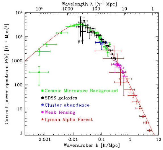
Figure 1: Linear matter power spectrum P(k) versus wavenumber extrapolated to z=0, from various measurements of cosmological structure. The best fit $\Lambda$CDM model is shown as a solid line. From [8].

At any epoch $t$ (or $a$ or $z)$ express the matter density in the universe in terms of a mean density and a local fluctuation:

$$\rho(\vec{x})=\bar{\rho}(1+\delta(\vec{x}))$$ (9)

where $\delta(\vec{x})$is the density contrast. Expand $\delta(\vec{x})$ in Fourier modes:

$$\delta(\vec{x})\equiv\frac{\rho(\vec{x})-\bar{\rho}}{\bar{\rho}}=\int{\delta(\vec{k})\exp(-i\vec{k}\cdot\vec{x})d^{3}}k.$$ (10)

The autocorrelation function of $\delta(\vec{x})$ defines the power spectrum through the relations

$$\left\langle{\delta(\vec{x})\delta(\vec{x})}\right\rangle=\int\limits_{0}^{\infty}{\frac{dk}{k}}\frac{k^{3}\left|{\delta^{2}(\vec{k})}\right|}{2\pi^{2}}=\int\limits_{0}^{\infty}{\frac{dk}{k}}\frac{k^{3}P(k)}{2\pi^{2}}=\int\limits_{0}^{\infty}{\frac{dk}{k}}\Delta^{2}(k)$$ (11)

where we have the definitions

$$P(k)\equiv\left|{\delta^{2}(\vec{k})}\right|,\mbox{ and }\Delta^{2}(k)\equiv\frac{k^{3}P(k)}{2\pi^{2}}.$$ (12)

The quantity $\Delta^{2}(k)$ is called the dimensionless power spectrum and is an important function in the theory of structure formation. $\Delta^{2}(k)$ measures the contribution of perturbations per unit logarithmic interval at wavenumber $k$ to the variance in the matter density fluctuations. The $\Lambda$CDM power spectrum asymptotes to $P(k)\sim k^{1}$ for small $k$, and $P(k)\sim k^{-3}$ for large $k$, with a peak a $k^{\star}\sim 2\times 10^{-2}$ h Mpc^-1 corresponding to $\lambda^{\star}\sim$350 h^-1 Mpc. $\Delta^{2}(k)$ is thus asymptotically flat at high $k$, but drops off as $k^{4}$ at small $k$. We therefore see that most of the variance in the cosmic density field in the universe at the present epoch is on scales $\lambda<\lambda^{\star}.$

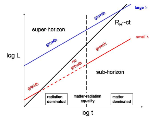
Figure 2: The tale of two fluctuations. A fluctuation which is superhorizon scale at matter-radiation equality grows always, while a fluctuation which enters the horizon during the radiation dominated era stops growing in amplitude until the matter dominated era begins.

What is the origin of the power spectrum shape? Here we review the basic ideas. Within the inflationary paradigm, it is believed that quantum mechanical (QM) fluctuations in the very early universe were stretched to macroscopic scales by the large expansion factor the universe underwent during inflation. Since QM fluctuations are random, the primordial density perturbations should be well described as a Gaussian random field. Measurements of the Gaussianity of the CMB anisotropies [11] have confirmed this. The primordial power spectrum is parameterized as a power law $P_{p}(k)\propto k^{n}$, with $n=1$ corresponding to scale-invariant spectrum proposed by Harrison and Zeldovich on the grounds that any other value would imply a preferred mass scale for fluctuations entering the Hubble horizon. Large angular scale CMB anisotropies measure the primordial power spectrum directly since they are superhorizon scale. Observations with the WMAP satellite are consistent with $n=1$.

To understand the origin of the spectrum, we need to understand how the amplitude of a fluctuation of fixed comoving wavelength $\lambda$ grows with time. Regardless of its wavelength, the fluctuation will pass through the Hubble horizon as illustrated in Fig. 2. This is because the Hubble radius grows linearly with time, while the proper wavelength a$\lambda$ grows more slowly with time. It is easy to show from Eq. 1 that in the radiation-dominated era, $a\sim t^{1/2}$, and in the matter-dominated era (prior to the onset of cosmic acceleration) $a\sim t^{2/3}$. Thus, inevitably, a fluctuation will transition from superhorizon to subhorizon scale. We are interested in how the amplitude of the fluctuation evolves during these two phases. Here we merely state the results of perturbation theory (e.g., Dodelson 2003, Ch. 7).

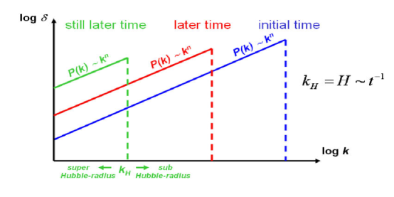
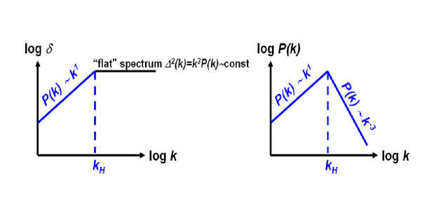
Figure 3: a) Evolution of the primordial power spectrum on superhorizon scales during the radiaton dominated era. b) Scale-free spectrum produces a constant contribution to the density variance per logarithmic wavenumber interval entering the Hubble horizon (no preferred scale) c) resulting matter power spectrum, super- and sub-horizon. Figures courtesy Rocky Kolb.

2.3 Growth of fluctuations in the linear regime

To calculate the growth of superhorizon scale fluctuations requires general relativistic perturbation theory, while subhorizon scale perturbations can be analyzed using a Newtonian Jeans analysis. We are interested in scalar density perturbations, because these couple to the stress tensor of the matter-radiation field. Vector perturbations (e.g., fluid turbulence) are not sourced by the stress-tensor, and decay rapidly due to cosmic expansion. Tensor perturbations are gravity waves, and also do not couple to the stress-tensor. A detailed analysis for the scalar perturbations yields the following results. In the radiation dominated era,

$$\begin{array}[]{l}\delta_{+}(t)=\delta_{+}(t_{i})(t/t_{i})\mbox{ superhorizon scales}\\ \delta_{+}(t)=constant\mbox{ ~{}~{}~{}subhorizon scales}\\ \end{array}$$

while in the matter dominated era,

$$\begin{array}[]{l}\delta_{+}(t)=\delta_{+}(t_{i})(t/t_{i})^{2/3}\mbox{ superhorizon scales}\\ \delta_{+}(t)=\delta_{+}(t_{i})(t/t_{i})^{2/3}\mbox{ subhorizon scales}\\ \end{array}$$

This is summarized in Fig. 2, where we consider two fluctuations of different comoving wavelengths, which we will call large and small. The large wavelength perturbation remains superhorizon through matter-radiation equality (MRE), and enters the horizon in the matter dominated era. Its amplitude will grow as $t$ in the radiation dominated era, and as $t^{2/3}$ in the matter dominated era. It will continue to grow as $t^{2/3}$ after it becomes subhorizon scale. The small wavelength perturbation becomes subhorizon before MRE. Its amplitude will grow as $t$ while it is superhorizon scale, remain constant while it is subhorizon during the radiation dominated era, and then grow as $t^{2/3}$ during the matter-dominated era.

Armed with these results, we can understand what is meant by a scale-free primordial power spectrum (the Harrison-Zeldovich power spectrum.) We are concerned with perturbation growth in the very early universe during the radiation dominated era. Superhorizon scale perturbation amplitudes grow as $t$, and then cease to grow after they have passed through the Hubble horizon. We can define a Hubble wave number $k_{H}\equiv 2\pi/R_{H}\propto t^{-1}.$ Fig. 3a shows the primordial power spectrum at three instants in time for k$<$k_H. We see that the fluctuation amplitude at k=k_H(t) depends on primordial power spectrum slope n. The scale-free spectrum is the value of n such that $\Delta^{2}(k_{H}(t))$=constant for k$>$k_H. A simple analysis shows that this implies n=1. Since $\Delta^{2}(k)\propto k^{3}P(k)$, we then have

$$\begin{array}[]{l}P(k)\propto k^{1},\mbox{ }k\leq k_{H}\\ P(k)\propto k^{-3},\mbox{ }k>k_{H}\\ \end{array}$$

In actuality, the power spectrum has a smooth maximum, rather than a peak as shown in Fig. 3c. This smoothing is caused by the different rates of growth before and after matter-radiation equality. The transition from radiation to matter-dominated is not instantaneous. Rather, the expansion rate of the universe changes smoothly through equality, as given by Eq. 1, and consequently so do the temporal growth rates. The position of the peak of the power spectrum is sensitive to the when the universe reached matter-radiation equality, and hence is a probe of $\Omega_{\gamma}/\Omega_{m}$.

Once a fluctuation becomes sub-horizon, dissipative processes modify the shape of the power spectrum in a scale-dependent way. Collisionless matter will freely stream out of overdense regions and smooth out the inhomogeneities. The faster the particle, the larger its free streaming length. Particles which are relativistic at MRE, such as light neutrinos, are called hot dark matter (HDM). They have a large free-streaming length, and consequently damp the power spectrum over a large range of k. Weakly Interacting Massive Particles (WIMPs) which are nonrelativistic at MRE, are called cold dark matter (CDM), and modify the power spectrum very little (Fig. 4). Baryons are tightly coupled to the radiation field by electron scattering prior to recombination. During rcombination, the photon mean-free path becomes large. As photons stream out of dense regions, they drag baryons along, erasing density fluctuations on small scales. This process is called Silk damping, and results in damped oscillations of the baryon-photon fluid once they become subhorizon scale. The magnitude of this effect is sensitive to the ratio of baryons to collisionless matter, as shown in Fig. 4.

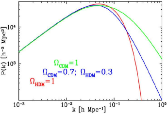
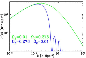
Figure 4: Effect of dissipative processes on the evolved power spectrum. Left: Effect of collisionless damping (free streaming) in the dark matter. Right: Effect of collisional damping (Silk damping) in the matter-radiation fluid. Figures courtesy Rocky Kolb.

3 Analytic models for nonlinear growth, virial scaling
relations, and halo statistics

Here we introduce a few concepts and analytic results from the theory of structure formation which underly the use of galaxy clusters as cosmological probes. These provide us with the vocabulary which pervades the literature on analytic and numerical models of galaxy cluster evolution. Material in this section has been derived from three primary sources: Padmanabhan (1993) [12] for the spherical top-hat model for nonlinear collapse, Dodelson (2003) [4] for Press-Schechter theory, and Bryan & Norman (1998) [13] for virial scaling relations.

3.1 Nonlinearity defined

In the linear regime, both super- and sub-horizon scale perturbations grow as $t^{2/3}$ in the matter-dominated era. This means that after recombination, the linear power spectrum retains its shape while its amplitude grows as $t^{4/3}$ before the onset of cosmic acceleration. When $\Delta^{2}(k)$ for a given k approaches unity linear theory no longer applies, and some other method must be used to determine the fluctuation’s growth. In general, numerical simulations are required to model the nonlinear phase of growth because in the nonlinear regime, the modes do not grow independently. Mode-mode coupling modifies both the shape and amplitude of the power spectrum over the range of wavenumbers that have gone nonlinear.

At any given time, there is a critical wavenumber which we shall call the nonlinear wavenumber k_nl which determines which portion of the spectrum has evolved into the nonlinear regime. Modes with k$<$k_nl are said to be linear, while those for which k$>$ k_nl are nonlinear. Conventionally, one defines the nonlinear wavenumber such that $\Delta(k_{nl},z)=1.$ From this one can derive a nonlinear mass scale $M_{nl}(z)=\frac{4\pi}{3}\bar{\rho}(z)\left({\frac{2\pi}{k_{nl}}}\right)^{3}$. A more useful and rigorous definition of the nonlinear mass scale comes from evaluating the amplitude of mass fluctuations within spheres or radius R at epoch z. The enclosed mass is $M=\frac{4\pi}{3}\bar{\rho}(z)R^{3}.$ The mean square mass fluctuations (variance) is

$$\left\langle{(\delta M/M)^{2}}\right\rangle\equiv\sigma^{2}(M)=\int{d^{3}kW_{T}^{2}(kR)P(k,z),}$$ (13)

where W is the Fourier transform of the top-hat window function

$$\begin{array}[]{l}\mbox{W(}{\rm{\bf x}}\mbox{)}=\left\{{{\begin{array}[]{*{20}c}{3/4\pi R^{3},\mbox{ }\left|{\rm{\bf x}}\right|<R\hfill}\\ {0,\mbox{ }\left|{\rm{\bf x}}\right|\geq R\hfill}\\ \end{array}}}\right.\\ \to W_{T}(kR)=3\left[{\sin(kR)/kR-\cos(kR)}\right]/(kR)^{2}.\\ \end{array}$$ (14)

If we approximate P(k) locally with a power-law $P(k,z)=D^{2}(z)k^{m}$, where D is the linear growth factor, then $\sigma^{2}(M)\propto D^{2}R^{-(3+m)}\propto D^{2}M^{-(3+m)/3}.$ From this we see that the RMS fluctuations are a decreasing function of M. At very small mass scales, m$\rightarrow-3$, and the fluctuations asymptote to a constant value. We now define the nonlinear mass scale by setting $\sigma$(M${}_{nl})$=1. We get that ([17])

$$M_{nl}(z)\propto D(z)^{6/(3+m)}\mbox{ (}\propto\mbox{(1}+\mbox{z)}^{\mbox{-6/(3}+\mbox{m)}}\mbox{ for EdS).}$$ (15)

For $m>-3$, the smallest mass scales become nonlinear first. This is the origin of hierarchical (“bottom-up”) structure formation.

3.2 Spherical Top-Hat Model

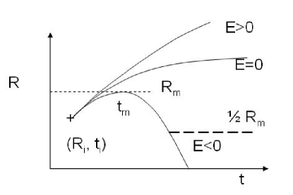
Figure 5: Evolution of a top-hat perturbation in an EdS universe. Depending on the E, the first integral of motion, the fluctuation collapses (E$<$0), continues to expand (E$>$0), or asymptotically reaches it maximum radius (E=0). Virialization occurs when the fluctuation has collapsed to half its turnaround radius.

We now ask what happens when a spherical volume of mass M and radius R exceeds the nonlinear mass scale. The simplest analytic model of the nonlinear evolution of a discrete perturbation is called the spherical top-hat model. In it, one imagines as spherical perturbation of radius $R$ and some constant overdensity $\bar{\delta}=3M/4\pi R^{3}$ in an Einstein-de Sitter (EdS) universe. By Birkhoff’s theorem the equation of motion for R is

$$\frac{d^{2}R}{dt^{2}}=-\frac{GM}{R^{2}}=-\frac{4\pi G}{3}\bar{\rho}(1+\bar{\delta})R$$ (16)

whereas the background universe expands according to Eq. 6

$$\frac{d^{2}a}{dt^{2}}=-\frac{4\pi G}{3}\bar{\rho}a.$$ (17)

Comparing these two equations, we see that the perturbation evolves like a universe of a different mean density, but with the same initial expansion rate. Integrating Eq. 16 once with respect to time gives us the first integral of motion:

$$\frac{1}{2}\left({\frac{dR}{dt}}\right)^{2}-\frac{GM}{R}=E,$$ (18)

where E is the total energy of the perturbation. If E$<$0, the perturbation is bound, and obeys

$$\frac{R}{R_{m}}=\frac{(1-cos\theta)}{2},~{}~{}~{}\frac{t}{t_{m}}=\frac{(\theta-sin\theta)}{\pi}$$ (19)

where $R_{m}$ and $t_{m}$ are the radius and time of “turnaround”. At turnaround (as $\theta\rightarrow\pi$), the fluctuation reaches its maximum proper radius (see Fig. 5). As $t\rightarrow 2t_{m},R\rightarrow 0$, and we say the fluctuation has collapsed.

A detailed analysis of the evolution of the top-hat perturbation is given in Padmanabhan (1993, Ch. 8) for general $\Omega_{m}$. Here we merely quote results for an EdS universe. The mean linear overdensity at turnaround; i.e., the value one would predict from the linear growth formula $\delta\sim t^{2/3}$, is 1.063. The actual overdensity at turnaround using the nonlinear model is 4.6. This illustrates that nonlinear effects set in well before the amplitude of a linear fluctuation reaches unity. As R$\rightarrow$0, the nonlinear overdensity becomes infinite. However, the linear overdensity at $t=2t_{m}$ is only 1.686. As the fluctuation collapses, other physical processes (pressure, shocks, violent relation) become important which establish a gravitationally bound object in virial equilibrium before infinite density is reached. Within the framework of the spherical top-hat model, we say virialization has occurred when the kinetic and gravitational energies satisfy virial equilibrium: $\left|U\right|=2K.$ It is easy to show from conservation of energy that this occurs when $R=R_{m}/2$; in other words, when the fluctuation has collapsed to half its turnaround radius. The nonlinear overdensity at virialization $\Delta_{c}$ is not infinite since the radius is finite. For an EdS universe, $\Delta_{c}=18\pi^{2}\approx 180$. Fitting formulae for non-EdS models are provided in the next section.

3.3 Virial Scaling Relations

The spherical top-hat model can be scaled to perturbations of arbitrary mass. Using virial equilibrium arguments, we can predict various physical properties of the virialized object. The ones that interest us most are those that relate to the observable properties of gas in galaxy clusters, such as temperature, X-ray luminosity, and SZ intensity change. Kaiser [14] first derived virial scaling relations for clusters in an EdS universe. Here we generalize the derivation to non-EdS models of interest. In order to compute these scaling laws, we must assume some model for the distribution of matter as a function of radius within the virialized object. A top-hat distribution with a density $\rho=\Delta_{c}\bar{\rho}(z)$ is not useful because it is not in mechanical equilibrium. More appropriate is the isothermal, self-gravitating, equilibrium sphere for the collisionless matter, whose density profile is related to the one-dimensional velocity dispersion [15]

$$\rho(r)=\frac{\sigma^{2}}{2\pi Gr^{2}}.$$ (20)

If we define the virial radius r_vir to be the radius of a spherical volume within which the mean density is $\Delta_{c}$ times the critical density at that redshift ($M=4\pi r_{vir}^{3}\rho_{crit}\Delta_{c}/3)$, then there is a relation between the virial mass M and $\sigma$:

$$\sigma=M^{1/3}[H^{2}(z)\Delta_{c}G^{2}/16]^{1/6}\approx 476f_{\sigma}\left({\frac{M}{10^{15}M_{\odot}}}\right)^{1/3}(h^{2}\Delta_{c}E^{2})^{1/6}\mbox{ km s}^{\mbox{-1}}.$$ (21)

Here we have introduced a normalization factor $f_{\sigma}$ which will be used to match the normailization from simulations. The redshift dependent Hubble parameter can be written as $H(z)=100hE(z)\mbox{ km s}^{-1}$ with the function $E^{2}(z)=\Omega_{m}(1+z)^{3}+\Omega_{k}(1+z)^{2}+\Omega_{\Lambda}$, where the $\Omega$’s have been previously defined.

The value of $\Delta_{c}$ is taken from the spherical top-hat model, and is 18$\pi^{2}$ for the critical EdS model, but has a dependence on cosmology through the parameter $\Omega(z)=\Omega_{m}(1+z)^{3}/E^{2}(z).$ Bryan and Norman (1998) provided fitting formulae for $\Delta_{c}$ for the critical for both open universe models and flat, lambda-dominated models

$$\Delta_{c}=18\pi^{2}+82x-39x^{2}\mbox{ for }\Omega_{k}=0,\mbox{ }\Delta_{c}=18\pi^{2}+60x-32x^{2}\mbox{ for }\Omega_{\Lambda}=0$$ (22)

where x=$\Omega$(z)-1.

If the distribution of the baryonic gas is also isothermal, we can define a ratio of the “temperature” of the collisionless material ($T_{\sigma}=\mu m_{p}\sigma^{2}/k)$ to the gas temperature:

$$\beta=\frac{\mu m_{p}\sigma^{2}}{kT}$$ (23)

Given equations (22) and (23), the relation between temperature and mass is then

$$kT=\frac{GM^{2/3}\mu m_{p}}{2\beta}\left[{\frac{H^{2}(z)\Delta_{c}}{2G}}\right]^{1/3}\approx 1.39f_{T}\left({\frac{M}{10^{15}M_{\odot}}}\right)^{2/3}(h^{2}\Delta_{c}E^{2})^{1/3}\mbox{ keV,}$$ (24)

where in the last expression we have added the normalization factor f_T and set $\beta$=1.

The scaling behavior for the object’s X-ray luminosity is easily computed by assuming bolometric bremsstrahlung emission and ignoring the temperature dependence of the Gaunt factor: $L_{bol}\propto\int{\rho^{2}}T^{1/2}dV\propto M_{b}\rho T^{1/2}.$ where M_b is the baryonic mass of the cluster. This is infinite for an isothermal density distribution, since $\rho$ is singular. Observationally and computationally, it is found that the baryon distribution rolls over to a constant density core at small radius. A procedure is described in Bryan and Norman (1998) which yields a finite luminosity:

$$L_{bol}=1.3\times 10^{45}\left({\frac{M}{10^{15}M_{\odot}}}\right)^{4/3}(h^{2}\Delta_{c}E^{2})^{7/6}\mbox{ }\left({\frac{\Omega_{b}}{\Omega_{m}}}\right)^{2}\mbox{ erg s}^{-1}.$$ (25)

Eliminating M in favor of T in Eq. 25 we get

$$L_{bol}=6.8\times 10^{44}\left({\frac{kT/f_{T}}{1.0\mbox{ keV}}}\right)^{2}(h^{2}\Delta_{c}E^{2})^{1/2}\mbox{ }\left({\frac{\Omega_{b}}{\Omega_{m}}}\right)^{2}\mbox{ erg s}^{-1}.$$ (26)

The scaling of the SZ “luminosity” is likewise easily computed. If we define L_SZ as the integrated SZ intensity change: $L_{SZ}=\int{dA\int{n_{e}\sigma_{T}}}\left({\frac{kT}{m_{e}c^{2}}}\right)dl\propto M_{b}T$, then

$$L_{SZ}=\frac{GM^{5/3}\sigma_{T}}{2\beta m_{e}c^{2}}\left[{\frac{H^{2}(z)\Delta_{c}}{2G}}\right]^{1/3}\left({\frac{\Omega_{b}}{\Omega_{m}}}\right).$$ (27)

We note that cosmology enters these relations only with the combination of parameters $h^{2}\Delta_{c}E^{2}$, which comes from the relation between the cluster’s mass and the mean density of the universe at redshift z. The redshift variation comes mostly from E(z), which is equal to (1+z)^3/2 for an EdS universe.

3.4 Statistics of hierarchical clustering: Press-Schechter theory

Now that we have a simple model for the nonlinear evolution of a spherical density fluctuation and its observable properties as a function of its virial mass, we would like to estimate the number of virialized objects of mass M as a function of redshift given the matter power spectrum. This is the key to using surveys of galaxy clusters as cosmological probes. While large scale numerical simulations can and have been used for this purpose (see below), we review a powerful analytic approach by Press and Schechter [16] which turns out to be remarkably close to numerical results. The basic idea is to imagine smoothing the cosmological density field at any epoch z on a scale R such that the mass scale of virialized objects of interest satisfies $M=\frac{4\pi}{3}\bar{\rho}(z)R^{3}.$ Because the density field (both smoothed and unsmoothed) is a Gaussian random field, the probability that the mean overdensity in spheres of radius R exceeds a critical overdensity $\delta_{c}$ is

$$p(R,z)=\frac{2}{\sqrt{2\pi}\sigma(R,z)}\int\limits_{\delta_{c}}^{\infty}{d\delta}\exp\left({-\frac{\delta^{2}}{2\sigma^{2}(R,z)}}\right)$$ (28)

where $\sigma(R,z)$ is the RMS density variation in spheres of radius R as discussed above. Press and Schechter suggested that this probability be identified with the fraction of particles which are part of a nonlinear lump with mass exceeding M if we take $\delta_{c}=1.686,$ the linear overdensity at virialization. This assumption has been tested against numerical simulations and found to be quite good [9]. The fraction of the volume collapsed into objects with mass between $M$ and $M+dM$ is given by $(dp/dM)dM$. Multiply this by the average number density of such objects $\rho_{m}/M$ to get the number density of collapsed objects between $M$ and $M+dM$:

$$dn(M,z)=-\frac{\bar{\rho}}{M}\frac{dp(M(R),z)}{dM}dM.$$ (29)

The minus sign appears here because p is a decreasing function of M. Carrying out the derivative using the fact that $dM/dR=3M/R,$ we get

$$\frac{dn(M,z)}{dM}=\sqrt{\frac{2}{\pi}}\frac{\bar{\rho}\delta_{c}}{3M^{2}\sigma}e^{-\delta_{c}^{2}/2\sigma^{2}}\left[{-\frac{d\ln\sigma}{d\ln R}}\right].$$ (30)

The term is square brackets is related to the logarithmic slope of the power spectrum, which on the mass scale of galaxy clusters is close to unity. Eq. 30 is called the halo mass function, and it has the form of a power law multiplied by an exponential. To make this more explicit, approximate the power spectrum on scales of interest as a power law as we have done above. Substituting the scaling relations for $\sigma$ in Eq. 30 one gets the result [17]

$$\frac{dn}{dM}=\left({\frac{2}{\pi}}\right)^{1/2}\frac{\bar{\rho}}{M^{2}}\left({1+\frac{m}{3}}\right)\left[{\frac{M}{M_{nl}(z)}}\right]^{\frac{m-3}{6}}\exp\left[{-\left({\frac{M}{M_{nl}(z)}}\right)^{\frac{3+m}{3}}/2}\right].$$ (31)

Here, $M_{nl}(z)$ is the nonlinear mass scale. To be more consistent with the spherical top-hat model, it satisfies the relation $\sigma(M_{nl},z)=\delta_{c}$; i.e., those fluctuations in the smoothed density field that have reached the linear overdensity for which the spherical top-hat model predicts virialization.

3.5 Application to galaxy clusters

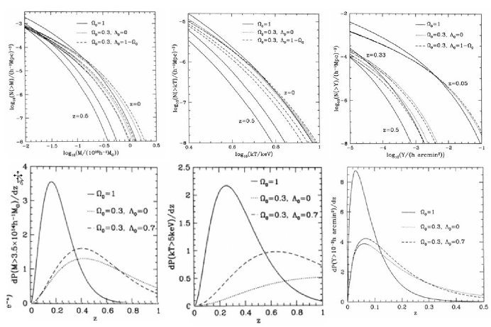
Figure 6: Top left to bottom right: a) Integrated cluster mass function for three cosmologies and two redshifts; b) like a), but for integrated temperature function; c) like a) but for integrated SZ cross section; d) redshift distribution of the integrated probability to find a cluster exceeding $M=3.5\times 10^{14}h^{-1}M_{\odot}$; e) redshift distribution of the integrated probability to find a cluster exceeding kT=5 keV; f) redshift distribution of the integrated probability to find a cluster exceeding Y=$10^{-3}$ h arcmin². From [18].

Galaxy clusters correspond to rare ($\sim$3$\sigma)$ peaks in the density field. Combining the halo mass function as prediced by the PS formalism with the scaling laws derived above, we can predict the evolution of the statistical properties of X-ray and SZ clusters of galaxies. Here we show a few results taken from Eke, Cole & Frenk (1996) [18]. Fig. 6a shows the evolution of the integrated mass function $n(>M)$ for several cosmologies and redshifts. One can see the power-law behavior at lower mass and the exponential cutoff at higher M. One sees strong redshift evolution of the number of massive clusters in the EdS model, but slower evolution on the open and lambda models. This is because of the saturated growth of structure in low density models. This makes number counts of massive clusters a sensitive test of the linear growth factor D(z), which depends on $\Omega_{m}$ and $\Omega_{\Lambda}$. Convolving the cluster population with the scaling relations for T(M) and Y(M), one gets distribution functions for n($>$T) and n($>$Y). Here $Y=L_{SZ}/d_{A}^{2}$ is the effective SZE cross section of a cluster, where $d_{A}$ is its angular diameter distance. These are shown in Figs. 6b and 6c. Another way to present the data is to convolve the mass function with the differential volume element as a function of redshift for the three models. Figs. 6d-f plot the redshift probability of detecting a cluster with M, T, and Y exceeding the fiducial values given in the figure caption. As one can see, the profiles are sharply peaked at low redshift for the EdS model, but substantially broader and peaking at higher redshift for the low density universe models. There is, however, rather little difference between the open and lambda-dominated models as far as the probability distributions for M and Y. Things are somewhat better for T, implying that some combination of X-ray and SZE measurements will be needed for precision cosmological parameter determinations.

4 Numerical simulations of gas in galaxy clusters

The central task is for a given cosmological model, calculate the formation and evolution of a population of clusters from which synthetic X-ray and SZ catalogs can be derived. These can be used to calibrate simpler analytic models, as well as to build synthetic surveys (mock catalogs) which can be used to assess instrumental effects and survey biases. One would like to directly simulate $n(M,z),n(L_{x},z),n(T,z),n(Y,z)$ from the governing equations for collisionless and collisional matter in an expanding universe. Clearly, the quality of these statistical predictions relies on the ability to adequately resolve the internal structure and thermodynamical evolution of the ICM.

In Norman (2003) [19] I provided a historical review of the progress that has been made in simulating the evolution of gas in galaxy clusters motivated by X-ray observations. Since X-ray emission and the SZE are both consequences of hot plasma bound in the cluster’s gravitational potential well, the requirements to faithfully simulate X-ray clusters and SZ clusters are essentially the same. Numerical progress can be characterized as a quest for higher resolution and essential baryonic physics. In this section I describe the technical challenges involved and the numerical methods that have been developed to overcome them. I then discuss the effects of assumed baryonic physics on ICM structure. Our point of reference is the non-radiative (so-called adiabatic) case, which has been the subject of an extensive code comparison [20]. I review the properties of adiabatic X-ray clusters, and show that they fail to reproduce observed cluster scaling laws. I then show results of numerical hydrodynamic simulations incorporating radiative cooling, star formation, and galaxy feedback and their associated scaling properties.

4.1 Dynamic range considerations

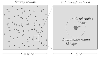
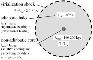
Figure 7: Left: A range of length scales of $\sim$250 separates the size of a reasonable survey volume and the virial radius of a rich cluster. Right: Simplified structure of the ICM in a massive cluster. A range of length scales of $\sim$20-30 separates the virial radius and the core radius.

Figure 7 illustrates the dynamic range difficulties encountered with simulating a statistical ensemble of galaxy clusters, while at the same time resolving their internal structure. Massive clusters are rare at any redshift, yet these are the ones most that are most sensitive to cosmology. From the cluster mass function (Fig. 6a), in order to get adequate statistics, one deduces that one must simulate a survey volume many hundreds of megaparsecs on a side (Fig. 7a). A massive cluster has a virial radius of $\sim$2 Mpc. It forms via the collapse of material within a comoving Lagrangian volume of $\sim$15 Mpc. However, tidal effects from a larger region (50-100 Mpc) are important on the dynamics of cluster formation. The internal structure of cluster’s ICM is shown in Fig. 7b. While clusters are not spherical, two important radii are generally used to characterize them: the virial radius, which is the approximate location of the virialization shock wave that thermalizes infalling gas to 10-100 million K, and the core radius, within which the baryon densities plateau and the highest X-ray emissions and SZ intensity changes are measured. A typical radius is $\sim$200 kpc. Within the core, radiative cooling and possibly other physical processes are important. Outside the core, cooling times are longer than the Hubble time, and the ICM gas is effectively adiabatic. If we wanted to achieve a spatial resolution of 1/10 of a core radius everywhere within the survey volume, we would need a spatial dynamic range of D=500 Mpc/20 kpc = 25,000. The mass dynamic range is more severe. If we want 1 million dark matter particles within the virial radius of a $10^{15}M_{\odot}$ cluster, then we would need $N_{particle}=M_{box}/M_{particle}=\Omega_{m}\rho_{crit}L^{3}/10^{9}\approx 10^{11}$ if they were uniformly distributed in the survey volume.

Two solutions to spatial dynamic range problem have been developed: tree codes for gridless N-body methods [21, 22] and adaptive mesh refinement (AMR) for Eulerian particle-mesh/hydrodynamic methods [23, 24, 25, 26]. Both methods increase the spatial resolution automatically in collapsing regions as described below. The solution to the mass dynamic range problem is the use of multi-mass initial conditions in which a hierarchy of particle masses is used, with many low mass particles concentrated in the region of interest. This approach has most recently used by Springel et al. (2000) [27], who simulated the formation of a galaxy cluster dark matter halo with $N=6.9\times 10^{6}$ dark matter particles, resolving the dark matter halos down to the mass scale of the Fornax dwarf spheroidal galaxy. The spatial dynamic range achieved in this simulation was $R=2\times 10^{5}$. Such dynamic ranges have not yet been achieved in galaxy cluster simulations with gas.

4.2 Simulating cluster formation

Simulations of cosmological structure formation are done in a cubic domain which is comoving with the expanding universe. Matter density and velocity fluctuations are initialized at the starting redshift chosen such that all modes in the volume are still in the linear regime. Once initialized, these fluctuations are then evolved to z=0 by solving the equations for collisionless N-body dynamics for cold dark matter, and the equations of ideal gas dynamics for the baryons in an expanding universe. Making the transformation from proper to comoving coordinates $\vec{r}=a(t)\vec{x}$, Newton’s laws for the collsionless dark matter particles become

$$\frac{d\vec{x}_{dm}}{dt}=\vec{\upsilon}_{dm},\mbox{ }\frac{d\vec{\upsilon}_{dm}}{dt}=-2\frac{\dot{a}}{a}\vec{\upsilon}_{dm}-\frac{1}{a^{2}}\nabla_{x}\phi$$ (32)

where $x$ and $v$ are the particle’s comoving position and peculiar velocity, respectively, and $\phi$ is the comoving gravitational potential that includes baryonic and dark matter contributions. The hydrodynamical equations for mass, momentum, and energy conservation in an expanding universe in comoving coordinates are ([28])

$$\begin{array}[]{l}\frac{\partial\rho_{b}}{\partial t}+\nabla\cdot(\rho_{b}\vec{\upsilon}_{b})+3\frac{\dot{a}}{a}\rho_{b}=0,\\ \frac{\partial(\rho_{b}\upsilon_{b,i})}{\partial t}+\nabla\cdot[(\rho_{b}\upsilon_{b,i})\vec{\upsilon}_{b}+5\frac{\dot{a}}{a}\rho_{b}\upsilon_{b,i}=-\frac{1}{a^{2}}\frac{\partial p}{\partial x_{i}}-\frac{\rho_{b}}{a^{2}}\frac{\partial\phi}{\partial x_{i}},\\ \frac{\partial e}{\partial t}+\nabla\cdot(e\vec{\upsilon}_{b})+p\nabla\cdot\vec{\upsilon}_{b}+3\frac{\dot{a}}{a}e=\Gamma-\Lambda,\\ \end{array}$$ (33)

where $\rho_{b},p$ and $e$, are the baryonic density, pressure and internal energy density defined in the proper reference frame, $\vec{\upsilon}_{b}$ is the comoving peculiar baryonic velocity, $a=1/(1+z)$ is the cosmological scale factor, and $\Gamma$ and $\Lambda$ are the microphysical heating and cooling rates. The baryonic and dark matter components are coupled through Poisson’s equation for the gravitational potential

$$\nabla^{2}\phi=4\pi Ga^{2}(\rho_{b}+\rho_{dm}-\bar{\rho}(z))$$ (34)

where $\bar{\rho}(z)=3H_{0}\Omega_{m}(0)/8\pi Ga^{3}$ is the proper background density of the universe.

The cosmological scale factor $a(t)$ is obtained by integrating the Friedmann equation (Eq. 4). To complete the specification of the problem we need the ideal gas equation of state $p=(\gamma-1)e$, and the gas heating and cooling rates. When simulating the ICM, the simplest approximation is to assume $\Gamma$ and $\Lambda=0$; i.e., no heating or cooling of the gas other than by adiabatic processes and shock heating. Such simulations are referred to as adiabatic (despite entropy-creating shock waves), and are a reasonable first approximation to real clusters because except in the cores of clusters, the radiative cooling time is longer than a Hubble time, and gravitational heating is much larger than sources of astrophysical heating. However, as discussed in the paper by Cavaliere in this volume, there is strong evidence that the gas in cores of clusters has evolved non-adiabatically. This is revealed by the entropy profiles observed in clusters [29] which deviate substantially from adiabatic predictions. In the simulations presented below, we consider radiative cooling due to thermal bremsstrahlung, and mechanical heating due to galaxy feedback, details of which are described below.

4.3 Numerical methods overview

A great deal of literature exists on the gravitational clustering of CDM using N-body simulations. A variety of methods have been employed including the fast grid-based methods particle-mesh (PM), and particle-particle+particle-mesh (P³M) [30], spatially adaptive methods such as adaptive P³M [31], adaptive mesh refinement [24], tree codes [32, 33], and hybrid methods such as TreePM [34]. Because of the large dynamic range required, spatially adaptive methods are favored, with Tree and TreePM methods the most widely used today. When gas dynamics is included, only certain combinations of hydrodynamics algorithms and collisionless N-body algorithms are “natural”. Dynamic range considerations have led to two principal approaches: P³MSPH and TreeSPH, which marries a P³M or tree code for the dark matter with the Lagrangian smoothed-particle-hydrodynamics (SPH) method [35, 21, 22], and adaptive mesh refinement (AMR), which marries PM with Eulerian finite-volume gas dynamics schemes on a spatially adaptive mesh [23, 26, 25, 36]. Pioneering hydrodynamic simulations using non-adaptive Eulerian grids [37, 38, 13] yielded some important insights about cluster formation and statistics, but generally have inadequate resolution to resolve their internal structure in large survey volumes. In the following we concentrate on our latest results using the AMR code Enzo [26]. The reader is also referred to the paper by Borgani et al. [39] which presents recent, high-resolution results from a large TreeSPH simulation.

Enzo is a grid-based hybrid code (hydro + N-body) which uses the block-structured AMR algorithm of Berger & Collela [40] to improve spatial resolution in regions of large gradients, such as in gravitationally collapsing objects. The method is attractive for cosmological applications because it: (1) is spatially- and time-adaptive, (2) uses accurate and well-tested grid-based methods for solving the hydrodynamics equations, and (3) can be well optimized and parallelized. The central idea behind AMR is to solve the evolution equations on a grid, adding finer meshes in regions that require enhanced resolution. Mesh refinement can be continued to an arbitrary level, based on criteria involving any combination of overdensity (dark matter and/or baryon), Jeans length, cooling time, etc., enabling us to tailor the adaptivity to the problem of interest. The code solves the following physics models: collisionless dark matter and star particles, using the particle-mesh N-body technique [41]; gravity, using FFTs on the root grid and multigrid relaxation on the subgrids; cosmic expansion; gas dynamics, using the piecewise parabolic method (PPM)[42]; multispecies nonequilibrium ionization and H₂ chemistry, using backward Euler time differencing [28]; radiative heating and cooling, using subcycled forward Euler time differencing [43]; and a parameterized star formation/ feedback recipe [44]. At the present time, magnetic fields and radiation transport are being installed. Enzo is publicly available at http://cosmos.ucsd.edu/enzo.

4.4 Structure of nonradiative clusters: the Santa Barbara test cluster

In Frenk et al. [20] 12 groups compared the results of a variety of hydrodynamic cosmological algorithms on a standard test problem. The test problem, called the Santa Barbara cluster, was to simulate the formation of a Coma-like cluster in a standard CDM cosmology ($\Omega_{m}=1$) assuming the gas is nonradiative. Groups were provided with uniform initial conditions and were asked to carry out a “best effort” computation, and analyze their results at z=0.5 and z=0 for a set of specified outputs. These outputs included global integrated quantities, radial profiles, and column-integrated images. The simulations varied substantially in their spatial and mass resolution owing to algorithmic and hardware limitations. Nonetheless, the comparisons brought out which predicted quantities were robust, and which were not yet converged. In Fig. 8 we show a few figures from Frenk et al. (1999) which highlight areas of agreement (top row) and disagreement (bottom row).

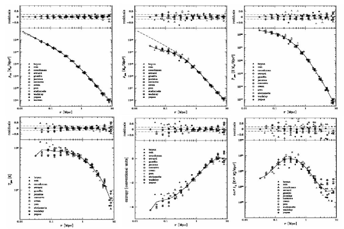
Figure 8: The Santa Barbara test cluster. Top row, left to right: profiles of dark matter density, gas density, and gas pressure. Bottom row, left to right: profiles of gas temperature, gas entropy, and X-ray emissivity. Different symbols correspond to different code results. From [20].

The top row shows profile of dark matter density, baryon density, and pressure for the different codes. All are in quite good agreement for the mechanical structure of the cluster. The dark matter profile is well described by an NFW profile which has a central cusp [45]. The baryon density profiles show more dispersion, but all codes agree that the profile flattens at small radius, as observed. All codes agree extremely well on the gas pressure profile, which is not surprising, since mechanical equilibrium is easy to achieve for all methods even with limited resolution. This bodes well for the interpretation of SZE observations of clusters, since the Compton y parameter is proportional to the projected pressure distribution. In section 5 we show results from a statistical ensemble of clusters which bear this out.

The bottom row shows the thermodynamic structure of the cluster, as well as the profile of X-ray emissivity. The temperature profiles show a lot of scatter within about one-third the virial radius (=2.7 Mpc). Systematically, the SPH codes produce nearly isothermal cores, while the grid codes produce temperature profiles which continue to rise as r$\rightarrow$0. The origin of this discrepancy has not been resolved, but improved SPH formulations come closer to reproducing the AMR results [51]. This discrepancy is reflected in the entropy profiles. Again, agreement is good in the outer two-thirds of the cluster, but the profiles show a lot of dispersion in the inner one third. Discounting the codes with inadequate resolution, one finds the SPH codes produce an entropy profile which continues to fall as r$\rightarrow$0, while the grid codes show an entropy core, which is more consistent with observations [29]. The dispersion in the density and temperature profiles are amplified in the X-ray emissivity profile, since $\varepsilon_{x}\propto\rho_{b}^{2}T^{1/2}$. The different codes agree on the integrated X-ray luminosity of the cluster only to within a factor of 2. This is primarily because the density profile is quite sensitive to resolution in the core; any underestimate in the core density due to inadequate resolution is amplified by the density squared dependence of the emissivity. This suggests that quite high resolution is needed, as well as a good grasp on non-adiabatic processes operating in cluster cores, before simulations will be able to accurately predict X-ray luminosities.

4.5 A numerical sample of adiabatic clusters: Universal Temperature Profile

Three questions one can ask about the Santa Barbara cluster results are: 1) is the cluster statistically representative, 2) do the results change substantially for a $\Lambda$CDM cosmology (the SB cluster assumed an EdS cosmology), and 3) what is the effect of additional baryonic physics on cluster structure? We address these questions here by summarizing results of Enzo simulations of the ICM in a sample of clusters in a concordance $\Lambda$CDM model drawn from a survey volume 256h^-1 Mpc on a side. Multimass initial conditions and AMR are used to achieve high spatial and mass resolution within the clusters. More details can be found in [47, 48, 46, 49].

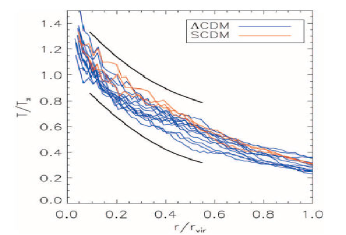
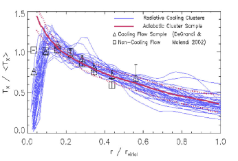
Figure 9: Left: Temperature profiles from a sample of adiabatic cluster simulations (from Loken et al. 2002). Black curves bound the 1s confidence band from Markevitch et al. (1998). Right: Effect of radiative cooling on temperature profiles, compared with adiabatic sample average (red line) and observational data for cooling flow clusters (triangles) and non-cooling flow clusters (squares).

Fig. 9 shows spherically averaged temperature profiles for 13(3) $\Lambda$CDM(SCDM) simulated clusters at z=0 analyzed by Loken et al. (2002) [47]. These were chosen from a total sample of 22(10) clusters because their 2D projected temperature maps were symmetric; the rejected non-symmetric clusters were in various states of merging. The smooth black curves bound the 1$\sigma$ confidence band from Markevitch et al. (1998)[62] who analyzed temperature profiles from a sample of 17 symmetric X-ray clusters observed with ASCA. When temperature is normalized by the integrated emission-weighted temperature and the radius by the virial radius, both the observed data and the simulated data collapse to a narrow band, suggesting a universal temperature profile (UTP) outside the core region. The fit to the numerical data is $T\propto(1+r/\alpha)^{-\delta}$, with $\alpha\sim$r_vir/1.5 and $\delta\sim$1.6. The $\Lambda$CDM clusters and SCDM clusters exhibit the same profile, with a suggestion of a slightly higher normalization for clusters in the critically closed model. The fit is in good agreement with observations over the range 0.2$<$r/r${}_{vir}<$0.5, but diverges at small radius where the effects of non-adiabatic processes appear to be at play [63]. The reality of the UTP was somewhat controversial when early results from Newton/XMM were showing large isothermal cores. However, the latest Chandra observations of 13 nearby, relaxed clusters have shown that the UTP provides an excellent description for temperature profiles outside $r\sim 0.15r_{vir}$ [50]. Subsequent numerical studies by Ascasibar et al. [51] and Borgani et al. [39] using SPH have found agreement with the AMR results of Loken et al. The general agreement of numerical and observational results suggests that the declining temperature profile is a natural consequence of gravitational heating of the ICM during the process of cluster formation.

4.6 Effect of additional physics

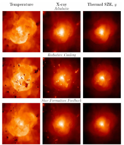
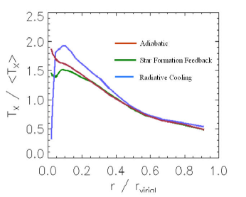
Figure 10: Left: Columns show X-ray surface brightness, projected temperature, and Compton y-parameter for a $M=2\times 10^{15}M_{\odot}$ cluster assuming different baryonic physics. Field of view is 5 h^-1 Mpc. Right: Corresponding spherically averaged radial temperature profiles.

Within r=0.15 r_vir, Vikhlinin et al. [50] found large variation in temperature profiles, but in all cases the gas is cooler than the cluster mean. This suggests that radiative cooling is important in cluster cores, and possibly other effects as well. It has been long known that $\sim 60$ percent of nearby, luminous X-ray clusters have central X-ray excesses, which has been interpreted as evidence for the presence of a cluster-wide cooling flows [64]. More recently, Ponman et al. [29] have used X-ray observations to deduce the entropy profiles in galaxy groups and clusters. They find an entropy floor in the cores of clusters indicative of extra, non-gravitational heating, which they suggest is feedback from galaxy formation. It is easy to imagine cooling and heating both may be important to the thermodynamic evolution of ICM gas.

To explore the effects of additional physics on the ICM, we recomputed the entire sample of clusters changing the assumed baryonic physics, keeping initial conditions the same. Three additional samples of about 100 clusters each were simulated: The “radiative cooling” sample assumes no additional heating, but gas is allowed to cool due to X-ray line and bremsstrahlung emission in a 0.3 solar metallicity plasma. The “star formation” sample uses the same cooling, but additionally cold gas is turned into collisionless star particles at a rate $\dot{\rho}_{SF}=\varepsilon_{sf}\frac{\rho_{b}}{\max(\tau_{cool},\tau_{dyn})}$ , where $\varepsilon_{sf}$ is the star formation efficiency factor $\sim$0.1, and $\tau_{cool}$ and $\tau_{dyn}$ are the local cooling time and freefall time, respectively. This locks up cold baryons in a non-X-ray emitting component, which has been shown to have an important effect of the entropy profile of the remaining hot gas [56, 57]. Finally, we have the “star formation feedback” sample, which is similar to the previous sample, except that newly formed stars return a fraction of their rest mass energy as thermal and mechanical energy. The source of this energy is high velocity winds and supernova energy from massive stars. In Enzo, we implement this as thermal heating in every cell forming stars: $\Gamma_{sf}=\varepsilon_{SN}\dot{\rho}_{SF}c^{2}$. The feedback parameter depends on the assumed stellar IMF the explosion energy of individual supernovae. It is estimated to be in the range $10^{-6}\leq\varepsilon_{SN}\leq 10^{-5}$ [44]. We treat it as a free parameter.

Fig. 10 shows synthetic maps of X-ray surface brightness, temperature, and Compton y-parameter for a $M=2\times 10^{15}M_{\odot}$ cluster at z=0 for the three cases indicated. The “star formation” case is omitted because the images are very similar to the “star formation feedback” case (see reference [46].) The adiabatic cluster shows that the X-ray emission is highly concentrated to the cluster core. The projected temperature distribution shows a lot of substructure, which is true for the adiabatic sample as a whole [47]. A complex virialization shock is toward the edge of the frame. The y-parameter is smooth, relatively symmetric, and centrally concentrated. The inclusion of radiative cooling has a strong effect on the temperature and X-ray maps, but relatively little effect on the SZE map. The significance of this is discussed in Section 5. In simulations with radiative cooling only, dense gas in merging subclusters cools to 10⁴ K and is brought into the cluster core intact [48]. These cold lumps are visible as dark spots in the temperature map. They appear as X-ray bright features. The inclusion of star formation and energy feedback erases these cold lumps, producing maps in all three quantities that resemble slightly smoothed versions of the adiabatic maps. However, an analysis of the radial temperature profiles (Fig. 10) reveal important differences in the cluster core. The temperature continues to rise toward smaller radii in the adiabatic case, while it plummets to $\sim$10⁴ K for the radiative cooling case. While the temperature profile looks qualitatively similar to observations of so-called cooling flow clusters, our central temperature is too low and the X-ray brightness too high. The star formation feedback case converts the cool gas into stars, and yields a temperature profile which follows the UTP at $r\geq 0.15r_{vir}$, but flattens out at smaller radii. This is consistent with the high resolution Chandra observations of Vikhlinin et al. [50].

5 Comparisons and predictions for X-ray and SZE surveys

In this section we shall compare the results of numerical hydrodynamical simulations with the analytic scaling laws derived in section 3, and compare with observational data. We will see that the X-ray temperature and the integrated SZE is a robust indicator of cluster mass with relatively little bias, while the X-ray luminosity is not because we cannot reliably simulate the X-ray emission from clusters.

5.1 Analytic and numerical comparisons

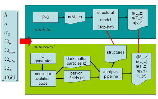
Figure 11: Comparing analytic and numerical predictions for cluster statistics.

We first ask the question how well do the simple analytic model estimates of cluster statistics agree with the results of numerical hydrodynamic simulations. This question was addressed by Bryan & Norman 1998 [13]. Fig. 11 illustrates how the comparisons are made. For a given cosmological model Press-Schechter theory is used to calculate the halo mass function versus redshift (top rectangle). The observable quantities $n(T,z),N(L_{x},z),n(Y,z)$ are then computed using the scaling relations presented in Section 3 for $L_{x},T$ and $Y$ as a function of mass. Somewhat more work is involved deriving these results from numerical simulation (bottom rectangle). Initial conditions for the chosen cosmology are generated which specify dark matter and baryonic perturbations at the starting redshift. These perturbations are evolved use in the methods described in section 4 to z=0. The particle and baryonic distributions are output at specified redshifts for analysis. Virialized objects are located using a group-finding algorithm on the dark matter particles list. Two popular techniques are friends-of-friends [52] and HOP [53]. In the friends-of-friends algorithm, two particles are part of the same group if their separation is less than some chosen value; chains of pairs then define groups. In the HOP algorithm, an estimate of the local density is associated with every particle. Each particle is linked to its densest neighbor and on to that particle’s densest neighbor until one reaches the particle which is its own densest neighbor. All particles that are traced to the same such particle define the group. Once groups are found, centers of masses for each group are computed. With these centers determined, spherically averaged profiles of dark matter density, baryon density, temperature, etc. are computed by binning the 3D data into spherical shells. For each halo, the virial radius is determined by find the shell inside of which the mean total density (dark matter + baryons) equals the critical overdensity $\Delta_{c}$ (Section 3). Virial mass, X-ray luminosity, and emission weighted temperature are computed by numerical integration over the radial profiles of total density, X-ray emissivity, etc. With these quantities evaluated for each cluster in the sample, distribution functions are then computed.

5.2 Cluster temperatures

One of the most robust predictions of numerical simulations is the mass-temperature relation. Fig. 12a shows a comparison between analytic scaling relations and simulations for two cosmological models at three epochs. The simulations were carried out on fixed Eulerian grids of size 270³ and 512³ assuming the clusters are non-radiative. Good agreement is seen with a slight offset in normalization. Fitting Eq. 24 to the data yields $f_{T}\approx 0.8.$ That the simulations reproduce the analytic scaling relations despite limited numerical resolution is a consequence of energy conservation, which is maintained to high accuracy by the numerical hydrodynamic method employed. Note that a cluster of a given mass is cooler at lower redshifts.

Fig. 12b shows the temperature distribution function as predicted by simulations (histograms) and Press-Schechter theory (curves) for a critically closed model (SCDM) and a low density model (OCDM). Generally, agreement is good. Simulations underpredict the number of low temperature clusters due to resolution effects. The high temperature clusters are rare, and thus not many are found in our small box. Despite these numerical limitations, one sees that the number of hot clusters evolves rapidly in the flat universe but evolves very little in the open universe.

Fig. 13a shows the predictions of simulations compared with the observational data of Henry & Arnaud (1991)[54]. The SCDM model is ruled out with high confidence, while the CHDM and OCDM models are marginally consistent with data. Eke, Cole & Frenk (1996) [18] showed that with a suitable adjustment of $\sigma_{8}$, a critically closed, open, and $\Lambda$-dominated models could all reproduce the observations (Fig. 13b). This illustrates what is known as the $\Omega_{0}-\sigma_{8}$ degeneracy in cluster abundances [55]. The redshift evolution of cluster abundances can in principle break this degeneracy, however this requires large samples of high redhift clusters with accurately measured temperatures. So far, the samples are small. Temperatures are more difficult to measure than X-ray luminosities. Nonetheless, available data shows mild evolution of the X-ray temperature function, consistent with a low density universe [3].

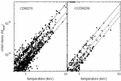
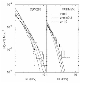
Figure 12: Left: M-T scaling in a flat $\Omega_{m}$=1 universe (left) and an open $\Omega_{m}$=0.34 universe (right) for z=0, 0.5, and 1 (top to bottom). Symbols are measured values hydrodynamic simulations. Lines are the scaling relations from Eq. 24. with f_T=0.8 (from [13]). Right: Evolution of cumulative temperature distribution function for the two models shown in Fig 13 as predicted by theory (curves) and hydrodynamic simulations (histograms). The number of hot clusters evolves rapidly in the flat universe but evolves very little in the open universe.

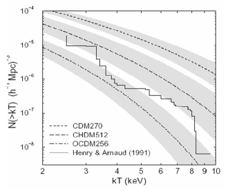
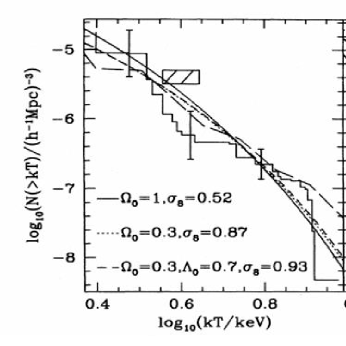
Figure 13: Left: Comparison of z=0 cluster temperature function from Henry & Arnaud (1991) with hydrodynamic simulations. SCDM model ($\Omega_{0}$=1, $\sigma_{8}$=1.05) is ruled out with high confidence, OCDM model ($\Omega_{0}$=0.34, $\sigma_{8}$=0.75) is marginally consistent with data. (from Bryan & Norman 1998). Right: Figure 18. Illustration of the $\Omega_{0}-\sigma_{8}$ degeneracy. Good agreement with data is found for flat, open, and $\Lambda$-dominated cosmological models with a suitable adjustment of $\sigma_{8}$. From [18].

5.3 Cluster X-ray luminosities

The most easily measured property of an X-ray cluster is its luminosity. However, as we shall see, this is the most difficult quantity to predict using numerical simulations. This is because the integrated X-ray luminosity of a cluster is dominated by emission from the core region, which is challenging to resolve numerically, and it is affected by heating and cooling processes which are as yet not well understood. The advent of multiscale numerical simulation techniques has ameliorated the numerical resolution difficulties. As one can see from Fig. 8f, the X-ray emissivity peaks at about $0.1r_{vir}$ for the adiabatic Santa Barbara cluster. SPH and AMR simulations can now resolve this scale with ten resolution elements or more in large cosmological volumes. Fig. 14 shows the $L_{x}-M$ and $L_{x}-T$ scaling relation derived from our large sample of adiabatic galaxy clusters simulated using AMR in a $\Lambda$CDM universe. The numerical clusters are in good agreement with the analytic virial scaling relations $L_{x}\propto M^{4/3}$ and $L_{x}\propto T^{2}$ without resort to resolution corrections (cf. Bryan & Norman 1998). However, the adiabatic models are in conflict with the observed scaling relation, which are $L_{x}\propto M^{1.8}$ and $L_{x}\propto T^{3}$ for $T>2$ keV [3].

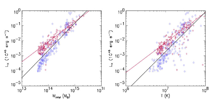
Figure 14: High resolution AMR simulations of adiabatic clusters (red crosses) agree with analytic scaling predictions (red lines), but disagree with observations (black lines). Addition of radiative cooling (blue diamonds) improves agreement, but produces too many clusters with cool cores. Figures courtesy P. Motl.

The disagreement between the predictions of adiabatic simulations and observations can be taken as strong evidence of the importance of non-adiabatic processes in the cores of galaxy clusters. The effect of radiative cooling is shown by the open diamonds in Fig. 14. Although the $L_{x}-M$ and $L_{x}-T$ scaling steepens in the direction of observations, we view these models as unrealistic since every cluster in the sample has too much cold gas in the core, contrary to observations. The scaling relations for the “star formation” and “star formation feedback” samples are show in Fig. 15a. The conversion of cool gas into stars produces clusters whose temperature and X-ray surface brightness profiles are in better agreement with observations, and steepens the $L_{x}-T$ relation somewhat relative the to adiabatic clusters. The inclusion of supernova heating has a rather minor effect when compared to the magnitude of the change including star formation. This is best illustrated in Fig. 15b, which shows the scatter of central entropy versus central temperature for the adiabatic, star formation, and star formation feedback cluster samples. An analysis of a sample of clusters by Ponman et al. (1999) [29] revealed the existence of an “entropy floor”. This feature has been interpreted as evidence of galaxy formation feedback which increases gas entropy. The same data has been explained as the result of radiative cooling [56, 57] which locks up low entropy gas in stars where it does not contribute to X-ray emission. The magnitude of the entropy floor strongly suggests the heating explanation. The failure of star formation feedback simuations to exhibit the entropy floor may be due to limited mass resolution. The galaxy mass function is not well sampled is these simulations; indeed, only the central dominant galaxy and one or two of the most massive galaxies are present in these simulations. Perhaps higher resolution simuations will improve agreement. AGN heating is another source of energy input that may be important, especially in the cores of clusters [58]. Numerical simulations incorporating these effects are in their infancy, and certainly not at the stage where large ensembles can be simulated for statistical analysis.

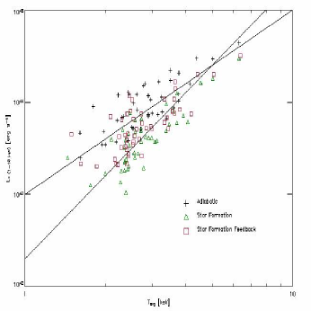
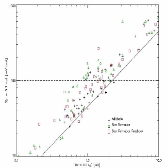
Figure 15: Left: Effect of baryonic physics on the L-T relation for three AMR cluster samples: adiabatic (crosses), star formation (triangles), and star formation feedback (squares). Right: Central entropy versus central temperature for the cluster samples in Fig 12. The dashed line is the observed “entropy floor”. Figures courtesy P. Motl.

5.4 Prospects for SZE cluster surveys

The sensitivity of X-ray luminosity to numerical resolution and baryonic processes motivates us to look for other more robust indicators of a cluster’s mass. Temperature is such an indicator, however this is more difficult to measure than X-ray luminosity even at low redshifts. At high redshifts the task becomes even more difficult because of the severe $(1+z)^{-4}$ surface brightness dimming of the X-ray flux. In this section we explore the thermal SZE effect as a mass indicator based on our four catalogs of simulated galaxy clusters. Based on these models, we find that the integrated SZE $y_{500}$ is a less biased indicator of cluster mass than either the X-ray luminosity or temperature, and shows far less scatter than the central value of the SZE intensity change $y_{0}$. More details can be found in references [46, 49]

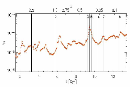
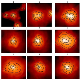
Figure 16: Left: The “lightcurve” for the central value of the Compton parameter, $y_{0}$, obtained from tracking one particular halo from a redshift of 4 to the present epoch. Major mergers can boost $y_{0}$ by a factor of 10. Right: Projected y parameter distribution of cluster at the epochs marked by vertical lines in the lightcurve. Figures courtesy P. Motl.

As has been discussed elsewhere in this volume (Rephaeli, Birkinshaw), the thermal SZE is an attractive cosmological probe because it is redshift independent. The strength of the SZE is proportional to the Compton parameter, y, which for non-relativistic electrons is essentially the integral of the gas pressure through the cluster

$$y=\int{\frac{k_{B}T}{m_{e}c^{2}}}\sigma_{T}n_{e}d\ell\propto\int{nTd\ell.}$$ (35)

The central value of the Compton y parameter we refer to as $y_{0}$. We define the integrated SZE $y_{500}$ as the area integral of the y parameter out to $r_{500}$, the radius inside of which the mean density is 500 times the critical density:

$$y_{500}=2\pi\int\limits_{0}^{r_{500}}{y(r)rdr.}$$ (36)

The detectability of a cluster is given by its SZ cross section (Section 3), which is essentially $y_{500}/d_{A}^{2}\propto(1+z)^{-2}$. This is far more favorable redshift dependence than X-rays provide.

Fig. 16a shows the redshift evolution of $y_{0}$ for the most massive cluster in our sample. As can be seen, $y_{0}$ exhibits a secular increase as the cluster potential deepens, but is boosted by up to a factor of $\sim$20(2) during major(minor) merger events. The duration of these events is of order the dynamical time $\sim$1-2 Gyr. The effect of mergers induces considerable scatter into scaling between $y_{0}$ and the enclosed mass $M_{500}$ in our sample of clusters at z=0 (Fig. 17a). By contrast, $y_{500}$ shows a much tighter correlation (Fig. 17b). The reason for this is illustrated in the lower two panels of Fig. 17 where we plot the central value of the gas pressure $p_{0}$ and the volume averaged pressure $p_{500}=\frac{3}{4\pi r_{500}^{3}}\int\limits_{0}^{r_{500}}{p(\vec{x})d^{3}\vec{x}}$. The central pressure exhibits large scatter due to the presence of shock waves induced by mergers. However, the volume averaged pressure exhibits relatively little scatter. This is a consequence of virial equilibrium and tells us that the clusters are approximately in equilibrium within $r_{500}$.

Fitting the data to a power law of the form

$$y_{500}=A\left[{\frac{M_{500}}{10^{14}M_{\odot}}}\right]^{\alpha}$$ (37)

for each of our 4 catalogs, we find $\alpha\sim 1.6,\sigma_{\alpha}\sim 0.025$ for the adiabatic, star formation, and star formation feedback samples, and $\alpha\sim 1.7,\sigma_{\alpha}\sim 0.03$ for the radiative cooling sample. The scaling exponent is consistent with the findings of da Silva et al (2004) [59]. Ignoring the radiative cooling only runs as unrealistic, we find that the scaling is relatively insensitive to baryonic physics. This is both reassuring and understandable in that regardless of the thermodynamics of the gas, hydrostatic equilibrium is maintained to a good approximation. By looking back through our catalogs in redshift, we find that the coefficient A is independent of redshift.

Figure 17: Upper: The scaling relations between $y_{0}$ and $y_{500}$ and the total cluster mass within the same radius at z=0 for the star formation with feedback cluster sample. Two randomly chosen, orthogonal projections for each cluster are plotted as individual points and the catalog contains $\sim 100$ clusters at this epoch in the mass range $1\times 10^{14}M_{\odot}\leq M_{200}\leq 2\times 10^{15}M_{\odot}$. The best fit relations are plotted as solid lines. Lower: Central pressure and pressure integrated inside sphere of radius $r_{500}$ plotted against cluster total mass. From [46].

5.5 Cluster mass estimates compared

To assess the systematic biases and relative scatter of various means of estimating cluster masses from X-ray and SZE data, we “observed” our four clusters samples and analyzed the resulting synthetic images in the same way as observations. Our goal was to find both the best cluster mass estimator and best method of analysis. These were defined as the combination which produce the least bias and smallest scatter between inferred cluster mass and actual (simulated) mass. Here we merely summarize our findings; for details the reader is referred to [49].

Cluster masses can be obtained from X-ray and thermal SZE observations in several ways. The most widely used is the isothermal beta model, wherein it is assumed the electron number density is spherically symmetric and follows

$$n_{e}(r)=n_{e0}\left[{1+\left({\frac{r}{r_{c}}}\right)^{2}}\right]^{-3\beta/2},$$ (38)

where $n_{e0}$ is the central electron density. Approximating the gas as isothermal with average temperature $\langle T\rangle$ within the fitting radius, then the X-ray surface brightness is

$$S_{X}(r)=S_{X0}\left[{1+\left({\frac{r}{r_{c}}}\right)^{2}}\right]^{\frac{1}{2}-3\beta}$$ (39)

where $S_{X0}\propto n_{e0}^{2}\left\langle T\right\rangle^{\frac{1}{2}}$. Similarly for the SZE, a beta model density distribution results in a projected radial distribution for the Compton y parameter

$$y(r)=y_{0}\left[{1+\left({\frac{r}{r_{c}}}\right)^{2}}\right]^{\frac{1}{2}-\frac{3\beta}{2}}$$ (40)

where $y_{0}\propto n_{e0}\left\langle T\right\rangle.$

By fitting the observed profiles of $S_{x}(r)$ and $y(r)$ one obtains $\beta$ and $r_{c}$, the core radius. With $\left\langle T\right\rangle$ measured observationally, $n_{e0}$ can then be calculated. One then integrates Eq. 38 to find the gas mass within the fitting radius $r_{<}$. The cluster dynamical mass is then $M_{dyn}(r_{<})=M_{gas}(r_{<})/f_{b}(r_{<}),$ where $f_{b}$ is the baryon fraction which may in general be different from the cosmic mean $\Omega_{m}/\Omega_{b}$ depending upon the radius. Henceforth we will refer to mass estimates made in this way as X-ray-ISO and SZE-ISO.

Recently is has been shown both in simulations (Loken et al. 2002, Section 4) and in X-ray observations (Vikhlinin et al. 2005) that clusters are not isothemal at large radii, but follow a universal temperature profile (UTP)

$$T(r)=\left\langle T\right\rangle_{500}\left[{1+\left({\frac{r}{\alpha r_{500}}}\right)^{2}}\right]^{-\delta}$$ (41)

where $\langle T_{500}\rangle$ is the average temperature inside $r_{500}$, and $\alpha$ and $\delta$ are fitting parameters determined from a large sample of clusters. Improved mass estimates can be obtained by geometric deprojection of the X-ray and SZE profiles if one knows the temperature of each radial shell. This is provided by the UTP. For example, the X-ray surface brightness can be deprojected to yield the X-ray emissivity in each spherical shell (e.g., [60]). Knowing the temperature profile, once can obtain the mass in each shell. A similar technique can be applied to the SZE profile. By summing over shells, one obtains the gas mass within the fitting radius. Mass estimates obtained in this way we refer to as X-ray UTP and SZE-UTP.

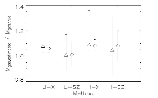
Figure 18: Comparison of median values and scatter of gas mass estimates inside $r_{500}$ for full SFF cluster sample (triangles) and cleaned SFF sample (diamonds) at z=0 for each of four methods: UTP-X-ray (U-X), UTP-SZE (U-SZ), isothermal X-ray (I-X), and isothermal SZE (I-SZ) as descibed in the text. From [49].

Fig. 18 shows the ratio of the measured mass to the actual mass for the star formation feedback catalog of simulated clusters for the four methods described above. The triangles are the full sample, whereas the diamonds are for samples which have been cleaned of highly distorted clusters resulting from recent mergers. The error bars enclose the 80% confidence range. As can be seen, cleaning the sample reduces the scatter considerably. Among the different methods, the X-ray measurements yield the smallest scatter, but overestimate the cluster masses by 5-10%. Conversely, the SZE-UTP measurements yield unbiased estimates the cluster mass, with somewhat more scatter. As shown in [49], the scatter in the SZE estimates decreases as the fitting radius is increased to $r_{200}$, while no improvement is seen in the X-ray estimates. This is to be expected since the X-ray emission is heavily core-weighted, while the SZE samples larger radii.

5.6 Conclusions

We have seen that galaxy clusters are sensitive cosmological probes provided their masses can be measured with precision. Both analytic estimates and numerical simulations show that the evolution of their comoving number density is sensitive to cosmology. With improvements in X-ray observations and impending large area surveys to detect clusters via the SZE, it is paramount to assess the accuracy to which cluster masses can be obtained observationally. Based on our catalogs of simulated clusters using adaptive mesh refinement, we find that gas masses can be measured to $\sim$10% accuracy with 80% confidence. Our study ignores instrumental or other observational effects. These limits in precision are a direct result of the deviation of the simulated clusters from simple assumptions about their physical and thermodynamic properties, dynamical state, and sphericity. Comparing a variety of methods, we find that SZE methods assuming a UTP produce the smallest scatter when estimating masses from a raw sample of clusters. Cleaning the cluster sample of obvious mergers does not improve the SZE estimates much, but improves the X-ray estimates substantially. As a practical matter, we find SZE methods are superior for mass estimation of large samples of clusters out to high redshift. This is particularly true if the cutoff radius is the virial radius, as this has the effect of smoothing out any boosting effects in the cluster core due to mergers.

Comparing mass estimates from our four catalogs, we find that our conclusions are insensitive to assumed baryonic physics, except for the cooling sample, which yields unrealistic-looking clusters. Mass estimates derived from the cooling sample are systematically high (50-100%) despite excising the overluminous X-ray core. Reasons for this are discussed in detail in reference [49]. We conclude that cool core clusters are poor candidates for precision mass estimation, in disagreement with previous studies [61].

- [1] \BYCarlstrom, J., Holder, G, & Reese, E. \INAnn. Rev. Astron. Astrophys.406432002.
- [2] \BYSpringel, V., White, S. et al. \INNature4356292005
- [3] \BYRosati, P., Borgani, S., & Norman, C. \INAnn. Rev. Astron. Astrophys.405392002.
- [4] \BYDodelson, S. \TITLEModern Cosmology, (Academic Press, Amsterdam), 2003.
- [5] \BYPerlmutter, S. \INPhysics TodayApril 200353
- [6] \BYSpergel, D. et al. \INApJS1481752003.
- [7] \BYBahcall, N. A.; Ostriker, J. P.; Perlmutter, S.; Steinhardt, P. J. \INScience28414811999
- [8] \BYTegmark, M. et al. \INApJ6067022004.
- [9] \BYWhite, S, Efstathiou, G., & Frenk, C. \INMNRAS2621023, 1993.
- [10] \BYKolb, E. & Turner, M. \TITLEThe Early Universe, (Addison-Wesley, Redwood City, CA), 1990.
- [11] \BYKomatsu, E. et al. \INApJS1481192003.
- [12] \BYPadmanabhan, T. \TITLEStructure Formation in the Universe, (Cambridge University Press, Cambridge), 1994.
- [13] \BYBryan, G. & Norman, M. \INApJ495801998.
- [14] \BYKaiser, N. \INMNRAS2223231986.
- [15] \BYBinney, J. & Tremaine, S. \TITLEGalactic Dynamics, (Princeton University Press, Princeton, USA), 1987.
- [16] \BYPress, W. & Schechter, S. \INApJ1874251974.
- [17] \BYWhite, S. D. M. \TITLECosmology and Large Scale Structure: Proceedings of Les Houches Summer School, R. Schaeffer et al., editors, (Elsevier, Amsterdam), 1996.
- [18] \BYEke, V., Cole, S. & Frenk, C. \INMNRAS281703
- [19] \BYNorman, M. L. \TITLEMatter and Energy in Clusters of Galaxies, ASP Conference Series Vol. 301, S. Boyer & C.-Y. Hwang, eds., (Astronomical Society of the Pacific, San Francisco), p. 419, 2003.
- [20] \BYFrenk, C. et al. \INApJ5255541999
- [21] \BYKatz, N., Weinberg, D. & Hernquist, L. \INApJS105191996
- [22] \BYSpringel, V., Yoshida, N., & White, S. \INNewA6792001
- [23] \BYBryan & Norman, M. \TITLEComputational Astrophysics; 12th Kingston Meeting on Theoretical Astrophysics, D. A. Clarke and M. Fall, editors, ASP Conference Series # 123, 1997.
- [24] \BYKravtsov, A., Klypin, A., & Kokhlov, A. \INApJS111731997
- [25] \BYTeyssier, R.. \INAstron. Astrophys.3853372002
- [26] \BYO’Shea, B. et al. \TITLEAdaptive Mesh Refinement–Theory and Applications, T. Plewa et al., eds., Springer Lecture Notes in Computational Science & Engineering, (Springer, Berlin), 2005.
- [27] \BYSpringel, V. et al. \INMNRAS3287262001
- [28] \BYAnninos, P. et al. \INNewA22091997
- [29] \BYPonman, T., Cannon, D. & Navarro, J. \INNature3971351999
- [30] \BYEfstathiou, G. et al. \INApJS572411985
- [31] \BYCouchman, H. \INApJL368L231991
- [32] \BYBarnes, J. & Hut, P. \INNature3244461986
- [33] \BYWarren, M. & Salmon, J. \INComp. Phys. Comm.872661995
- [34] \BYXu G. \INApJS983551995
- [35] \BYEvrard, A. \INMNRAS2359111988.
- [36] \BYKravtsov, A., Klypin, A. & Hoffman, Y. \INApJ5715632002
- [37] \BYKang, H. et al. \INApJ42811994
- [38] \BYBryan, G. et al. \INApJ4284051994.
- [39] \BYBorgani, S. et al. \INMNRAS34810782004
- [40] \BYBerger, M. & Colella, P. \INJ. Comp. Phys.82641989
- [41] \BYR. Hockney and J. Eastwood \TITLEComputer Simulation Using Particles, (McGraw Hill, New York), 1988.
- [42] \BYP. Colella and P. R. Woodward \INJ. Comp. Physics541741984
- [43] \BYW. Y. Anninos & M. L. Norman \INApJ4294341994
- [44] \BYCen, R. & Ostriker, J. \INApJ4174041993
- [45] \BYNavarro, J., Frenk, C. & White, S. \INApJ4625631996
- [46] \BYMotl, P. et al. \INApJL623L632005
- [47] \BYLoken, C. et al. \INApJ5795712002
- [48] \BYMotl, P. et al. \INApJ6066352004.
- [49] \BYHallman, E. et al. \TITLEpreprint, astro-ph/0509460
- [50] \BYVikhlinin, A. et al. \INApJ6286552005
- [51] \BYAscasibar, Y. et al. \INMNRAS3467312003
- [52] \BYDavis, M. et al. \INApJ2923711985
- [53] \BYEisenstein, D. & Hut, P. \INApJ4981371998
- [54] \BYHenry, J. P. & Arnaud, K. \INApJ3724101991
- [55] \BYBahcall, N., Fan, X. & Cen, R. \INApJ485L531997
- [56] \BYBryan, G. \INApJ544L12000
- [57] \BYVoit, M. & Bryan, G. \INApJ551L1392001
- [58] \BYRuszkowski, M., Bruggen, M. & Begelman, M. \IN6111582004
- [59] \BYda Silva, A. et al. \INMNRAS34814012004
- [60] \BYBuote, D. A. \INApJ5391722000
- [61] \BYAllen, S. & Fabian, A. \INMNRAS297L571998
- [62] \BYMarkevitch, M. et al. \INApJ503771998
- [63] \BYDe Grandi, S. & Molendi, S. \INApJ5671632002
- [64] \BYFabian, A. C. \INARAA322771994