Turbulence in the Solar Atmosphere: Manifestations and Diagnostics via Solar Image Processing

Abstract

Intermittent magnetohydrodynamical turbulence is most likely at work in the magnetized solar atmosphere. As a result, an array of scaling and multi-scaling image processing techniques can be used to measure the expected self-organization of solar magnetic fields. While these techniques advance our understanding of the physical system at work, it is unclear whether they can be used to predict solar eruptions, thus obtaining a practical significance for space weather. We address part of this problem by focusing on solar active regions and by investigating the usefulness of scaling and multi-scaling image processing techniques in solar flare prediction. Since solar flares exhibit spatial and temporal intermittency, we suggest that they are the products of instabilities subject to a critical threshold in a turbulent magnetic configuration. The identification of this threshold in scaling and multi-scaling spectra would then contribute meaningfully to the prediction of solar flares. We find that the fractal dimension of solar magnetic fields and their multifractal spectrum of generalized correlation dimensions do not have significant predictive ability. The respective multifractal structure functions and their inertial-range scaling exponents, however, probably provide some statistical distinguishing features between flaring and non-flaring active regions. More importantly, the temporal evolution of the above scaling exponents in flaring active regions probably shows a distinct behavior starting a few hours prior to a flare and therefore this temporal behavior may be practically useful in flare prediction. The results of this study need to be validated by more comprehensive works over a large number of solar active regions. Sufficient statistics may also establish critical thresholds in the values of the multifractal structure functions and/or their scaling exponents above which a flare may be predicted with a high level of confidence.

guessConjecture

1 Introduction

The magnetized solar atmosphere can be viewed both locally (solar active regions) and globally as an externally driven, dissipative, nonlinear dynamical system. The evolution of the system is largely dictated by the configuration of the magnetic field vector, which is subject to boundary-induced perturbations. These perturbations are either the emergence of additional magnetic flux from the solar interior or the shuffling caused by horizontal motions on the lower atmospheric boundary, the solar photosphere. Flux emergence and boundary flows, therefore, play the role of the external driver. The response of the system to external perturbations is nonlinear, consists of multiple manifestations, and occurs after a variable time delay with respect to the driving perturbation. This interval is necessary for the onset of acoustic, Alfvén, or magnetosonic, waves, and for the accumulation of electric currents in multiple locations within the magnetic configuration. The qualitative, first-order, description of the system is complete when dissipative processes are considered. These processes dissipate part of the non-potential magnetic energy stored in the magnetic structure in the form of electric currents. Currents are flowing both along and perpendicular to the magnetic field lines because these lines are twisted and clumped in braids, while localized shear between areas of different connectivity, either unipolar or multi-polar, creates additional current interfaces in the non-potential configuration. Dissipative events are abundant and can be intermittent, such as eruptions (flares and corona ejecta), or nearly continuous, such as the (homogeneous or inhomogeneous) heating processes in the solar chromosphere and corona. Although the energy content of the above processes is known and comes from the reservoir of free magnetic energy, solid evidence of their triggering via magnetic reconnection or wave damping and knowledge of their occurrence frequency are profoundly lacking.

Other key factors that preclude further understanding of solar magnetic fields are their filamentary nature (Parker 1979) and an ever-acting competition between two intrinsic tendencies: clustering and fragmentation of elemental magnetic flux tubes in the solar atmosphere (see, e.g., Abramenko and Longcope 2005). It appears that magnetic fragmentation is the prevailing tendency, with clustering dominating temporarily and locally during the formation of solar active regions. These entities occupy a small fraction of the photospheric surface at low latitudes, while the rest is occupied by small-scale magnetic flux elements.

To realize the physics of energy dissipation in the solar atmosphere the concept of turbulence has been proved a cornerstone in our understanding of solar magnetic fields. Most proposed solar dynamo mechanisms dealing with the generation of solar magnetic fields deep in the convection zone and the buoyant rise of magnetic flux tubes toward the atmosphere involve Kolmogorov’s theory of fluid turbulence (Cattaneo, Emonet, and Weiss 2003; Archontis, Dorch, and Nordlund 2003 and references therein). There is a sizable amount of evidence that turbulence is extended in the magnetically dominated solar atmosphere in the form of magnetohydrodynamic (MHD) turbulence. In essence, a turbulent evolution requires (1) a few large-scale, coherent, current-carrying magnetic structures, (2) ideal (non-dissipative) fragmentation of the free magnetic energy within an inertial range of length scales, and (3) a critical length scale below which magnetic resistivity sets in and releases part of the fragmented free energy. All of the above requirements are satisfied in modeled active regions and are supported by observations of actual solar active regions: the vector potential and the photospheric flows are organized in a few large-scale structures, while the electric current density and hence the magnetic free energy are distributed within numerous small-scale structures with linear sizes extending down to our present observational limit (e.g., Einaudi et al., 1996; Georgoulis, Velli, and Einaudi 1998; Chae 2001; Dmitruk et al., 2002). The first and the second process are known as an inverse and a direct cascade, respectively. Dissipation occurs when the length scale of the current structures becomes comparable to the Taylor microscale ($\sim 3\times 10^{3}\;cm$; Biskamp and Welter 1989), or even smaller ($\sim 20\;cm$) according to Kraichnan’s (1965) interpretation of a homogeneous and stationary MHD turbulence. Regardless of whether the above numbers are correct, the necessity of small spatial scales in order to achieve magnetic reconnection and subsequent current dissipation is most likely the reason why we lack evidence of flare and sub-flare triggering.

The phenomenology of turbulence in the solar atmosphere suggests a hierarchical self-organization of the physical parameters of the system. By self-organization we mean the reduction of the many parameters (degrees of freedom) exhibited by the complex solar magnetic structures to a small number of significant degrees of freedom that dictate the system’s evolution (see, e.g., Nicolis and Prigogine 1989). Assuming nonlinear self-organization directly contributes a number of powerful tools borrowed from the theory of nonlinear dynamical systems that can help assess the evolution of solar magnetic fields without necessarily elaborating on the detailed physics of the system. Such techniques are the percolation theory (Stauffer and Aharony 1994) and the concept of Self-Organized Criticality (SOC; Bak, Tang, and Wiesenfield 1987; Bak 1996 for a review) which have been successfully applied to solar physics. Percolation achieves self-organization via a competition of probabilities that regulate the clustering, fragmentation, and diffusion of solar magnetic fields and has reproduced the magnetic flux emergence and the formation of active regions in the Sun (Wentzel and Seiden 1992; Seiden and Wentzel 1996; Vlahos et al., 2002). SOC achieves self-organization without the finely tuned competing probabilities but using a critical threshold of a certain parameter (magnetic discontinuities, electric current density, etc.) whose excession, subject to external forcing, leads to an instability. According to local situation at the vicinity of the instability, a cascade of similar instabilities may occur as a result of the initial event as a domino-effect- or an avalanche-type process. SOC has described the triggering of solar flares and has provided a distinction between flares and sub-flares based on the size of the resulting avalanches (Lu and Hamilton 1991; Lu et al., 1993; Vlahos et al., 1995; Georgoulis and Vlahos 1996; 1998). Large avalanches correspond to flares, while small avalanches or nearly single events correspond to microflares or nanoflares, respectively. Notice, nonetheless, that the analogy between turbulence and SOC is imperfect in that the creation of an avalanche of elementary instabilities is yet to be definitively demonstrated in a turbulent simulation (Charbonneau et al., 2001). Reversely, it has been shown that the large, well-observed, solar flares can only be achieved by means of a SOC-type avalanche process which relaxes a large number of localized elementary instabilities (Vlahos and Georgoulis 2004).

A necessary but not sufficient condition for self-organization is the spatial and temporal self-similarity in the studied system. Self-similarity means that the system’s behavior does not depend on the temporal and spatial scales present: a magnification of an active-region plage, for example, reveals additional complex structure in small scales provided that the spatial resolution of the observing instrument is sufficient. Spatial self-similarity is a consequence of the filamentary nature of solar magnetic fields. In addition, the magnification of the temporal X-ray profile of a flare reveals additional temporal structure of the emission. If a critical threshold is involved in a self-similar (fractal) process, then spatial and temporal intermittency are also expected: intense X-ray flare emission is obtained within a very short interval compared to typical time scales of the evolution in the source active region, while the flaring volume is small compared to the volume of the active region regardless of the flare size. Intermittency and self-similarity can be measured and monitored via an array of image processing techniques, such as multi-scaling analysis of fractal and multi-fractal structures, image contrast enhancement, and pattern recognition. As diverse as they may appear, these techniques help understand and quantify the turbulence and intermittency present in the solar atmosphere. Therefore, they help understand the system at work in a way that complements the traditional approaches of solar physics. Numerous models and observational works have revealed the fractality and multi-fractality of active regions and their components (sunspots, plages), of small-scale magnetic concentrations in the “Quiet” Sun, and of the white-light magneto-convection (granulation and supergranulation) patterns (e.g., Roudier and Muller 1987; Lawrence 1991; Schrijver et al., 1992; Janßen, Vögler, and Kneer 2003). These studies have updated our knowledge of solar magnetic fields by showcasing the tremendous complexity exhibited by the processes at work. We have also learned that a possibly self-organized system can be very complex in its response, despite the few degrees of freedom that dictate this response. Despite these advances, however, the contribution of the various image processing techniques in understanding specific properties of the system with practical interest is controversial and far from clear: for example, although we can detect the buildup of magnetic flux and electric currents in an active region via image processing, we cannot predict when, where, or whether a major eruption will occur. Several conflicting accounts appear in the literature but, to our best knowledge, the predictive ability of image processing techniques has not been comprehensively investigated yet.

In this paper we acknowledge this problem and we suggest ways to tackle it by focusing on the multi-scaling properties of solar magnetic fields. Applications with practical space weather interest include flare and coronal mass ejection (CME) prediction. We will hereby focus on solar active regions (ARs) so we focus on flare, rather than CME, prediction, as the relationship between CMEs and the “source” ARs is unclear. In view of the observed intermittency of the solar flare phenomenon, our suggestion is to uncover likely critical thresholds of fractal and multifractal parameters whose excession might cause the triggering of a flare. We investigate whether this can be achieved by the existing array of image processing techniques and having the turbulent physics of the system in mind. In Section 2 we review some of the existing scaling and multi-scaling image processing techniques. In Section 3 we illustrate the possible significance of these techniques in flare prediction. In Section 4 we summarize the discussion and present our conclusions.

2 Understanding and Quantifying Turbulence via Image Processing

2.1 Flaring and Subflaring Activity

Although much of the image processing applied to solar physics has been focused on solar magnetic fields (Section 2.2), numerous studies have revealed the intermittent and self-similar nature of the energy release process in actual dissipative structures. Pattern recognition of energy release events has been applied to active-region X-ray bright points and transient brightenings (e.g., Shimizu 1995), extreme ultraviolet (EUV) bright points (Aletti et al., 2000; Benz and Krucker 2002; Aschwanden and Parnell 2002 and references therein), and off-band $H\alpha$ bright points, otherwise known as Ellerman bombs (EBs; Georgoulis et al., 2002). To our knowledge, such analyses have not been applied to full-scale flares observed in X-rays on in EUV wavelengths and we believe that a such study is long overdue. The identification of the emitting areas in the above works allows statistical studies in terms of the events’ area, duration, intensity and, in some cases, calculated energy content. Given a statistically sufficient number of events, one may construct the probability distribution function (PDF) for each of the above parameters. These PDFs invariably show well-defined power laws which underline the self-similar nature of the energy release process. Intermittency is also evident since the total area occupied by the emitting structures at any given time is small compared to the observational field of view. Examples of pattern recognition in subflaring activity are given in Figure 1. Although the existence of power laws is universal in flares and subflares, the value of the power-law index for the total-energy PDF for subflares is strongly debated. This value has implications on the heating efficiency of subflares in the solar atmosphere (see, e.g., Hudson 1991). In any case, the self-similar and intermittent nature of the energy release process causing the power-law PDFs appears beyond question.

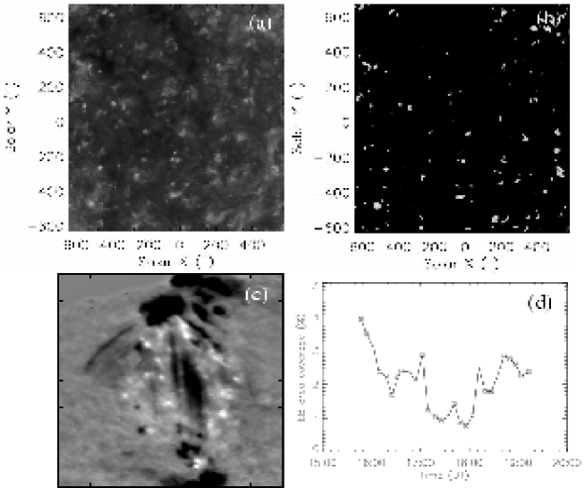
Figure 1: Pattern recognition in solar images of subflares: (a) Quiet Sun image from SoHO/EIT showing numerous EUV bright points, and (b) These bright points identified and singled out (from Alletti et al., 2000). (c) Off-band $H\alpha$ image from the Flare Genesis Experiment (FGE) showing numerous Ellerman bombs (EBs). Tic mark separation is $10^{\prime\prime}$. (d) Total area coverage of EBs normalized over the total field of view area for the entire FGE observations on January 25, 2000. The small percentage of total area coverage illustrates the intermittency of the EB phenomenon.

To quantify the degree of self-similarity in solar images such as those of Figure 1, one may calculate the fractal dimension of the energy release patterns. A such study has been performed for EBs by Georgoulis et al., (2002). They utilized a convenient box-counting method of measuring the fractal dimension (e.g., Mandelbrot 1983), as follows: Each off-band $H\alpha$ image (Figure 1c) is covered by a two-dimensional uniform and rectangular grid consisting of boxes with linear size $\lambda$. If the field of view has a linear size $L$, then it is covered by $(L/\lambda)^{2}$ boxes with dimensionless area $\varepsilon^{2}$, where $\varepsilon=(\lambda/L)$. Out of the $(L/\lambda)^{2}$ boxes, one then counts the number $N(\lambda)$ of boxes that contain at least part of an EB. Then, by varying $\lambda$, or, equivalently, the dimensionless area $\varepsilon$ of each box, one may study the variability of $N(\lambda)$ vs. $\lambda$ or $\varepsilon$. One obtains

$$N(\varepsilon)\propto({{1}\over{\varepsilon}})^{\mathcal{D}}\;\;,$$ (1)

where $\mathcal{D}$ is the (box-counting) fractal dimension of EBs. Other definitions of the fractal dimension can also be found in the literature, but adopting any one of them is sufficient to show whether a studied structure is fractal or not. The value of $\mathcal{D}$ can be at most equal to the Euclidean dimension of the image space for non-fractal structures. In our two-dimensional images, $\mathcal{D}=2$ would imply a spatially homogeneous, non-fractal, event distribution, while $\mathcal{D}<2$ would imply a fractal structure. The smaller the fractal dimension, the stronger the fragmenting tendency of the structures. For $\mathcal{D}<1$ in a two-dimensional image one obtains “dust fractals” with a dominant fragmentation tendency that precludes any mid- or large-scale structure clustering.

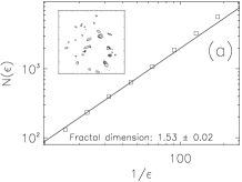
Figure 2: Fractal analysis of the energy release process in EBs (from Georgoulis et al., 2002): (a) The calculation of the box-counting fractal dimension $\mathcal{D}$ for a given off-band $H\alpha$ image, shown in the inset. (b) The calculated fractal dimensions for all $H\alpha$ images and for a given contrast threshold $I_{c_{0}}$. The average fractal dimension for that threshold is shown by the dashed line. (c) The dependence of the average fractal dimension with the contrast threshold.

An example of the above analysis in EBs shows that (i) the spatial distribution of the released energy is clearly fractal (Figure 2a), (ii) the fractal dimension varies around a well-defined average value for a given contrast threshold used to identify EBs (Figure 2b), and (iii) this average fractal dimension depends monotonically on the value of the threshold (Figure 2c). Dust fractal structures are obtained only for the most stringent threshold used, but this threshold is probably too restrictive, so despite the magnetic fragmentation intrinsic to the EB triggering process, EBs do tend to organize themselves in clusters. The physical interpretation of this result lies in the triggering locations of EBs and is explained in detail by Georgoulis et al., (2002). Despite the unambiguous fractality of EBs, however, we notice that a quantitative analysis of their fractal dimension is essentially threshold-dependent. This is the case for other types of sub-flaring activity, as well, and presents a problem in the analysis unless one has a physically sound reason behind the choice of a given threshold.

2.2 Solar Magnetic Fields

The majority of solar image processing has been applied to solar magnetic fields. The observed large-scale, persisting, photospheric magnetic flux accumulations that comprise solar ARs allow a detailed study in the course of time. Numerous works have shown that the active-region magnetic fields are self-similar structures, with area PDFs obeying well-defined power laws and with a fractal dimension ranging between $\sim 1.2$ and $\sim 1.7$ (see, e.g., Harvey 1993; Harvey and Zwaan 1993; Meunier 1999; 2004; Janßen, Vögler, and Kneer 2003 and references therein). The value of the fractal dimension depends on whether the structures themselves or their boundaries are box-counted. Fractal dimensions in solar magnetic fields are typically calculated using the box-counting technique discussed in Section 2.1. Nevertheless, the analysis has been pursued even further, to the concept of multifractality: it is well-known that an AR, for example, includes multiple types of structures such as different classes of sunspots, plages, emerging flux sub-regions, etc. The physics behind the formation and evolution of each of these structures is not believed to be identical, so the impact and the final outcome of turbulence in each of these configurations should not be the same. For each type of structure being a different fractal, an AR is then comprised by an ensemble of fractals, so it is a multifractal structure. The fractal dimension of a multifractal set is the maximum fractal dimension of the fractal subset that comprise the multifractal (Mandelbrot 1983). Numerous studies have revealed the multifractality of solar ARs, but also of the Quiet-Sun magnetic fields (e.g., Lawrence, Ruzmaikin, and Cadavid 1993; Cadavid et al., 1994; Lawrence, Cadavid, and Ruzmaikin 1996; Abramenko et al., 2001; Abramenko et al., 2002).

Various constructions of multi-scaling, or multifractal, spectra, can be used to quantify the multifractal character of solar magnetic fields. In the following, we briefly summarize some of these techniques:

2.2.1 Generalized correlation dimensions

The spectrum of generalized correlation dimensions can be derived for both timeseries and images (Vlahos et al., 1995; Georgoulis, Kluiving, and Vlahos 1995). One covers the observed magnetic flux image of size $L$ with a uniform rectangular grid consisting of elementary boxes with size $\lambda$ and dimensionless size $\varepsilon=(\lambda/L)$, as discussed in Section 2.1. One then finds the normalized magnetic flux $\tilde{\Phi}_{i}=(\Phi_{i}/\Phi_{tot})$; $i\equiv 1,...,(N/\lambda)$, for each of the boxes $i$, where $\Phi_{tot}$ is the total magnetic flux present in the field of view. Since $\sum_{i}\tilde{\Phi}_{i}=1$, each normalized flux $\tilde{\Phi}_{i}$ can be called a probability. In case of a multifractal AR, the weighted sum of probabilities $\sum_{i}\tilde{\Phi}_{i}^{q}(\varepsilon)$, raised to the power $q$ scales with $q$ as follows:

$$\sum_{i}\tilde{\Phi}_{i}^{q}(\varepsilon)\propto\varepsilon^{(q-1)D(q)}\;\;,$$ (2)

where $D(q)$ corresponds to the generalized Renyi dimensions. The “selector” $q$ is generally a real number, although negative values lack a physical interpretation. The function $D(q)$ is typically a decreasing function of $q$ for $q>0$. For $q=0$ one obtains the fractal dimension $\mathcal{D}=D(0)$ of the multifractal, while $D(n)$ for $q=n$ corresponds to the correlation dimension between $n$ neighboring flux accumulations, bounded within a box of size $\lambda$. If $D(n)<2$, where $2$ is the Euclidean dimension of the image, then there is correlation (that is, interaction or clustering) between the neighboring flux accumulations. The stronger the decrease of $D(q)$ for increasing $q$, the stronger the multifractal character of the magnetic flux accumulation. This is because $D(q)$ relates to the $q-$tuplet correlation integral $C_{q}(\varepsilon)$ as follows (Hentschel and Procaccia 1983):

$$D(q)={{logC_{q}(\varepsilon)}\over log\varepsilon}\;\;.$$ (3)

2.2.2 Structure functions

The structure function spectrum (Frisch 1995) has been applied to solar magnetic fields by Abramenko et al., (2002; 2003) in order to quantify the degree of intermittency in solar ARs. Instead of box-counting, one now introduces a characteristic displacement $\mathbf{r}$, called the separation vector, and defines a structure function

$$S_{q}(r)=\langle\mid\Phi(\mathbf{x}+\mathbf{r})-\Phi(\mathbf{x})\mid^{q}\rangle\;\;,$$ (4)

where the selector $q$ is also a real, preferably positive, number. The notation $\langle P\rangle$ corresponds to a spatial average of the quantity $P$ over the field of view. In case of an intermittent, multifractal, magnetic flux concentration, $S_{q}(r)$ exhibits a power-law dependence on $r$ within a certain range of displacements, namely,

$$S_{q}(r)\propto r^{\zeta(q)}\;\;,$$ (5)

where $\zeta(q)$ is the exponent of the structure function. In the absence of intermittency there is a linear relation $\zeta(q)=(q/3)$ between $\zeta(q)$ and $q$, but in actual, intermittent, solar magnetic fields the relation between $\zeta(q)$ and $q$ is either nonlinear or it departs significantly from the above linear slope. The power-law regime of $S_{q}(r)$ in which $\zeta(q)$ is measured extends between, say, $r=r_{1}$ and $r=r_{2}$, $r_{1}<r_{2}$, and can be interpreted as the inertial turbulent range where free magnetic energy fragments ideally and becomes distributed in successively smaller structures. The maximum limit $r_{2}$ probably refers to the maximum size of a magnetic structure that can participate in the inertial-range fragmentation, while the minimum limit $r_{1}$ refers to the breakdown of the inertial range and the onset of dissipation and subsequent release of free magnetic energy.

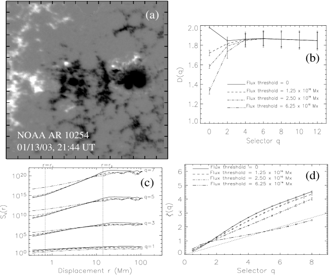
Figure 3: Multi-scaling spectra of NOAA AR 10254 observed by the IVM: (a) The measured line-of-sight magnetic field in the AR. The pixel size of the IVM image is $0.55^{\prime\prime}$, or $\sim 0.4\;Mm$. Tic mark separation is $20^{\prime\prime}$. Magnetic field values have been saturated at $700\;G$. North is up; west is to the right. (b) The spectrum $D(q)$ of the generalized correlation dimensions for various selectors $q$. Various magnetic flux thresholds have been used in the calculation. (c) The structure function spectrum $S_{q}(r)$ for various displacements $r$ and selectors $q$. The same flux thresholds with b have been used. The two parallel dotted lines indicate the common turbulent inertial range for all $q$. (d) The structure function exponents $\zeta(q)$ for various $q$ and flux thresholds. The dotted straight line corresponds to the non-intermittent turbulent case $\zeta(q)=(q/3)$.

An example of calculation of multi-scaling spectra in solar ARs is given in Figure 3. The subject is NOAA AR 10254 observed by the Imaging Vector Magnetograph (IVM; Mickey et al., 1996) of the University of Hawaii on 01/13/03. The entire magnetic field vector has been measured by the IVM, so the analysis has been applied to the total magnetic flux in the AR. Figure 3a shows the measured line-of-sight magnetic field. In Figure 3b we show the spectrum $D(q)$ of the generalized correlation dimensions for various $q$ and for various magnetic flux thresholds in the image. These thresholds are $(0,\;1.25\times 10^{16},\;2.5\times 10^{16},\;6.25\times 10^{16})\;Mx$ and correspond to total magnetic field thresholds $(0,100,200,500)\;G$ per pixel, respectively. We notice that $D(q)$ is practically independent from the flux threshold for $q\geq 2$. Only the fractal dimension $D(0)$ is sensitively threshold-dependent, as also found in Section 2.1 (Figure 2c) for sub-flaring activity. Therefore, the multifractal $D(q)$ spectrum is a more robust way of studying solar ARs than simply considering the fractal dimension. For $q\geq 4$ we notice that $D(q)$ decreases only slightly, if at all, indicating a weak multifractal character in the AR. In Figure 3c we show the structure functions $S_{q}(r)$ calculated for various $q$ and for the flux thresholds defined in Figure 3b. As with the $D(q)$ spectrum, the structure function $S_{q}(r)$ is fairly independent from the flux threshold used, except for the most stringent threshold of $6.25\times 10^{16}\;Mx$. Moreover, we notice that $S_{q}(r)$ becomes steeper for increasing $q$ and that the inertial range $r_{1}\leq r\leq r_{2}$ is easily discernible for any given $q$. The results of Figure 3c are in qualitative agreement with the results of Abramenko et al., (2002). In terms of a quantitative comparison, however, our inertial range is shifted to lower displacements with the lower limit $r_{1}$ extending practically down to the pixel size for $q\leq 3$. This suggests that magnetograms with better spatial resolution will reveal even smaller inertial-scale displacements. In Figure 3d we show the structure function exponents $\zeta(q)$ for various $q$ and using the four different flux thresholds. The dotted line indicates the expected non-intermittent turbulent spectrum $\zeta(q)=(q/3)$. Only for the most stringent flux threshold of $6.25\times 10^{16}\;Mx$ does the $\zeta(q)$ curve resemble the non-intermittent curve. This suggests that most of the intermittency in the AR resides in relatively weak magnetic fields $B<500\;G$. We also notice that $\zeta(q)$ increases nearly monotonically with increasing $q$, without reaching an apparent saturation value. According to Abramenko et al., (2003), this reflects a non-flaring period for the AR. We will return to this issue in Section 3.

Other examples of multi-scaling techniques embedded in solar image processing include the construction of the wavelet power spectrum. Wavelets have been used for diverse purposes but most notably to identify oscillatory wave modes in the solar chromosphere (e.g., McIntosh and Smillie 2004; Tziotziou, Tsiropoula, and Mein 2004); transition region (e.g. De Pontieu, Erdélyi, and de Wijn 2003), and the corona (e.g. De Moortel and Hood 2000). Wavelets have also been applied to solar magnetic fields although in a rather global manner, aiming to explain large-scale, universal, solar periodicities, such as the sunspot index and the nature of the 11-year solar cycle (Polygiannakis, Preka-Papadema, and Moussas 2003). These tasks lie beyond the scope of the present study and therefore wavelets will not be discussed further.

3 Tactical to Practical: Solar Image Processing with Space Weather Applications

We will now examine whether the techniques discussed in Section 2 can be useful for flare prediction. In the Introduction we mentioned that flares exhibit intermittency both in space and in time. Intermittency in a turbulent system prompts one to search for and identify critical thresholds of those few significant degrees of freedom that regulate the evolution of the self-organized system. Since solar ARs are invariably multifractal magnetic configurations with a variable degree of multifractality, it would be interesting to investigate critical thresholds in fractal and multifractal diagnostics that may distinguish flaring from non-flaring ARs. Such studies require large samples of ARs to ensure sufficient statistics, but we will attempt to identify promising avenues of further research even with a limited sample of ARs.

3.1 Fractal Diagnostics

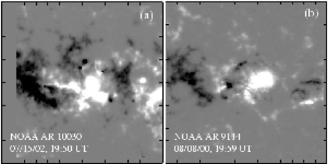
Figure 4: A fractal dimension comparison between a flaring and a quiescent solar AR. Both ARs have been observed by the IVM. The fractal analysis in box ARs has been performed using a flux threshold of $1.25\times 10^{16}\;Mx$. (a) NOAA AR 10030, which gave a X3 and a M1.8 flares during the IVM observations. (b) NOAA AR 9114, with no associated flaring activity. Tic mark separation in (a) and (b) is $20^{\prime\prime}$. North is up; west is to the right in both images. (c) Various measures of the fractal dimension for NOAA AR 10030. (d) Various measures of the fractal dimension for NOAA AR 9114.

A flaring and a quiescent ARs observed by the IVM are given in Figures 4a and 4b, respectively. NOAA AR 10030 gave two major flares, namely a X3 and a M1.8, during the IVM observing interval. NOAA AR 9114 gave no flares, not even C-class events, on the particular day of the observations. The two ARs are distinctly different in terms of magnetic complexity and flow patterns, and show a factor of two difference in total magnetic flux ($\sim 8\times 10^{22}\;Mx$ and $\sim 4\times 10^{22}\;Mx$ for ARs 10030 and 9114, respectively). We have measured various fractal dimensions for the two ARs over the course of the IVM observations. Since the values of the fractal dimension are threshold-dependent (Figures 2c, 3b), we have chosen the same magnetic flux threshold of $1.25\times 10^{16}\;Mx$ ($100\;G$ per pixel) for both ARs and at any given time. We have measured the fractal dimension of the magnetic patches and their boundaries, both using the unsigned total magnetic flux and discriminating between positive and negative magnetic polarity. Our results are given in Figures 4c and 4d for ARs 10030 and 9114, respectively. By inspecting and comparing the two plots we reach the following conclusions:

1. The values of the various fractal dimensions fluctuate slightly in the course of time, around a well-defined average value. This is the case for both ARs. Moreover, there are no measurable changes in any fractal dimension that reflect the triggering of the two flares in AR 10030. The onset times of the flares were 20:02 UT and 21:30 UT for the X3 and the M1.8 flare, respectively.

2. The fractal dimension measured when both the interior and the boundaries of the patterns are box-counted is higher than that measured from only the boundaries of the patterns. Discriminating between the two polarities does not alter this conclusion. Both ARs give boundary fractal dimensions varying between $1.1$ and $1.3$. AR 10030, however, gives larger fractal dimensions when boundaries and interiors are box-counted.. In AR 10030 the values of the fractal dimension range between $1.5$ and $1.7$, while in AR 9114 they vary between $1.3$ and $1.5$. This feature is not related to the flare productivity of AR 10030: this region is spatially more extended compared to AR 9114, so it occupies a larger fraction of the fixed IVM field of view. Since the interiors of the flux patterns are box-counted, there are more filled elementary boxes for AR 10030 than for AR 9114 which increases the fractal dimension. In view of this effect, which might lead to misinterpretation of the results, it appears safer to use the boundary fractal dimensions.

I general, we find no distinguishing feature in the measurement of the fractal dimension that can hint about the dramatically different activity levels in NOAA ARs 10030 and 9114. The values of the various fractal dimensions are similar for both ARs, while in cases where there is a difference it is not related to the flare productivity in the AR. Moreover, no noticeable changes in the fractal dimension occur before and after the flares. In addition, given the fact that the values of the fractal dimension depend sensitively on employed flux threshold, we conclude that the fractal dimension is not a useful means of distinguishing flaring from quiescent ARs, although it quantifies the degree of self-similarity in solar ARs. We cannot rule out the possibility that statistical patterns might be obtained when the fractal dimension is calculated for a large number of flaring and quiescent ARs, but this example here indicates that there might be little hope for that. The fractal dimension can be useful for other types of studies, nevertheless, such as those dealing with the different phases of the solar cycle. Meunier (2004) reports a significant variation of the fractal dimension between solar minimum and solar maximum. However, the objectives of space weather forecasting are different and essentially focused on short- and mid-term predictions of the eruptive potential in solar ARs, rather than on long-term predictions of the order of the solar cycle.

3.2 Multifractal Diagnostics

Let us now investigate whether multifractal spectra can help one distinguish between flaring and quiescent ARs. For this task, we have chosen a sample of six ARs observed by the IVM. Three of these ARs, namely NOAA ARs 10030, 8210, and 9165, gave at least M-class flares on the day of the IVM observations and they are considered “flaring” ARs. The remaining three ARs, namely NOAA ARs 9114, 8592, and 10254, are not associated with M-class or larger flares on the day of the observations and they are considered “quiescent” ARs. Although we have shown in Section 2.2 that the multifractal spectra do not depend sensitively on the employed flux threshold, for comparison purposes we use the same threshold for all six ARs. This flux threshold is $1.25\times 10^{16}\;Mx$.

Figure 5: Generalized correlation dimensions $D(q)$ for various selectors $q$ and for a sample of flaring (solid curves) and non-flaring (dashed curves) ARs.

We first calculate the generalized correlation dimensions $D(q)$ for all ARs and for various selectors $q$. The results are shown in Figure 5. It is evident that there is no distinguishing feature between the flaring and the non-flaring ARs, since the shape of the $D(q)$ spectra and the $D(q)$-values are similar, within error bars, for both types of ARs. The exception from this conjecture is AR 9165 with significantly lower $D(q)$-values compared to the other ARs. This implies that AR 9165 exhibits the strongest multifractal character and it is also a flaring AR. Nonetheless, we cannot definitively link the degree of multifractality with the flare productivity, since the other two flaring ARs do not show this feature. AR 9165 was not even the most flare-productive AR. On the day of the observations AR 9165 gave a M2 flare, while AR 10030 gave a X3 and a M1.8 flare. In conclusion, the construction of the generalized correlation dimensions $D(q)$ is not particularly useful in identifying potentially flaring ARs.

We then calculate the structure functions $S_{q}(r)$ and their inertial-range scaling exponents $\zeta(q)$ for various selectors $q$ and displacements $r$. This is a very interesting test given that there are reports in the literature arguing that $S_{q}(r)$ and $\zeta(q)$ can provide clues for the flare productivity of solar ARs. In particular, Abramenko et al., (2002; 2003) report that (i) the $S_{q}(r)$ spectra are flatter for flare-productive ARs compared to quiescent ARs, and (ii) the shape of the $\zeta(q)$ spectrum deviates significantly from the linear non-intermittent case, $\zeta(q)=(q/3)$, for flaring ARs. The flattening of the $S_{q}(r)$ spectra and the nonlinear $\zeta(q)$ curve suggest an increase of intermittency and they are reported to occur in ARs prior to a solar flare.

Figure 6: Structure function calculations for a sample of flaring (solid curves) and non-flaring (dashed curves) ARs. (a) The structure functions $S_{3}(r)$ for $q=3$. The power-law regimes indicate the turbulent inertial range of the magnetic fragmentation process in the ARs. (b) The inertial-range scaling exponents $\zeta(q)$ of the structure functions $S_{q}(r)$ for various selectors $q$. The dotted straight line corresponds to the expected spectrum, $\zeta(q)=(q/3)$, in case of a non-intermittent turbulence.

The $S_{3}(r)$ values ($q=3$) for all chosen ARs are given in Figure 6a. Other values of the selector $q$ give similar results. We notice that, with the exception of AR 8210, the flaring ARs tend to have larger inertial-range values of $S_{3}(r)$ for a given $r$. It is not clear why AR 8210 does not follow this trend and we certainly cannot rule out the possibility of a random occurrence of this result given the limited sample of ARs. Nevertheless, it appears worthy to perform the same study for a much larger number of ARs aiming to investigate whether flaring ARs tend to give statistically larger values of $S_{q}(r)$ for given $q$ and $r$. The shape of the $S_{q}(r)$ spectrum does not appear to provide any other distinguishing feature between flaring and non-flaring ARs. In Figure 6b, on the other hand, we find that two out of three flaring ARs (ARs 10030 and 9165) show smaller $\zeta(q)$ exponents for $q\geq 4$ compared to the other ARs, suggesting that the $S_{q}(r)$ are flatter in their inertial range for these two cases. This is in agreement with Abramenko et al., (2002; 2003). AR 8210 again exhibits an unclear behavior with the values of $\zeta(q)$ being comparable to those of the quiescent ARs. Moreover, it is also troubling that AR 9165 gives the strongest nonlinear response for $\zeta(q)$ although it is not the most flare-productive AR. In qualitative agreement with Abramenko et al., (2002; 2003), on the other hand, the shape of the $\zeta(q)$ spectrum in flaring ARs deviates more from the non-intermittent linear case (dotted line) than in non-flaring ARs. This conclusion does not include the flaring AR 8210.

Summarizing, we generally confirm the results of Abramenko et al., (2002; 2003) but not without exceptions. Clearly, the proposed multi-scaling criteria cannot discriminate unambiguously between flaring and quiescent ARs and the diagnostics are not more profound for the most flare-productive ARs. The uncovered trends, however, make it worthy to study the $S_{q}(r)$ and $\zeta(q)$ spectra for a large number of subject ARs aiming to reveal statistical, probabilistic, patterns regarding the flare productivity in ARs. Our analysis suggests that emphasis should be placed on the following aspects:

1. The inertial-range values of the $S_{q}(r)$ spectra for a given $q$ (flaring ARs may tend to give larger $S_{q}(r)$),

2. The values of $\zeta(q)$ and the shape of the $\zeta(q)$ spectrum (flaring ARs may tend to give more nonlinear $\zeta(q)$ response with smaller values of $\zeta(q)$ for larger $q$).

If such patterns are statistically confirmed, the one might be able to define critical thresholds $S_{q;cr}(r)$ and $\zeta_{cr}(q)$ for $S_{q}(r)$ and $\zeta(q)$, respectively. Values $S_{q}(r)>S_{q;cr}(r)$ for given $q$ and $r$, as well as values $\zeta(q)<\zeta_{cr}(q)$ for a given $q$, might imply an enhanced likelihood of flaring events in an AR.

We note in passing that the same sample of ARs has been used in different investigations of the flaring vs. the quiescent activity. In Georgoulis and LaBonte (2005) we provide more clear distinguishing features between flaring and non-flaring ARs based on the free magnetic energy and the total magnetic helicity budgets of the above sample of ARs.

A further important test is to examine the multifractal behavior of a flaring AR in the course of time and ideally before and after the flaring event(s). As discussed in Section 3.1, NOAA AR 10030 is appropriate for this task since it produced two flares during the IVM observing interval. The flare onset times were 20:02 UT and 21:30 UT for a X3 flare and a M1.8 flare, respectively. We selected 4 snapshots of the AR before the X3 flare (17:31 UT; 18:10 UT; 18:57 UT; and 19:50 UT) and 3 snapshots after the event (20:29 UT; 21:13 UT; and 22:04 UT). We carefully excluded from the analysis magnetograms obtained during the rising phase and the peak of the flares to avoid possible contamination of the polarization measurements from the white-light flare emission (see, e.g., Qiu and Gary 2003). Moreover, we used a fixed flux threshold for all magnetograms, equal to $1.25\times 10^{16}\;Mx$.

We first examined the temporal behavior of the generalized correlation dimensions $D(q)$. This test did not provide useful results. In fact the only result was a decrease of the $D(q)$ values after the X3 flare at 20:29 UT which, however, was insignificant and mostly kept within error bars. This implies that the degree of multifractality in the AR increased after the X-class flare. This increase, however, is not significant enough to overcome error bars and become useful for flare prediction.

Figure 7: Temporal multifractal analysis of the flaring NOAA AR 10030. (a) The structure functions $S_{3}(r)$, for $q=3$, for various times before and after the X3 flare (solid lines and dashed lines, respectively). (b) The temporal evolution of the inertial-range scaling exponents $\zeta(q)$ for various selectors $q$. The onset times of the two flares triggered in the AR are indicated by the two parallel dashed lines.

We then calculated the structure functions $S_{q}(r)$ and their inertial-range exponents $\zeta(q)$ as functions of time. The values of $S_{3}(r)$ for $q=3$ and for various displacements $r$ are given in Figure 7a. Similar results are obtained for other choices of $q$. From Figure 7a we notice that (i) there is no significant difference in the inertial-range values of $S_{q}(r)$ before and after the flares, and (ii) the inertial power-law regime flattens after the events. The effect is more discernible in Figure 7b and for $q\geq 2$, where the values of $\zeta(q)$ decrease after the events. As a result, the response of $\zeta(q)$ becomes more nonlinear after the flares, suggesting that the degree of intermittency in the ARs has been increased after the events. This stands in agreement with the results of Abramenko et al., (2002; 2003). The decrease of $\zeta(q)$ for a given $q\geq 2$ is beyond error bars and ranges from $\sim 4\%$ ($q=2$) to $\sim 20\%$ ($q=3.5$). We have performed the same test for the quiescent AR 9114 and we could not detect such changes of $\zeta(q)$ in the course of time. The temporal variation of $\zeta(q)$, therefore, can be used to identify flaring periods in an AR. To become even more practical for flare prediction, however, $\zeta(q)$ should also be able to identify pre-flare periods in solar ARs. From Figure 7b we notice an increase of $\zeta(q)$ before the X3 flare and for $q\geq 2$. This behavior suggests a pre-flare decrease of the intermittency in the AR and is discernible after 18:00 UT, that is $2\;hr$ before the X3 flare.

In conclusion, the temporal variation of $\zeta(q)$ in a flaring AR is probably the most useful multifractal diagnostic of imminent flaring activity. Further tests on large numbers of flaring and non-flaring ARs are required to substantiate this. The tale-telling signature for an imminent flare appears to be a significant increase in $\zeta(q)$ a few hours before the event followed by an also significant decrease of $\zeta(q)$ after the event. The sufficient statistics of a comprehensive analysis should be able to establish critical thresholds of the pre-flare increase of $\zeta(q)$ beyond which a flare might be safely predicted.

More multifractal indices can be defined as by-products of the multi-scaling analysis in solar ARs (see Abramenko et al., 2003 for examples) but one should focus on the right combination of simplicity and usefulness in the construction and practical use of a given index for space weather purposes. From this aspect, the inertial-range exponents $\zeta(q)$ of the structure functions $S_{q}(r)$ are probably the most appropriate multifractal diagnostics of flares, given their simple construction and sound physical justification.

3.3 Other Image Processing Techniques with Space Weather Applications

In this study we focused on image processing techniques directly stemming from the theory of nonlinear dynamical systems exhibiting intermittent self-organization. This is not the only image processing applied to solar data. Additional solar image processing techniques with an impact in space weather forecasting generally refer to two broad categories: (1) pattern recognition, and (2) contrast enhancement and difference imaging.

Pattern recognition techniques apply to active-region recognition and sunspot identification / classification on the visible solar disk (e.g. Turmon, Pap, and Mukhtar 2002; see also the web pages of the Active Region Monitor and the Max Millenium Program of Solar Flare Research), filament identification from $H\alpha$ images of the solar chromosphere (Bernasconi, Rust, and Hakim 2005; this volume), sigmoid recognition from soft X-ray images of the lower solar corona (LaBonte, Rust, and Bernasconi 2004), and CME recognition from white-light images of the outer corona (Robbrecht and Berghmans 2004 and in this volume). Sunspot and active-region identification is a prerequisite for the automatic application of the scaling and multi-scaling techniques discussed in the previous Sections and hence this task is an integral part of the solar research required for space weather forecasting. Equally important is the automatic, real-time, identification of CMEs. Filament and sigmoid recognition, on the other hand, can help understand the pre-launch phases of a CME. Although these techniques are not directly related to the theory of intermittent turbulence, there is a critical threshold that can place the CME prediction on a quantitative basis. This threshold comes from the helical structure of solar magnetic fields and the flux ropes that fuel a CME. If the aspect ratio $(L/R)$ of a, say, cylindrical flux rope is larger than a critical threshold $(L/R)_{cr}$, then the flux rope becomes kink-unstable and may erupt. In the above notation $L$ is the length of the flux rope and $R$ is the radius of the cylinder. Rust and Kumar (1996) have shown that $(L/R)_{cr}\simeq 5.4$. Measurement of the aspect ratios of X-ray sigmoids can be performed automatically and in real time. Moreover, the shape of filaments and sigmoids can reveal the sense of magnetic helicity (chirality) of the pre-eruption structure thus adding to the predictive ability of these pattern recognition techniques. The notion of a critical threshold provided by the theory of the kink instability fits nicely with the viewpoint that CMEs are caused by a loss of equilibrium in the solar atmosphere (see Forbes 2000 and references therein). The CME phenomenon is also characterized by temporal intermittency and self-similarity with the CME launch lasting only a few $hr$ and the PDFs of the CME kinetic energies obeying well-defined power laws (Vourlidas 2004; private communication). Therefore, it is conceivable that SOC models and fractal/multifractal diagnostic techniques may be developed in the future to study the CME initiation process.

Contrast enhancement and difference imaging apply to the detection of EUV transient dimmings that accompany the launch of a CME (e.g. Aschwanden 2005; this volume), the detection of Moreton waves, or “EIT waves”, following a flare and/or a CME (Thompson et al., 1999), and the sharpening of the white-light CME images observed by SoHO/LASCO (Stenborg and Cobelli 2003; Stenborg 2005; this volume). Transient dimmings accompanying the CME initiation are long known and frequently observed (e.g. Rust 1983). They are thought to correspond to the footpoints of the CME and the subsequent interplanetary flux rope (e.g. Kahler and Hudson 2001 and references therein). Therefore, their detection is of particular space weather importance. The physical nature of the EIT waves remains elusive (Zhukov and Auchére 2004) but their study, via the study of differences between consecutive EUV images, contributes to the construction of a consistent and comprehensive physical picture of the CME phenomenon. Regarding the sharpening of the CME images using, for example, wavelet techniques, we suggest that a semi-quantitative analysis of the magnetic helicity of CMEs can be performed, although it is questionable whether this analysis can be done automatically. In particular, one can arguably measure the amount of twist, via the length of the CME structure and the number of turns as they are revealed from the sharpened image, and the amount of writhe, thus estimating the total magnetic helicity of the structure. This estimation can be compared against the estimated helicity of the pre-CME sigmoids and filaments in order to understand which magnetic fields contribute to a CME. The latter is a completely open question, with the debate holding on whether CMEs are local events, i.e., they originate from single active-region magnetic fields/filaments, or global events, i.e., requiring an interaction between the active-region magnetic fields and the global solar dipole. Comparable helicities between the CME and the source sigmoid, for example, would point to a direct relationship between the CME and the X-ray coronal loop, while large discrepancies would suggest that CMEs are events with their magnetic structure contributed by the large-scale solar magnetic fields besides the source magnetic structure. CME image enhancement has already uncovered the rich structure of the CMEs’ magnetic configuration, but via this plausible research option we might be able to gain much more understanding of the CME triggering process.

4 Summary and Conclusions

Intermittent MHD turbulence is a key feature of magnetic fields, their evolution, and the associated eruptive activity in the Sun’s atmosphere. As a result, fractal and multifractal image processing techniques are applicable and can be used to quantify the degree of intermittency, self-similarity, and multifractality present in the system. While these multi-scaling techniques can advance our understanding of solar magnetic fields, it is questionable whether they can be used to predict eruptive activity such as solar flares and CMEs. This is because intermittency, self-similarity, and multifractality are so widespread in the solar magnetic fields that it is not clear whether the above techniques are appropriate to discriminate between different types (i.e. flare-productive and quiescent) magnetic configurations.

We address this question in the present study. In particular, we ask whether fractal and multifractal diagnostics can be of any predictive importance. We focus on the prediction of solar flares, rather than on CME prediction, because there are several open questions regarding the origin of CMEs that do not allow the zero-level understanding required to adjust multi-scaling techniques for their study. Prompted by the intermittency of the solar flare phenomenon and the overall self-organization of the solar magnetic fields we search for possible critical thresholds in the scaling and multi-scaling behavior of the nonlinear dynamical system which, if exceeded, can give rise to intermittent energy dissipation, namely, to a solar flare. To study flare-productivity in solar ARs we measure the fractal dimension, the multifractal generalized correlation dimensions, the multifractal structure functions, and their inertial-range scaling exponents of the photospheric magnetic flux comprising these ARs. Our results can be summarized as follows:

1. ] The calculation of the fractal dimension is not a particularly fruitful way to discriminate flaring from quiescent ARs. The value of the fractal dimension is sensitively threshold-dependent and is similar between the two different types of ARs. Moreover, care is required to the definition of the fractal dimension. When both the boundaries and the interiors of magnetic flux patterns are used in the measurement of the fractal dimension, then the results become dependent on the ratio between the spatial extent of the AR and the finite field of view. This can lead to misinterpretation of the results and in differences in the values of the fractal dimension that are not related to flaring activity. Therefore, we expect that the use of the fractal dimension for flare prediction purposes should be limited.

2. ] The calculation of the generalized correlation dimensions $D(q)$ is also not particularly useful. Flaring and non-flaring ARs tend to show similar values of $D(q)$. The gain in the use of the $D(q)$ spectrum is that it reveals the degree of multifractality of active-region magnetic fields. However, this does not appear to be a sensitive function of the flare productivity in solar ARs. Therefore, $D(q)$ spectra are not expected to improve our flare-forecasting ability.

3. ] The calculation of the structure functions $S_{q}(r)$ and their inertial-range exponents $\zeta(q)$ have provided some forecasting clues, but not without limitations. In particular, (i) flaring ARs tend to show larger inertial-range $S_{q}(r)$ values for given $q$ and $r$, (ii) flaring ARs tend to have flatter $S_{q}(r)$ spectra, that is, smaller $\zeta(q)$ values, for a given $q$, and (iii) flaring ARs tend to show more nonlinear $\zeta(q)$ curves than non-flaring ARs. These tendencies, nonetheless, have exceptions for both flaring and non-flaring ARs so a comprehensive statistical study relying on a large active-region sample is required. The result should be a statistical preference on the values of $S_{q}(r)$ and $\zeta(q)$ for flaring ARs which might improve our flare-forecasting ability.

4. ] An interesting result is found regarding the temporal evolution of the scaling exponent $\zeta(q)$ in a flaring AR. The values of $\zeta(q)$ appear to increase significantly a few $hr$ before the flare and decrease significantly after the event. This corresponds to a decrease of the intermittency in the active-region magnetic fields during the pre-flare phase followed by a subsequent increase of the intermittency in the post-flare phase. This result, however, is only based on a single example of a flaring AR with flares occurring during the observations, as compared to non-flaring ARs. Further study of more flaring ARs is obviously required. If confirmed, this trend might be of specific flare-predictive value.

To complete the discussion on the structure functions $S_{q}(r)$, we notice that a largely overlooked aspect of their analysis is the lower limit $r_{1}$ of their turbulent inertial range (Figure 3c). In several examples (Figures 6a, 7a) and for moderate selectors ($q\leq 2$), $r_{1}$ extends down to the instrument’s pixel size. This feature can be useful in future, high-resolution, magnetograms and can be used to identify the length scale where the breakdown of the turbulent inertial range occurs. This is the length scale where magnetic resistivity sets in or, in other words, the magnetic Reynolds number becomes small enough to allow dissipation of free magnetic energy via magnetic reconnection. Finding the true value of $r_{1}$ will allow testing of theoretical estimations and their respective physical backgrounds, such as the Taylor microscale or Kraichnan’s length scale of MHD turbulence. This development will hardly contribute to our space weather forecasting ability but it will advance our understanding of solar magnetic fields. The Solar-B mission will contribute very high-resolution space-based vector magnetograms in a few years. The quantitative study of turbulence and the flaring phenomenon in these magnetograms will certainly be a worthy task.