Cosmological Signatures of Interacting Neutrinos

Abstract

We investigate signatures of neutrino scattering in the Cosmic Microwave Background (CMB) and matter power spectra, and the extent to which present cosmological data can distinguish between a free streaming or tightly coupled fluid of neutrinos. If neutrinos have strong non-standard interactions, for example, through the coupling of neutrinos to a light boson, they may be kept in equilibrium until late times. We show how the power spectra for these models differ from more conventional neutrino scenarios, and use CMB and large scale structure data to constrain these models. CMB polarization data improves the constraints on the number of massless neutrinos, while the Lyman–$\alpha$ power spectrum improves the limits on the neutrino mass. Neutrino mass limits depend strongly on whether some or all of the neutrino species interact and annihilate. The present data can accommodate a number of tightly-coupled relativistic degrees of freedom, and none of the interacting-neutrino scenarios considered are ruled out by current data — although considerations regarding the age of the Universe disfavor a model with three annihilating neutrinos with very large neutrino masses.

I Introduction

We are in a remarkable era when cosmological data is both precise and abundant. Measurements of temperature and polarization fluctuations in the cosmic microwave background (CMB) radiation (e.g. WMAP ; ACBAR ; CBI ; CBIpol ), the matter power spectrum via galaxy surveys 2dF ; SDSS and the Lyman-$\alpha$ forest VHS04 ; lyman , the current and past expansion rate of the Universe via the Hubble Key Project HST and observations of Type Ia supernovae Supernovae respectively, and the abundance of light elements predicted by big bang nucleosynthesis (BBN) BBN all show striking consistency within the standard $\rm{\Lambda CDM}$ cosmological model. Robust bounds can be placed on the forms of matter and energy that constitute the Universe, and cosmology is now a powerful particle physics laboratory that constrains the properties of both the new dark-matter particles demanded by cosmological data (e.g. DarkMatterProperties ) and the familiar particles of the standard model of particle physics. In many cases these constraints would be difficult or impossible to obtain in any other way.

Neutrino physics is an excellent example. Cosmological techniques for probing neutrino properties rely upon detecting indirect signatures of the relic neutrino background, which complements the significant experimental and theoretical effort that is underway to understand the surprising physics of the neutrino sector. A particular focus of this effort has been to set limits on the mass and number density of relic neutrinos. In this work we instead focus on the cosmological signatures of neutrino interactions.

It is well known that the CMB can be used to constrain the number of light relativistic degrees of freedom (in addition to the photon) – conventionally parametrized as the effective number of neutrino species, $N_{\nu}^{\rm eff}$. A relative increase in the radiation density delays the epoch of matter-radiation equality, and leads to an enhanced Integrated Sachs-Wolfe (ISW) effect. Present CMB limits are $1.6\leq N_{\nu}^{\rm eff}\leq 7.1$ Nnu ; Pierpaoli . Big Bang nucleosynthesis (BBN) also constrains $N_{\nu}^{\rm eff}$, as additional radiation increases the expansion rate and alters the expected primordial abundance of helium. The current BBN bound is (up to various flavor dependent subtleties) $N_{\nu}^{\rm eff}<3.3-4$ BBN .

The standard cosmological model predicts $N_{\nu}^{\rm eff}\approx 3.04$, consisting of the three known neutrino species, plus a small correction that accounts for the neutrino heating from electron-positron annihilation and finite-temperature QED effects (e.g. Lopez:1998aq ). With only the three standard neutrino species, BBN constraints, combined with neutrino mixing, no longer permit the possibility of a significantly enhanced $N_{\nu}^{\rm eff}$ due to large chemical potentials degen . However, it is important to bear in mind that $N_{\nu}^{\rm eff}$ may include not only neutrinos, but any light particles that are thermally populated in the early universe. In models containing sterile neutrinos or other light relativistic degrees of freedom, the BBN limits may be substantially modified, and $N_{\nu}^{\rm eff}>3$ is still possible kneller . (In addition, $N_{\nu}^{\rm eff}<3$ can be obtained if the reheating temperature following inflation is low lowreheat .) Moreover, the relativistic energy density may evolve between the time of BBN and CMB decoupling, so $N^{\rm eff}_{\nu}|_{\rm BBN}$ and $N^{\rm eff}_{\nu}|_{\rm CMB}$ need not be the same quantity (e.g. chacko ; neutrinoless ).

In addition to the total relativistic energy density, cosmology can also be used to probe interactions in the neutrino sector. Neutrinos with only standard model couplings interact via the weak force, and decouple when $T\simeq 1$ MeV. At later times, they free-stream, and interact only via gravity. In this paper we investigate a class of models which feature extra, non-standard, neutrino interactions. In these models, neutrinos interact strongly with a new scalar boson, which is brought into thermal equilibrium though its coupling to the neutrinos. Rather than free-streaming, the neutrinos form a tightly coupled fluid with the new scalar.

These models generically have non-standard values for $N_{\nu}^{\rm eff}$, but perhaps more interestingly, the absence of neutrino free-streaming leaves a distinctive signature in the CMB. If the neutrinos are part of a tightly coupled fluid, they are fully characterized by density and velocity perturbations, and anisotropic stress is negligible. In hannestad ; trotta it was shown that the current Wilkinson Microwave Anisotropy Probe (WMAP) CMB measurements already have some sensitivity to this effect. This is significant because in addition to being able to infer the presence of relativistic degrees of freedom, we may now also be able to say something about the interactions of the particles which make up that relativistic energy density.

In this paper we address the question: how much relativistic energy density is there, and what fraction of it must consist of weakly interacting particles? We answer this question in general, and also in the context of specific models.

II Interaction Model

Although the results of our analysis are valid in a wider context than the interaction model we now describe, we examine in this section a simple physical model of non-standard neutrino interactions for illustrative purposes.

We consider the coupling of neutrinos to each other with bosons, through tree level scalar or pseudo-scalar couplings of the form

$${\cal L}_{\nu\phi}=h_{ij}\overline{\nu}_{i}\nu_{j}\phi+g_{ij}\overline{\nu}_{i}\gamma_{5}\nu_{j}\phi,$$ (1)

where the boson $\phi$ is taken to be light or massless. Such couplings arise in Majoron-like models, viable examples of which have been discussed in Ref. Models . Recently, these models have been investigated in the context of late-time phase transitions, whereby the neutrinos acquire their masses via a symmetry breaking phase transition at a low scale, which occurs late in the history of the universe chacko ; mohapatra . In order to be as model independent as possible, we assume the new couplings are fixed independently of the neutrino mass. We also make no distinction between $g$ or $h$ type couplings, nor between neutrinos and antineutrinos.

Existing bounds on these new couplings are extremely weak. For example, the solar neutrino SolarDecay and meson decay MesonDecay limits are $|g|\lesssim 10^{-2}$. Neutrinoless double beta decay sets a limit $g_{ee}<10^{-4}$ doublebeta , but does not constrain other elements of the coupling matrix $g_{\alpha\beta}$. Supernova constraints exclude a narrow (and model-dependent) range of couplings around $g\sim 10^{-5}$ Supernova . Even couplings which are much smaller than these limits can have significant cosmological consequences.

For a massless $\phi$ boson, scalar couplings could mediate long-range forces with possible cosmological consequences LongRange ; mckellar , while pseudo-scalar couplings mediate spin-dependent long-range forces, which have no net effect on an unpolarized medium. However, if the $\phi$ boson has even a tiny mass $H_{0}\ll m_{\phi}\ll 1$ eV the interaction is short ranged and insignificant over cosmological distance scales.

Figure 1: The interactions that keep the neutrinos and the scalar coupled. If the scalar is heavier than $m_{\nu}$, the process $\nu\leftrightarrow\nu\phi$ is replaced by $\phi\leftrightarrow\nu\nu$.

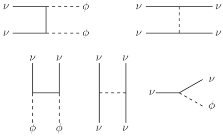
The $\phi$ boson can be brought into thermal equilibrium through its coupling to the neutrinos, and the $\nu-\phi$ system may stay in thermal contact until late times. The processes involved, shown in Figure 1, are $\nu\phi\leftrightarrow\nu\phi$, $\nu\nu\leftrightarrow\phi\phi$, $\nu\nu\leftrightarrow\nu\nu$, and either $\nu\leftrightarrow\nu\phi$ or $\nu\nu\leftrightarrow\phi$, depending on whether the scalar mass, $m_{\phi}$, is smaller or larger than the neutrino mass, $m_{\nu}$. For sufficiently large couplings, the $\nu$–$\phi$ system will remain in thermal contact until the temperature drops below $m_{\nu}$ or $m_{\phi}$. At this point the heavier of the two particles will annihilate or decay.

The possibility of altering the relativistic energy density through neutrino decay has been considered in CosmoDecay , while the cosmological effects of neutrino annihilation or self-interaction were examined in raffelt ; CosmoAnnil . In particular, raffelt considered the introduction of self-interactions as a mechanism to eliminate neutrino free-streaming, thus obtaining neutrinos which behave as cold dark matter, despite their light mass. However, in these scenarios the neutrinos were taken to be heavy enough ($m_{\nu}\sim 10{\rm eV}$) to contribute all of the dark matter, which is no longer a viable possibility. As we will show below, the combined use of neutrino mass limits and cosmological observations now allow much more sensitive constraints to be placed on these types of models.

The ultimate effect of the interaction shown in Eq. (1) can be split into two distinct cases, depending on whether the scalar is lighter or heaver than the neutrinos. We now discuss these cases in turn.

II.1 Light Scalars, $m_{\phi}<m_{\nu}$

When $m_{\phi}<m_{\nu}$, the neutrinos can annihilate to scalars via the process $\nu\nu\rightarrow\phi\phi$ when the temperature drops below $m_{\nu}$. Complete annihilation occurs provided that $g\gtrsim 10^{-5}$, although smaller couplings would suffice to keep the $\nu$–$\phi$ system in thermal equilibrium until late times via decay/inverse decay processes. Obtaining partial annihilation (rather than either negligible annihilation or complete annihilation) would require fine-tuning of $g$.

If all three neutrino species completely annihilate, they will make no contribution to the dark matter density in the universe today, as we would be left with a “neutrinoless universe” at late times. This eliminates cosmological constraints on neutrino mass neutrinoless . However, a nonzero $\phi$ mass would make a small contribution to the dark matter density. Note that $m_{\phi}<m_{\nu}$ implies the neutrinos are unstable, and may decay via $\nu_{i}\rightarrow\nu_{j}\phi$. For the same range of couplings, $g\gtrsim 10^{-5}$, this could lead to neutrino decay over astronomical distances, which is testable in future neutrino telescope experiments decay .

II.2 Light Neutrinos, $m_{\phi}>m_{\nu}$

Alternatively, if $m_{\phi}>m_{\nu}$, the scalar will eventually convert to neutrinos, so that cosmological neutrino mass bounds do apply. For example, the decay/inverse-decay process $\phi\leftrightarrow\nu\nu$, will keep the $\nu-\phi$ system tightly coupled throughout the CMB era, provided $g\gtrsim 10^{-12}$ chacko . Once the inverse process becomes kinematically inaccessible at $T\sim m_{\phi}$, the $\phi$ bosons will decay to neutrinos.

III Tightly coupled perturbation equations

For most parameters of interest, the neutrino mean free path is much smaller than the scales of interest during the epoch of CMB decoupling. In this limit, the neutrinos and bosons form a single, tightly coupled fluid. Perturbations in this fluid evolve differently, compared to the usual collisionless neutrino background. As they are coupled via gravity, neutrino perturbations influence the evolution of photon perturbations and thus neutrino perturbations can leave a distinctive signature in the CMB. In this section we discuss the relevant properties of the $\nu$–$\phi$ fluid for interesting limits of the model considered in Section II and in a more general context.

In the standard scenario, free-streaming damps the neutrino density perturbations, and introduces a source of anisotropic stress, e.g. see hu ; bashinsky . In comparison, a tightly-coupled fluid has only density and velocity perturbations, with the shear stresses and all higher moments in the Boltzmann hierarchy absent (at least to linear order). Defining the density and velocity perturbations as $\delta=\delta\rho/\rho$ and $\theta=ikv$ respectively, the equations describing the evolution of the tightly-coupled $\nu$–$\phi$ fluid are

$$\dot{\delta} = -(1+\omega)\left(\theta+\frac{\dot{h}}{2}\right)-3\frac{\dot{a}}{a}\left(c_{s}^{2}-\omega\right)\delta,$$ (2)

$$\dot{\theta} = -\frac{\dot{a}}{a}\left(1-3\omega\right)\theta-\frac{\dot{\omega}}{1+\omega}\theta+\frac{c_{s}^{2}}{1+\omega}k^{2}\delta,$$ (3)

in the synchronous gauge, where an overdot is a derivative with respect to conformal time. Here, $c_{s}^{2}=\delta P/\delta\rho$ is the adiabatic sound speed and $\omega=P/\rho$ is the equation of state with $\rho=\rho_{\nu}+\rho_{\phi}$ and $P=P_{\nu}+P_{\phi}$. In the limit where both $\nu$ and $\phi$ are relativistic $\omega=c_{s}^{2}=1/3$. However, for non-zero masses, $\omega$ and $c_{s}^{2}$ temporarily decrease from $1/3$ and deviate from each other, during the period when $\nu$ or $\phi$ starts to become non-relativistic and annihilate/decay. We may define an effective number of standard model neutrinos $N^{\rm int}_{\nu}$ contributed by the $\nu$–$\phi$ fluid with the relation

$$\rho=N^{\rm int}_{\nu}\frac{7}{8}\frac{\pi^{2}}{15}\left(T_{\nu}^{\mbox{\tiny SM}}\right)^{4},\,$$ (4)

where $T^{\rm SM}_{\nu}=(4/11)^{1/3}T_{\gamma}$ is the canonical cosmic neutrino background temperature in the standard model. The value of $N^{\rm int}_{\nu}$ after the heavier species annihilates into the lighter will be greater than the value before annihilation. Details of the calculation of $w$, $c_{s}^{2}$, and $N^{\rm int}_{\nu}$ can be found in Appendix A.

The differences from standard cosmology in these models will therefore typically be a combination of (i) elimination of neutrino free-streaming, (ii) nonstandard equation of state and sound speed evolution, and (iii) additional (and perhaps an evolving amount of) relativistic energy density. We now consider two phenomenological models (limiting cases of the interaction model of Section II) that exhibit these differences.

III.1 Model A: Freestreaming vs. Interacting (Massless Particles)

In this section we consider a scenario in which some fraction of the neutrinos act as a tightly-coupled fluid, but where $N^{\rm eff}_{\nu}$ is constant with time. We parameterize this class of models by $N^{\rm SM}_{\nu}$ and $N^{\rm int}_{\nu}$, the number of standard model (free-streaming) and interacting degrees of freedom respectively, where

$$N^{\rm eff}_{\nu}=N^{\rm SM}_{\nu}+N^{\rm int}_{\nu}.$$ (5)

A scenario in which $N^{\rm eff}_{\nu}$ is constant in time corresponds, for example, to the limit $m_{\nu}\rightarrow 0$ and $m_{\phi}\rightarrow 0$. However, even for finite masses, this limit is a good approximation as long as $N^{\rm eff}_{\nu}$ does not evolve significantly during the times of interest, as would be the case if any annihilation/decay takes place well before or well after the CMB decoupling epoch. In particular, this is a reasonable approximation for the $m_{\phi}>m_{\nu}$ models considered in chacko , where only modest evolution of $N^{\rm eff}_{\nu}$ occurs.

Note that this description is much more general than any particular limit of a neutrino-scalar interaction model. It encompasses any scenario in which some fraction of the energy density is in free-streaming relativistic particles, and another fraction is in a tightly-coupled relativistic fluid, as long as $N^{\rm eff}_{\nu}$ does not evolve significantly.

Figure 2: CMB and matter power spectra as a function of the fraction of interacting neutrinos, with $N^{\rm eff}_{\nu}\equiv N^{\rm SM}_{\nu}+N^{\rm int}_{\nu}=3$. The power spectra are normalized (to an arbitrary value) at large scale.

Figure 3: Upper: The CMB power spectra due to the monopole, velocity, and ISW terms of the source function for the standard $N^{\rm int}_{\nu}=0$ case (For a pedagogical description of these terms see, e.g., Refs. Seljak:1996is ; Dodelson:2003ft ). Lower: The contribution of each source term to $\Delta C_{l}$, the difference between a model with $N^{\rm int}_{\nu}=3$ and $N^{\rm int}_{\nu}=0$ with $N^{\rm eff}_{\nu}=3$ held fixed. The ISW-monopole cross term (nonzero due to the differing evolution of the gravitational potentials) contributes significantly to the difference in the first peak despite the identical background evolution of the two models.

Figure 4: The CMB and matter power spectra as a function of the number of standard model neutrinos, with $N^{\rm int}_{\nu}=0$. The power spectra are normalized (to an arbitrary value) at large scale.

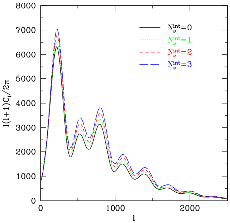
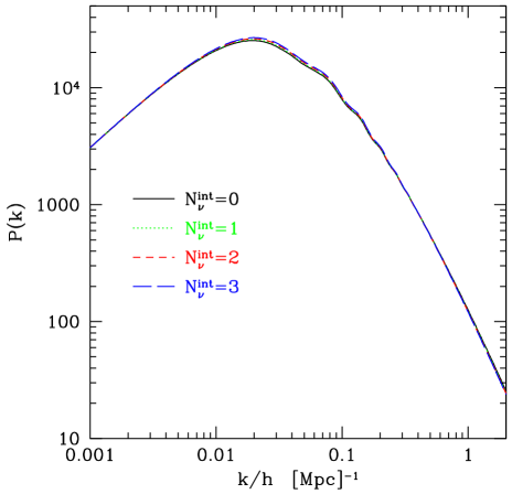
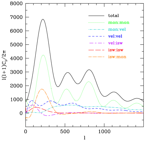
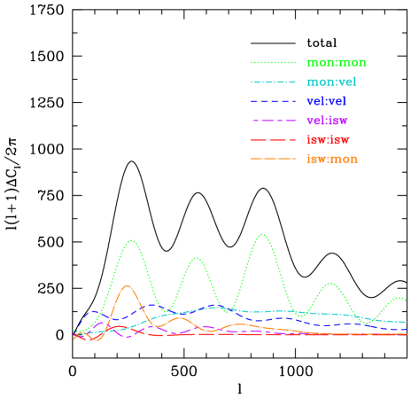
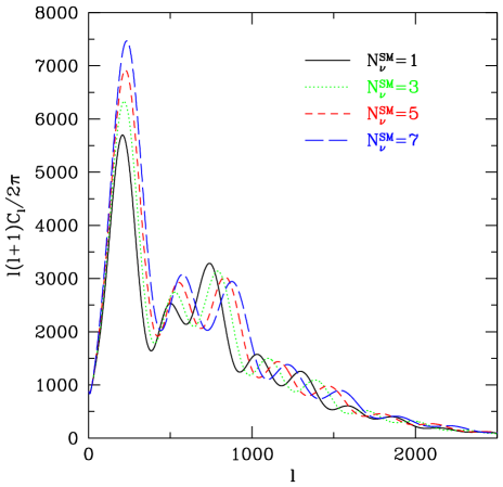
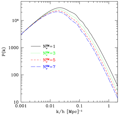
Fig. 2 shows effects on the CMB angular power spectrum and the matter power spectrum of varying the number of interacting neutrinos, while $N^{\rm eff}_{\nu}$ and all other cosmological parameters are held fixed. This allows us to explore the effects of suppressed neutrino free streaming alone. In the standard case ($N^{\rm int}_{\nu}=0$) when a perturbation of a given scale enters the horizon, power is transfered from the neutrino density modes to higher moments of the neutrino distribution as the neutrinos free-stream out of gravitational potentials. This effect does not occur for interacting neutrinos which instead contribute to the gravitational potential and thus enhance the monopole perturbation of the photon distribution and increase the amplitude of the CMB temperature power spectrum for a fixed amplitude of primordial perturbations. Indeed, we see that beyond the first peak the effect of increasing $N^{\rm int}_{\nu}$ in the CMB can be roughly approximated as a constant offset in the amplitude of the spectrum. A small shift in the location of the peaks is also a feature bashinsky . In the upper panel of Fig. 3 we show the contributions to the CMB power spectrum arising from the monopole terms (the physical temperature perturbation at the last-scattering surface corrected for its gravitational redshift), the velocity terms (perturbations due to the Doppler shift), and the ISW terms (perturbations due to the evolving gravitational potentials) of the source function (see, for example, Refs. Seljak:1996is ; Dodelson:2003ft for a pedagogical review of the source function). The lower panel of Fig. 3 shows the difference in CMB power spectra between models with $N^{\rm int}_{\nu}=3$ and $N^{\rm int}_{\nu}=0$ keeping $N^{\rm eff}_{\nu}=3$ fixed (the extreme models of Fig. 2). While the change in the monopole dominates the total difference in the power spectrum at all $l$, the ISW-monopole cross term contributes significantly to the difference near the first peak. Note that this ISW-monopole contribution is nonzero solely because gravitational potentials evolve differently in a model with and without free-streaming neutrinos — the background evolution is identical in the two cases.

As we are in the limit of massless neutrinos, the effect on the matter power spectrum of suppressing free streaming is very minor. Free-streaming has a significant effect on the matter power spectrum when $m_{\nu}$ is finite, such that neutrinos contribute some fraction of the dark matter density today. In that case, the free-streaming of the neutrino hot dark matter component damps the growth of structure while the neutrinos are still relativistic. By comparison, the effect of modifications to the neutrino perturbations of massless neutrinos is very small.

For comparison, we show in Fig. 4 the effects on the CMB angular power spectrum and the matter power spectrum of varying the total relativistic energy density, $N^{\rm SM}_{\nu}$, while $N^{\rm int}_{\nu}$ and all other cosmological parameters are held fixed. We see that increasing $N^{\rm eff}_{\nu}$ enhances the first peak. This is the result of a larger ISW effect, due to the delay in matter-radiation equivalence. There is also a large shift in the positions of the subsequent peaks, which occurs due to the change in the conformal time of last scattering. See Ref. Pierpaoli for a discussion of these effects. In Fig. 4, we also see that the enhanced radiation density suppresses the matter power spectrum. Again, this is because matter-radiation equivalence, and hence the growth of structure, is delayed.

The extent to which the various effects discussed above can be compensated with a change in other cosmological parameters will be discussed in section V.

III.2 Model B: Neutrino Annihilation to Scalars

We now turn to the slightly more complicated scenario with $m_{\phi}<m_{\nu}$, where the interacting neutrinos can annihilate. We again assume the limit $m_{\phi}\rightarrow 0$, but allow a nonzero $m_{\nu}$. We specialize to the case of three neutrino species, and will consider the possibility that either one, two, or all three neutrino species interact strongly with the scalar $\phi$, which we shall denote by models B1, B2, and B3 respectively. For couplings constants $g\gtrsim 10^{-5}$, the neutrino species which are coupled to the scalar will annihilate when $T_{\nu}\sim m_{\nu}$. If all three neutrino species annihilate (model B3) this leaves a “neutrinoless universe”. Cosmological neutrino mass bounds are altered in these scenarios, because the neutrino species which annihilate will not make a contribution to the dark mater density today (i.e., they will not contribute to $\Omega_{\nu}$) neutrinoless .

Figure 5: The evolution of the effective number of interacting neutrinos $N^{\rm int}_{\nu}$ with $m_{\nu}=0.1$ eV (dashed curves), $m_{\nu}=1$ eV (dotted curves) and $m_{\nu}=10$ eV (solid curves) for 3 interacting neutrinos (top/red), 2 interacting neutrinos (middle/green), and 1 interacting neutrino (bottom/blue). Notice that the $N^{\rm int}_{\nu}$ initially includes an extra $4/7$ to account for the new scalar degree of freedom and that the effective number of interacting neutrinos after annihilation is greater than prior to annihilation.

Figure 6: The evolution of $w$, the equation of state (solid curves) and $c_{s}^{2}$, the sound speed (dotted curves) as a function of the scale factor, $a$, for $m_{\nu}=1$ eV for 3 interacting neutrinos (bottom/red), 2 interacting neutrinos (middle/green), and 1 interacting neutrino (top/blue). Both deviate from the value of $1/3$ for a relativistic fluid, during the epoch of annihilation.

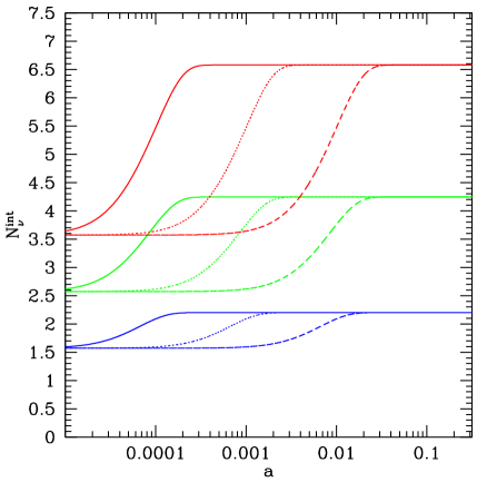
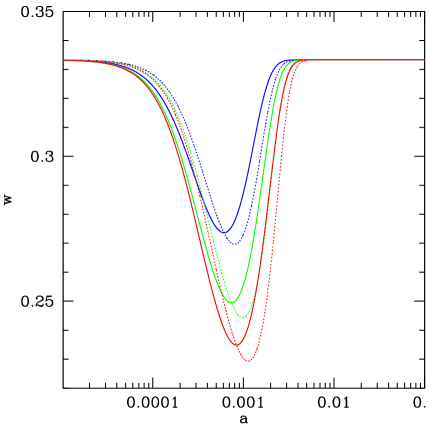
A distinctive feature of this scenario is that the neutrino annihilation will heat the scalars, causing $N^{\rm eff}_{\nu}$ to evolve as the annihilation proceeds. For simplicity, we shall assume the scalar boson is brought into thermal equilibrium before the neutrinos thermally decouple from the electrons and positrons (at $T\sim 1$ MeV). The scalar will then initially contribute an amount $\delta N_{\nu}=4/7$ to the relativistic energy density, so that $N^{\rm eff}_{\nu}\simeq 3.57$ . This value will increase as the annihilation proceeds. For example, if all three neutrinos annihilate, the final relativistic energy density is equivalent to $N_{\nu}\simeq 6.6$ neutrinoless (see also Appendix A). For realistic neutrino masses, $m_{\nu}\simeq 0-2$ eV, this annihilation occurs close to the time at which the CMB photons last scatter, so that the evolution of $N^{\rm eff}_{\nu}$ takes place during the CMB decoupling era. The evolution of $N^{\rm eff}_{\nu}$ is shown in Fig. 5. The evolution of the equation of state, $w$, and sound speed, $c_{s}^{2}$, during this annihilation epoch is shown in Figure. 6.

The present laboratory limit on neutrino mass is $m_{\nu}<2.2{\rm~{}eV}$, set by tritium beta decay experiments tritium . Given the tiny mass squared differences measured by solar and atmospheric neutrino oscillation experiments ($\delta m^{2}_{\rm sol}\simeq 7\times 10^{-5}{\rm~{}eV}^{2}$ and $\delta m^{2}_{\rm atm}\simeq 2\times 10^{-3}{\rm~{}eV}^{2}$ oscillation ), the tritium bound applies to all three neutrino mass eigenstates. We shall assume that the three neutrino eigenstates have degenerate masses, which is a good approximation for $m_{\nu}\gtrsim 0.1{\rm~{}eV}$. (We use $m_{\nu}$ to denote the value of a single neutrino mass throughout, so that the quantity $\Sigma m_{\nu}=3m_{\nu}$.) In the analysis in section V, we consider neutrino masses in the allowed range $m_{\nu}=0-2.2{\rm~{}eV}$.

For simplicity, we also assume that the scalar has sufficiently strong self-interactions that it continues to behave as a tightly-coupled fluid once the neutrino annihilation is complete. For early neutrino annihilation (large masses) this will result in the largest deviations of the CMB spectra with respect to the standard scenario. For late annihilation (small masses) the late-time behavior of the scalar is irrelevant.

Figure 7: The CMB and matter power spectra, for varying values of $m_{\nu}$, for model B1 (one interacting neutrino and two standard neutrinos). The power spectra are normalized (to an arbitrary value) at large scale.

Figure 8: The CMB and matter power spectra, for varying values of $m_{\nu}$, for model B3 (three interacting/annihilating neutrinos). The power spectra are normalized (to an arbitrary value) at large scale.

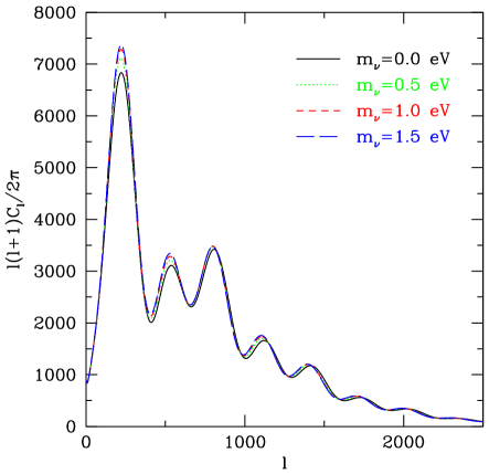
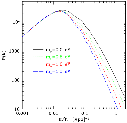
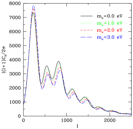
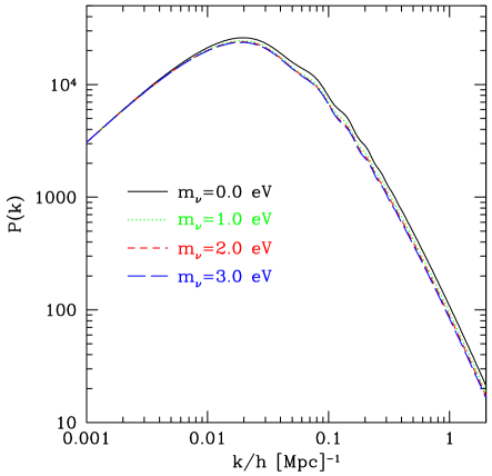
Fig. 7 shows effects on the CMB angular power spectrum and matter power spectrum of varying $m_{\nu}$ in the model with one interacting neutrino (B1), while Fig. 8 shows the same effects for the model with three interacting neutrinos (B3). Here we see a combination of the effects of free-streaming suppression (compare Fig 2) and larger $N^{\rm eff}_{\nu}$ (compare Fig. 4). In the CMB spectra, we see the enhanced overall amplitude which is characteristic of the tightly coupled neutrinos, together with an enhanced first peak and shifted subsequent peaks that result from increased relativistic energy density. As expected, the effects on the CMB spectra are more pronounced in model B3, in which all three neutrinos species annihilate. Moreover, the effect increases as $m_{\nu}$ increases, because larger mass corresponds to earlier annihilation, so that the extra relativistic energy density is present earlier.

Conversely, the effects on the matter power spectra are more pronounced in model B1 in which only one neutrino species annihilates. This is expected, because the remaining neutrinos contribute to the dark matter density today. This remaining neutrino hot dark matter component causes the usual suppression of the power spectrum that is used to constrain neutrino mass. However, in the “neutrinoless” model (B3), this suppression of the power spectrum is absent, because no neutrino dark matter component remains. A smaller power spectrum suppression does remain, as shown in Fig. 8. This small effect is a result of enhanced $N^{\rm eff}_{\nu}$, which slightly delays matter-radiation equivalence and hence delays the growth of structure. Again, this effect is more significant for larger $m_{\nu}$, because the extra radiation is present earlier. We thus see that the “neutrinoless universe” model (B3) can accommodate large neutrino mass, while having little effect on the matter power spectrum neutrinoless .

IV Data

We computed the CMB and large scale structure power spectra, and performed the parameter estimation with a modified version of the publicly available Markov Chain Monte Carlo package, COSMOMC COSMOMC ; CAMB .

Constraints on the models were evaluated using CMB data from the WMAP WMAP , ACBAR ACBAR and CBI CBI experiments, together with the galaxy power spectra measured by the 2dF Galaxy Redshift Survey 2dF and the Sloan Digital Sky Survey (SDSS) SDSS . In addition, we used the measurement of the Hubble parameter made by the Hubble Space Telescope (HST) Key Project HST . This set of data constitutes our basic comparison set (hereafter Cosmo). For model B3, we imposed a cut-off of 2.2 eV for the neutrino mass, consistent with the tritium beta decay limit tritium .

In addition, we will investigate how the introduction of the Lyman-$\alpha$ constraints lyman and the CMB polarization as measured by CBI CBIpol constrain these models. These two variants will be named CosmoLy$\alpha$ and CosmoCBIpol respectively. We implement the Lyman-$\alpha$ constraints derived in Ref. VHS04 and we implement them in a similar way as in Ref. lyman , with minor modifications that were suggested by the authors.

Note that SDSS and 2dF data impose a constraint only on the shape of the power spectrum, $P(k)$, and not on the normalization, as we make no assumptions about the bias. Lyman-$\alpha$ data, however, imposes constraints on both normalization and shape at small scales.

V Results

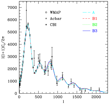
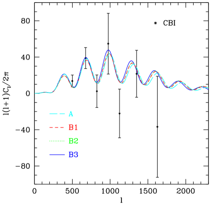
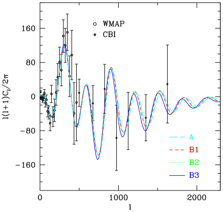
We now discuss how the different models fit the data. We first note that for all of the models, parameters sets can be found which provide a good global fit to the data, and so none of the models can be ruled out. For example, in Table 1 we report the $\chi^{2}$ values of the best fit points in our Markov chains for the case of the Cosmo data set. The table shows that the best fit parameter set for all the models considered indeed provides a good fit to the data. We plot spectra for the best fit models in Fig. 9. Apart from the high value of $N^{\rm SM}_{\nu}$ in model A (see the discussion at the end of the the next section), the best-fit parameters are within commonly adopted parameter ranges in the standard $\Lambda$CDM model.

Figure 9: The CMB temperature (TT, upper left), polarization (EE, upper right) and cross (TE, lower left) power spectra, and the matter power spectrum (lower right), for the best-fit models. In each case models can be found that fit all data well.

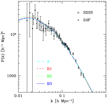
Model	$\chi^{2}$	DOF	Reduced $\chi^{2}$	$({\rm DOF}/2)^{-1/2}$
A	1515.00	1478	1.025	0.037
B1	1520.17	1479	1.028	0.037
B2	1523.99	1479	1.030	0.037
B3	1526.77	1479	1.032	0.037

Table 1: The $\chi^{2}$ values and degrees of freedom (DOF), using the Cosmo data set.

On the other hand, while reasonable parameters can be found that yield a good global fit to the data for each of model A, B1, B2, and B3, we will show that models with fewer interacting neutrinos are preferred in a Bayesian sense after marginalizing over all other cosmological parameters. The interpretation of these results is discussed further below. We shall now discuss each model individually, focusing on the constraints on the neutrino properties.

V.1 Model A: $N^{\rm SM}_{\nu}$ vs. $N^{\rm int}_{\nu}$

Fig. 10 displays the curves for the marginalized likelihood of the parameters $N^{\rm SM}_{\nu}$ and $N^{\rm int}_{\nu}$. Notice that the CMB alone allows a larger number of interacting neutrinos, while preferring a relatively low number of standard neutrinos. The addition of the matter power spectra yields the effect of reducing the maximum value of $N^{\rm int}_{\nu}$, and also shifts the peak of the likelihood for $N^{\rm SM}_{\nu}$. Referring to Fig. 2, we notice that keeping the total number of neutrinos fixed while increasing the number of interacting neutrinos has a large impact on the CMB power spectrum, and a very minor one on the matter power spectrum (the two models have equal total energy density, but different neutrino fluctuation evolution). However, the introduction of the matter power spectrum constraint in the likelihood analysis imposes limits on the epoch of equivalence, and on the total spectral index. This, in turn, leaves less freedom for accommodating non–standard neutrino fluctuation evolution which affects the CMB power spectrum.

Figure 10: The marginalized likelihood curves for $N^{\rm int}_{\nu}$ and $N^{\rm SM}_{\nu}$ in Model A. The solid curves corresponds to the Cosmo data set (CMB+2dF+SdDS+HST) and the long-dashed curve to the CMB data alone. The dotted and short-dashed curves correspond to the addition of the Lyman-$\alpha$ and CBI polarization data respectively.

As anticipated in Pierpaoli , the addition of the Lyman–$\alpha$ constraint improves the limits on the standard model neutrinos. This is because by probing the power of the fluctuations on very small scales, the Lyman–$\alpha$ data places a strong constraint on the spectral index $n$ lyman , which is degenerate with $N^{\rm SM}_{\nu}$ and the reionization $\tau$ in the radiation power spectrum.

It is interesting to note that adding the CBI polarization data also improves the constraints on $N^{\rm SM}_{\nu}$. This is because an increased number of neutrinos significantly shifts the peaks of the $C_{l}$, due to the delay in matter-radiation equivalence. The CBI polarization data have been shown to be able to determine the phase of the oscillations with high precision CBIpol , despite the size of the errorbars. This is one example of how such information can be used in constraining parameters.

Table 2 summarizes the best fit values and the 95 % confidence levels for the marginalized likelihoods for $N^{\rm SM}_{\nu}$ and $N^{\rm int}_{\nu}$, while Fig. 11 shows the degeneracy between $N^{\rm SM}_{\nu}$ and $N^{\rm int}_{\nu}$ in the case of the Cosmo dataset. A higher value for $N^{\rm int}_{\nu}$ may be compensated by a lower value for $N^{\rm SM}_{\nu}$. However, once the matter power spectrum is used in the analysis (and thus the redshift of equivalence is constrained) the degeneracy is mild.

	$N^{\rm SM}_{\nu}$	$N^{\rm SM}_{\nu}$	$N^{\rm int}_{\nu}$	$N^{\rm int}_{\nu}$
Data set	best fit	upper limit	best fit	upper limit
Cosmo	5.0	7.8	0.015	2.9
CosmoCBIpol	4.3	6.9	0.1	2.9
CosmoLy$\alpha$	4.9	6.8	0.02	3.0

Table 2: The best fit values and 95 % C.L. allowed ranges for $N^{\rm SM}_{\nu}$ and $N^{\rm int}_{\nu}$ in Model A. The confidence limits are obtained from marginalized curves.

Figure 11: Upper: The contour level for the parameters $N_{\nu}^{\rm SM}$ and $N_{\nu}^{\rm int}$ in Model A. The two solid lines are one and two $\sigma$ contours, shades are from the mean likelihood, using the Cosmo data set. Lower: The relative likelihood along the line $N_{\nu}^{int}+N_{\nu}^{\rm SM}=3$.

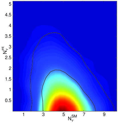
It is clear from Figs. 10 and 11 that models with fewer than three interacting neutrinos are favored in a Bayesian sense. This does not contradict our previous statement that cosmological parameter values can be found with $N^{\rm int}_{\nu}\simeq 3$ which provide a good global fit to the data considered (a reduced $\chi^{2}$ statistically consistent with 1). It is worth elaborating on the implications and interpretation of this Bayesian limit and why no contradiction exists. Firstly, the likelihoods shown are after marginalizing over all other parameters assuming flat priors in $N^{\rm SM}_{\nu}$, $N^{\rm int}_{\nu}$, and all other cosmological parameters. As such, the likelihood in Fig. 11 is not straightforward measure of the goodness-of-fit of models with given values of $(N^{\rm SM}_{\nu},N^{\rm int}_{\nu})$ but also of the density of good-fitting models with the values $(N^{\rm SM}_{\nu},N^{\rm int}_{\nu})$ in the hyperplane of parameter space defined by the remaining cosmological parameters — it technically quantifies the cumulative relative likelihood of two populations of models. We can certainly conclude, for instance, from Fig. 11 that (with the aforementioned flat priors) the set of data we have used prefers the population of models with $(N^{\rm SM}_{\nu},N^{\rm int}_{\nu})\simeq(3,0)$ relative to the population of models with $(N^{\rm SM}_{\nu},N^{\rm int}_{\nu})\simeq(0,3)$ at more than 2-$\sigma$. However, we can not conclude from Fig. 11 that all models with $(N^{\rm SM}_{\nu},N^{\rm int}_{\nu})\simeq(0,3)$ are ruled out at more than 2-$\sigma$ by current data. This conclusion can only be made if no models with $(N^{\rm SM}_{\nu},N^{\rm int}_{\nu})\simeq(0,3)$ can be shown to be consistent with the data, which as we have discussed, is not the case. Similarly, while we can conclude that the population of models with $(N^{\rm SM}_{\nu},N^{\rm int}_{\nu})\simeq(3,0)$ are disfavored compared to the population of models with $(N^{\rm SM}_{\nu},N^{\rm int}_{\nu})\simeq(5,0)$ we can not conclude that all models with $5$ free-streaming neutrinos provide better global fit to the data than all models with $3$ free-streaming neutrinos. This is just the nature of Bayesian inference — it attempts to quantify the relative likelihood of models within a given paradigm, but does not make an absolute judgment on the viability of the paradigm itself (or in this case a particular subset of the models within the paradigm). To make a judgment on the viability of a given paradigm, a better approach is to ask the question “Are there any models within this paradigm which are consistent with the data?”. If the answer to this question is “yes” then that paradigm is still viable. In this case, another way of summarizing the state of affairs is that even if priors stipulating $(N^{\rm SM}_{\nu},N^{\rm int}_{\nu})\simeq(3,0)$ or $(N^{\rm SM}_{\nu},N^{\rm int}_{\nu})\simeq(0,3)$ are imposed to restrict our paradigm to either the standard model of particle physics or an alternative model with interacting neutrinos, then models that are globally consistent with the data can still be found (albeit fewer of them in the later case).

Finally, let us comment on parameter degeneracy. Because the number of neutrinos contribute to setting the redshift of equivalence, both $N^{\rm SM}_{\nu}$ and $N^{\rm int}_{\nu}$ are degenerate with $\Omega_{m}$ and $H_{0}$. It has been pointed out Pierpaoli ; Nnu that a higher number of massless neutrinos can be compensated by a higher $H_{0}$. We find that even the marginalized likelihood for $H_{0}$ in this model is around 80 ${\rm km}\ {\rm s}^{-1}\ {\rm Mpc}^{-1}$, which is only one $\sigma$ away from the HST quoted best fit. In this respect, our results are discrepant with those in hannestad , where much larger values of $H_{0}$ were obtained.

V.2 Model B: Annihilating neutrinos

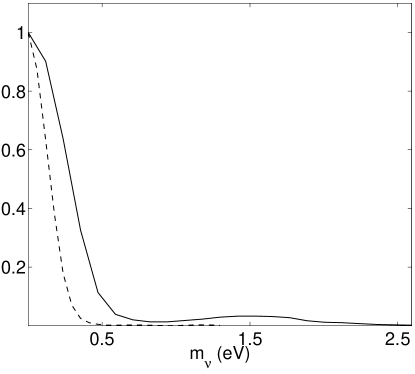
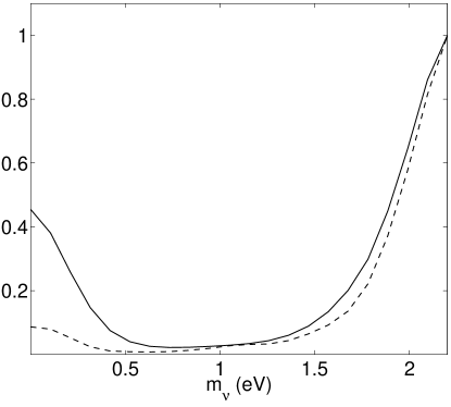
In Fig. 12 we plot the marginalized likelihood for the neutrino mass in model B1 (one interacting neutrino plus 2 standard model neutrinos) using the Cosmo and Cosmo + Lyman–$\alpha$ data sets (CosmoLy$\alpha$). The curves for B2 are similar to B1. In Fig 13, we show the corresponding likelihood for the case where all three neutrinos annihilate (model B3). The best fit values and the 95 % C.L. of the marginalized likelihoods are reported in table 3, for the model in which either one, two or three neutrinos interact and annihilate. For models B1 and B2 the best fits are at $m_{\nu}\simeq 0~{}\rm{eV}$. Note that our approximation does not allow us to explore $m_{\nu}\simeq 0~{}\rm{eV}$, as the assumption that all three neutrino masses are equal breaks down when $m_{\nu}\lesssim\sqrt{\delta m^{2}_{\rm atm}}\sim 0.05~{}\rm{eV}$. For model B3 the best fit is non-zero, and is discussed further below.

Figure 12: Marginalized likelihood for the neutrino mass in Model B1. The solid curve and dashed curves correspond to the Cosmo and CosmoLy$\alpha$ data sets respectively.

Figure 13: Marginalized likelihood for the neutrino mass in the “neutrinoless universe” model, B3. The solid and dashed curves correspond to the Cosmo and CosmoLy$\alpha$ data sets respectively. Note that we imposed a 2.2 eV cut-off for $m_{\nu}$.

	B1	B1	B2	B2	B3	B3
Data set	best fit	limit	best fit	limit	best fit	limit
Cosmo	$<0.1$	1.5	$<0.1$	0.42	2.2	2.2
CosmoLy$\alpha$	$<0.1$	0.24	$<0.1$	0.31	2.2	2.2

Table 3: The limits on the neutrino mass, in the various models. All values are in eV. For each model, the upper limit refers to the 95 % C.L. limit of the marginalized likelihood. For $m_{\nu}<0.1$ eV, the approximation that all three neutrino masses are degenerate is not satisfied. Note that for model B3, we imposed a 2.2 eV cut-off, as implied by the tritium beta decay neutrino mass limit.

For the cases B1 and B2 where only one or two neutrino species annihilate, the remaining neutrinos contribute to the dark matter density today. As expected, Lyman-$\alpha$ data significantly tightens the neutrino mass limit in these models, because it sets a constraint on the overall normalization and the shape of the power spectrum. This reduces the 95 % C.L. upper limit by quite a lot, bringing it to 0.24 eV for one interactive neutrino (model B1) and 0.31 eV for 2 interactive neutrinos (model B2). The addition of the CBI polarization data does not improve the constraints on neutrinos mass with respect to those obtained with the Cosmo data. This is because such low neutrino masses don’t have a significant impact on the CMB power spectrum (see Fig. 7). As for degeneracies, the neutrino mass parameter is degenerate with $\Omega_{m}$ and $\Omega_{\Lambda}$ and $H_{0}$, all of which affect the redshift of equivalence and therefore the amplitude of the matter power spectrum at small scales. As a consequence, $m_{\nu}$ is also degenerate with the amplitude of the matter power spectrum $\sigma_{8}$. The mean of the marginalized $H_{0}$ likelihood plot is 68 ${\rm km}\ {\rm s}^{-1}\ {\rm Mpc}^{-1}$ and 71 ${\rm km}\ {\rm s}^{-1}\ {\rm Mpc}^{-1}$ for models B1 and B2, which are perfectly normal values.

The case B3 is different, because here all three neutrinos species annihilate, leaving no neutrino contribution to the dark matter today. The effects on the power spectrum are thus milder (see Fig. 8), and hence the limits on the neutrino mass are expected to be significantly weaker. In particular, the more massive the neutrino is, the earlier it annihilates (see Fig. 5). If the neutrinos annihilate early enough that all cosmologically interesting scales are outside the horizon, then models corresponding to different masses only differ by a slightly different expansion history very early on. Therefore, the data cannot distinguish between different high values of $m_{\nu}$, as the corresponding power spectra are very similar (see Fig. 8 and Fig. 14.)

Figure 14: The confidence level contours for the parameters $\Omega_{b}h^{2}$, Age, $H_{0}$, and $\sigma_{8}$, vs. $m_{\nu}$, for model B3. The solid lines are the one and two sigma contours, and shades are from the mean likelihood, using the Cosmo data set. The panels on the left have a 2.2 eV cut-off imposed on $m_{\nu}$, while the panels on the right have a 15 eV cut-off.

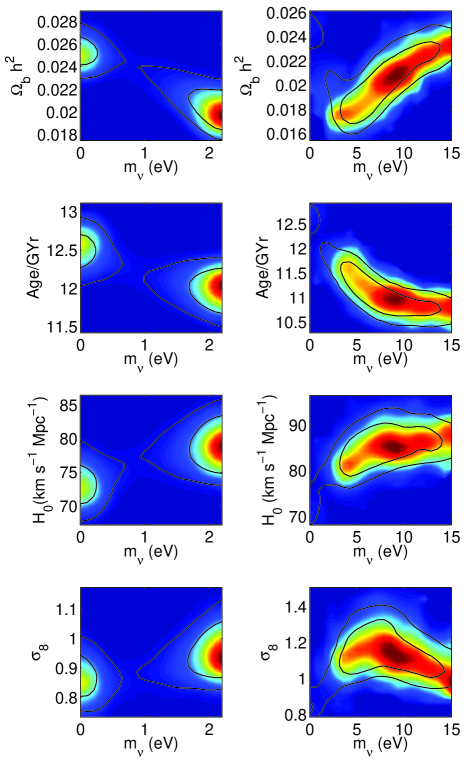
However, for neutrino masses $m_{\nu}\simeq 1$ eV, the annihilation takes place very close to the time of CMB decoupling. It is during the annihilation period that the greatest deviation of the sound speed and the equation of state occur (see Fig. 6.) Hence for $m_{\nu}\simeq 1$ eV, the CMB spectrum is affected by the modified values of $w$ and $c_{s}^{2}$, in addition, of course, to the lack of free-streaming. This tends to disfavor $m_{\nu}\simeq 1$ eV, with respect to both larger and smaller values of $m_{\nu}$, as shown in Fig. 13.

In addition, the neutrino mass in model B3 shows significant degeneracies with the Age and $H_{0}$, as changes in these parameters compensate for the effect of increased radiation density on the epoch of equivalence. The neutrino mass is also degenerate with $\Omega_{b}h^{2}$ and $\sigma_{8}$. We have plotted these degeneracies in Fig. 14. To help explore the degeneracies, we have determined the marginalized likelihood contours with and without imposing the 2.2 eV cut-off in $m_{\nu}$. We can see from Fig. 14 that although a slightly better fit is obtained for larger $m_{\nu}$ (5-10 eV), this would imply an unacceptably low Age Age , an unacceptably high $H_{0}$, and also a value of $\sigma_{8}\gtrsim 1$, which is disfavored by recent cluster number counts clusters and lensing analysis lensing . (The baryon abundance however, more closely matches the BBN determination, $\Omega_{b}h^{2}=0.022\pm 0.002$ BBN , for larger values of $m_{\nu}$.) Imposing the 2.2 eV cut-off for $m_{\nu}$ (as required to be consistent with the tritium beta decay neutrino mass limit) brings these parameters back to more reasonable values. However, even in the 0-2.2 eV region, the values of these parameters seem somewhat discrepant. For example, the best fit point (at $m_{\nu}$ = 2.2 eV) has values of $\Omega_{b}h^{2}$, Age and $H_{0}$ which all deviate from the central values preferred by BBN, globular cluster, and HST measurements, respectively, by about one sigma.

V.3 Discussion

The results above should be compared with the ones obtained by other authors in the standard case of three massive, non–interacting neutrinos. The WMAP team found $m_{\nu}\leq 0.23~{}{\rm eV}$ at 95 % CL Sper03 , using CMB data and the 2dF power spectrum, plus an assumption on the power spectrum bias which drives most of the result pierpaproc ; ElgLah . The addition of quite tight constraints from the SDSS power spectrum leads to an upper limit on the sum of the three masses of $\sum m_{\nu}=0.42~{}{\rm eV}$ at 95 % CL selj04 . The recent results from the Boomerang team are $m_{\nu}<1~{}{\rm eV}$ at 95 % CL from CMB data alone, and $m_{\nu}<0.4~{}{\rm eV}$ when the matter power spectrum data are considered, with no bias assumptions boom05 . Perhaps the most directly comparable value is the one obtained by vielproc , $\sum m_{\nu}=0.33\pm 0.27~{}{\rm eV}$, with the same Lyman–$\alpha$ sample and comparable assumptions about the parameters as in our analysis. These results are broadly similar to what we find for the cases B1 and B2, in which one or two standard model neutrinos remain. As a general result, we can conclude that the neutrino mass is expected to be below about 0.5 eV in those cases, and is not significantly affected by the presence of the tightly-coupled component of the relativistic energy density. However, the “neutrinoless” model (B3) is different, and leads to much weaker $m_{\nu}$ constraints, albeit at the expense of somewhat discrepant values for $\Omega_{b}h^{2}$, Age and $H_{0}$.

Finally, we comment on the implications of these results for neutrino decay. One consequence of strong $\nu-\phi$ interactions is that neutrinos may be unstable. For the range of couplings considered here, $g\gtrsim 10^{-5}$, the neutrinos could decay over astronomical distances, which is testable in neutrino telescope experiments decay . For small masses, the cosmological consequences of these couplings are represented by Model A, while for larger masses they are represented by either Model B2 or B3 (depending on whether one or two neutrino species are unstable.)

Ref. hannestadraffelt claims stringent limits on the couplings $g_{ij}$, and thus on neutrino lifetimes, based upon the fact that Refs. hannestad ; trotta find some evidence for neutrino free-streaming in the CMB. However, hannestad ; trotta analyzed only a scenario in which all three neutrinos behave in the same way, and thus certainly cannot be used to claim that all three neutrino species must be free-streaming.

Given the results here, we conclude that current cosmological data does not impose limits on either the individual couplings, $g_{ij}$, or upon neutrino lifetimes.

VI Conclusions

We have investigated the distinction between a free-streaming or interacting fluid of neutrinos, and explored the constraints on these neutrinos imposed by cosmology. Although some of our results are applicable in a wider context, we have used an example involving additional couplings between the neutrinos and a light boson. Our main conclusion is that models with interacting neutrinos remain viable, contrary to the claim in Ref.hannestad ; hannestadraffelt .

As a general result, we find that both CMB polarization data and Lyman–$\alpha$ data help to constrain the number of standard model neutrino species. The inclusion of Lyman–$\alpha$ data also helps improve the constraints on neutrino mass. With the data considered, we have found upper limits on the neutrino mass, but no detection of a nonzero neutrino mass.

Two parameterizations of the interacting-neutrino models have been examined:

(1) In the first, we allowed for an arbitrary number of free-streaming (standard model) neutrinos, $N^{\rm SM}_{\nu}$, and tightly-coupled (interacting) neutrinos, $N^{\rm int}_{\nu}$. Within the context of the neutrino-scalar model, this corresponds to the limit $m_{\nu}\rightarrow 0$ and $m_{\phi}\rightarrow 0$. We have found that within the ($N^{\rm SM}_{\nu}$,$N^{\rm int}_{\nu}$) plane, the data favors free-streaming neutrinos over tightly-coupled neutrinos in a Bayesian analysis. However, we find even if the prior $N^{\rm SM}_{\nu}\simeq 0$ is imposed (so that all neutrinos are interacting) models can be found that are a good global fit to the data considered, without resorting to extreme values for the cosmological parameters. In this respect, models with interacting neutrinos remain viable. We emphasize that the constraints obtained here are very general, as $N^{\rm SM}_{\nu}$ and $N^{\rm int}_{\nu}$ can parametrize any free-streaming or tightly coupled relativistic degrees of freedom, which need not consist of neutrinos.

(2) Our second parametrization consists of models with non-zero $m_{\nu}$. We fixed the total number of neutrinos to three, and allowed either one, two, or all three, to interact with a massless boson. In this scenario, the interacting neutrinos annihilate to bosons when $T\sim m_{\nu}$, thus removing them from the plasma. In the case where either one or two neutrino species interact/annihilate, we find the upper limits on neutrino mass are broadly similar to those for the standard scenario. However, if all three neutrino species annihilate to leave a “neutrinoless universe”, the neutrino mass limits are significantly weaker. In this case, values of $m_{\nu}$ comparable to the tritium beta decay limit of 2.2 eV are permitted, although a low Age and a high $H_{0}$ tend to somewhat disfavor the scenario.

Appendix A Neutrino-Scalar Fluid Properties

Here we summarize a few basic relationships for Fermi-Dirac and Bose-Einstein statistics and derive from them the quantities $w$, $c_{s}$, and $N^{\rm int}_{\nu}$ used in Eqs. (2)–(4) to evolve the perturbation dynamics and shown in Fig. 5 and Fig. 6. We note that these quantities may also be found by solving the continuity equations for energy and entropy density numerically, but we believe the analytical forms we present here are physically illustrative and may be useful in other contexts.

The number density $n_{i}$, energy density $\rho_{i}$, and pressure $P_{i}$ of a fermionic ($\xi=1$) or bosonic ($\xi=-1$) species $i$ of mass $m_{i}$ with $g_{i}$ internal degrees of freedom in thermal equilibrium can be written as

$$n_{i} =\frac{g_{i}}{2\pi^{2}}\int_{0}^{\infty}p^{2}dp\frac{1}{1+\xi e^{E/T}}$$

$$=\frac{g_{i}m_{i}^{3}}{2\pi^{2}}\sum_{n=1}^{\infty}\frac{(-\xi)^{\scriptscriptstyle n+1}}{{\rm n}x}\left[K_{2}({\rm n}x)\right]$$

$$\rightarrow g_{i}\left[\frac{3}{4}+\frac{1}{8}(1-\xi)\right]\frac{\zeta(3)}{\pi^{2}}T^{3}$$ (6)

$$\rho_{i} =\frac{g_{i}}{2\pi^{2}}\int_{0}^{\infty}p^{2}dp\frac{E}{1+\xi e^{E/T}}$$

$$=\frac{g_{i}m_{i}^{4}}{2\pi^{2}}\sum_{n=1}^{\infty}\frac{(-\xi)^{\scriptscriptstyle n+1}}{{\rm n}x}\left[K_{1}({\rm n}x)+\frac{3}{{\rm n}x}K_{2}({\rm n}x)\right]$$

$$\rightarrow g_{i}\left[\frac{7}{8}+\frac{1}{16}(1-\xi)\right]\frac{\pi^{2}}{30}T^{4}$$ (7)

$$P_{i} =\frac{g_{i}}{6\pi^{2}}\int_{0}^{\infty}p^{2}dp\frac{p^{2}/E}{1+\xi e^{E/T}}$$

$$=\frac{g_{i}m_{i}^{4}}{2\pi^{2}}\sum_{n=1}^{\infty}\frac{(-\xi)^{\scriptscriptstyle n+1}}{{\rm n}x}\left[\frac{1}{{\rm n}x}K_{2}({\rm n}x)\right]$$

$$\rightarrow g_{i}\left[\frac{7}{8}+\frac{1}{16}(1-\xi)\right]\frac{\pi^{2}}{90}T^{4}$$ (8)

where $E=\sqrt{p^{2}+m_{i}^{2}}$, $x\equiv m_{i}/T$, $K_{\alpha}$ are modified Bessel functions of the second kind, $\zeta(3)=1.2020569$ is the Riemann zeta function of three, and the arrows indicate the high-temperature limit $x\rightarrow 0$. Notice that the standard result for massless particles $P_{i}=\rho_{i}/3$ is recovered in this limit. These results can be straightforwardly derived by expanding the distribution function as a geometric series of Boltzmann factors. This form is useful for tabulating the density and pressure as the $K_{\alpha}$ can be rapidly evaluated and the sum converges quickly and can be truncated to the desired accuracy — keeping only the leading term is the Maxwell-Boltzmann approximation to the distribution function.

Specializing to the fermionic case ($\xi=1$) we write the energy density and pressure of a single fermionic degree of freedom as

$$\rho_{f} \equiv\frac{7}{8}\frac{\pi^{2}}{30}\chi_{\rho}(x)T^{4}$$

$$=\frac{m_{f}^{4}}{2\pi^{2}}\sum_{n=1}^{\infty}\frac{(-)^{\scriptscriptstyle n+1}}{{\rm n}x}\left[K_{1}({\rm n}x)+\frac{3}{{\rm n}x}K_{2}({\rm n}x)\right]$$ (9)

$$P_{f} \equiv\frac{7}{8}\frac{\pi^{2}}{90}\chi_{P}(x)T^{4}$$

$$=\frac{m_{f}^{4}}{2\pi^{2}}\sum_{n=1}^{\infty}\frac{(-)^{\scriptscriptstyle n+1}}{{\rm n}x}\left[\frac{1}{{\rm n}x}K_{2}({\rm n}x)\right]\,,$$ (10)

where $\chi_{\rho/P}\rightarrow 1$ for $x\rightarrow 0$ but are $<1$ for finite $x$. We also find it useful to define

$$\frac{d\rho_{f}}{dT} \equiv 4\cdot\frac{7}{8}\frac{\pi^{2}}{30}\chi_{d\rho}(x)T^{3}$$

$$=\frac{4}{T}\cdot\frac{m_{f}^{4}}{2\pi^{2}}\sum_{n=1}^{\infty}\frac{(-)^{{\scriptscriptstyle n+1}}}{{\rm n}x}\left[\frac{3}{4}K_{1}({\rm n}x)+\frac{12+{\rm n}x}{4{\rm n}x}K_{2}({\rm n}x)\right]$$ (11)

$$\frac{dP_{f}}{dT} \equiv 4\cdot\frac{7}{8}\frac{\pi^{2}}{90}\chi_{dP}(x)T^{3}$$

$$=\frac{4}{T}\cdot\frac{m_{f}^{4}}{2\pi^{2}}\sum_{n=1}^{\infty}\frac{(-)^{{\scriptscriptstyle n+1}}}{{\rm n}x}\left[\frac{1}{4}K_{1}({\rm n}x)+\frac{1}{{\rm n}x}K_{2}({\rm n}x)\right]\,,$$ (12)

where similarly $\chi_{d\rho/dP}\rightarrow 1$ for $x\rightarrow 0$.

Let us now consider, as we do in this paper, a thermalized fluid at temperature $T_{\nu\phi}$ consisting of $N$ massive neutrinos coupled to a single massless scalar degree of freedom $\phi$.

The total energy density and pressure of this fluid are

$$\rho=\rho_{\phi}+\rho_{\nu}=\frac{\pi^{2}}{30}T_{\nu\phi}^{4}+2N\frac{7}{8}\frac{\pi^{2}}{30}\chi_{\rho}(x_{\nu})T_{\nu\phi}^{4}$$ (13)

and

$$P=P_{\phi}+P_{\nu}=\frac{\pi^{2}}{90}T_{\nu\phi}^{4}+2N\frac{7}{8}\frac{\pi^{2}}{90}\chi_{P}(x_{\nu})T_{\nu\phi}^{4}$$ (14)

where the factor of $2$ in the neutrino terms accounts for anti-neutrinos and $x_{\nu}\equiv m_{\nu}/T_{\nu\phi}$.

We can now write the equation of state $w=P/\rho$ in terms of $\chi_{\rho}$ and $\chi_{P}$ as

$$w=\frac{1}{3}\left[\frac{4/7+N\chi_{P}(x_{\nu})}{4/7+N\chi_{\rho}(x_{\nu})}\right]\,.$$ (15)

Similarly, we can write the soundspeed $c_{s}^{2}=dP/d\rho$ in terms of $\chi_{d\rho}$ and $\chi_{dP}$ as

$$c_{s}^{2}=\frac{1}{3}\left[\frac{4/7+N\chi_{dP}(x_{\nu})}{4/7+N\chi_{d\rho}(x_{\nu})}\right]\,.$$ (16)

The form of Eq. (15) and Eq. (16) explains the behavior shown in Fig. 6. For $T_{\nu\phi}\gg m_{\nu}$ we have $\chi\rightarrow 1$ and both $w$ and $c_{s}^{2}$ approach $1/3$. For $T_{\nu\phi}\ll m_{\nu}$ we have $\chi\rightarrow 0$ and again $w$ and $c_{s}^{2}$ approach $1/3$. It is only during the annihilation of the neutrinos ($T_{\nu\phi}\sim m_{\nu}$) that the values of $w$ and $c_{s}^{2}$ deviate from those for a relativistic fluid. Larger values for $N$ result in larger deviations.

We now derive an expression for the temperature of the neutrino-scalar fluid $T_{\nu\phi}$ as a function of time (measured with $T_{\gamma}$). In the standard case the neutrino temperature just falls as $T^{\rm SM}_{\nu}=(4/11)^{1/3}T_{\gamma}\propto a$. It is convenient to measure $T_{\nu\phi}$ relative to this standard case and define the ratio ${\cal R}_{\nu\phi}\equiv T_{\nu\phi}/T^{\rm SM}_{\nu}$. For the times of interest the weak interactions have decoupled already and the comoving entropy density $S=a^{3}(\rho+P)/T_{\nu\phi}$ of the neutrino-scalar fluid is constant. The constancy of $S$ implies that

$${\cal R_{\nu\phi}}=\left(\frac{4/7+N}{4/7+N[(3/4)\chi_{\rho}(x_{\nu})+(1/4)\chi_{P}(x_{\nu})]}\right)^{1/3}\,,$$ (17)

which, recalling that $x_{\nu}=m_{\nu}/(R_{\nu\phi}T^{\rm SM}_{\nu})$, is a transcendental equation which implicitly determines ${\cal R}_{\nu\phi}$ as a function of $T^{\rm SM}_{\nu}$.

Now if we write the energy density in terms of an effective number of standard model neutrinos

$$\rho=N^{\rm int}_{\nu}\frac{7}{8}\frac{\pi^{2}}{15}\left(T^{\rm SM}_{\nu}\right)^{4}$$ (18)

we find, comparing with Eq. (13), that

$$N^{\rm int}_{\nu} =\left[\frac{4}{7}+N\chi_{\rho}(x_{\nu})\right]{\cal R}_{\nu\phi}^{4}$$

$$\rightarrow\frac{4}{7}\left[1+\frac{7}{4}N\right]^{4/3}\,,$$ (19)

where the last line holds for $T_{\nu\phi}\ll m_{\nu}$ (after annihilation is complete). In accordance with Fig. 5 we find that $N^{\rm int}_{\nu}\rightarrow(2.20,4.25,6.58)$ for $N=(1,2,3)$ respectively.

References

- (1) C. L. Bennett et al., Astrophys. J. Suppl. 148, 1 (2003).
- (2) C. l. Kuo et al. [ACBAR collaboration], Astrophys. J. 600, 32 (2004).
- (3) A. C. S. Readhead et al., Astrophys. J. 609, 498 (12004);
- (4) A. C. S. Readhead et al., Science 306, 836 (2004).
- (5) M. Colless et al. [The 2DFGRS Collaboration], Mon. Not. Roy. Astron. Soc. 328, 1039 (2001); W. J. Percival et al. [The 2dFGRS Collaboration], Mon. Not. Roy. Astron. Soc. 327, 1297 (2001).
- (6) M. Tegmark et al. [SDSS Collaboration], Astrophys. J. 606, 702 (2004).
- (7) M. Viel, M. G. Haehnelt and V. Springel, Mon. Not. Roy. Astron. Soc. 354, 684 (2004).
- (8) M. Viel, J. Weller and M. Haehnelt, Mon. Not. Roy. Astron. Soc. 355, L23 (2004).
- (9) W. L. Freedman et al., Astrophys. J. 553, 47 (2001).
- (10) J. L. Tonry et al. [Supernova Search Team Collaboration], Astrophys. J. 594, 1 (2003); R. A. Knop et al. [The Supernova Cosmology Project Collaboration], Astrophys. J. 598, 102 (2003); B. J. Barris et al., Astrophys. J. 602, 571 (2004); A. G. Riess et al. [Supernova Search Team Collaboration], Astrophys. J. 607, 665 (2004).
- (11) R. H. Cyburt, B. D. Fields and K. A. Olive, Phys. Lett. B 567, 227 (2003); V. Barger, J. P. Kneller, H. S. Lee, D. Marfatia and G. Steigman, Phys. Lett. B 566, 8 (2003); A. Cuoco, F. Iocco, G. Mangano, G. Miele, O. Pisanti and P. D. Serpico, Int. J. Mod. Phys. A 19, 4431 (2004); R. H. Cyburt, B. D. Fields, K. A. Olive and E. Skillman, Astropart. Phys. 23, 313 (2005).
- (12) J. L. Feng, A. Rajaraman and F. Takayama, Phys. Rev. D 68, 063504 (2003); S. L. Dubovsky, D. S. Gorbunov and G. I. Rubtsov, JETP Lett. 79, 1 (2004) [Pisma Zh. Eksp. Teor. Fiz. 79, 3 (2004)]; S. Profumo, K. Sigurdson, P. Ullio and M. Kamionkowski, Phys. Rev. D 71, 023518 (2005); K. Sigurdson, et al., Phys. Rev. D 70, 083501 (2004); K. Sigurdson and M. Kamionkowski, Phys. Rev. Lett. 92, 171302 (2004); M. Kaplinghat, astro-ph/0507300; J. A. R. Cembranos, J. L. Feng, A. Rajaraman and F. Takayama, Phys. Rev. Lett. 95, 181301 (2005).
- (13) P. Crotty, J. Lesgourgues and S. Pastor, Phys. Rev. D 67, 123005 (2003); S. Hannestad, JCAP 0305, 004 (2003).
- (14) E. Pierpaoli, Mon. Not. Roy. Astron. Soc. 342, L63 (2003).
- (15) D. A. Dicus, et al., Phys. Rev. D 26, 2694 (1982); S. Dodelson and M. S. Turner, Phys. Rev. D 46, 3372 (1992); A. F. Heckler, Phys. Rev. D 49, 611 (1994); A. D. Dolgov, S. H. Hansen and D. V. Semikoz, Nucl. Phys. B 503, 426 (1997) R. E. Lopez, et al., Phys. Rev. Lett. 82, 3952 (1999); R. E. Lopez and M. S. Turner, Phys. Rev. D 59, 103502 (1999).
- (16) C. Lunardini and A. Y. Smirnov, Phys. Rev. D 64, 073006 (2001); A. D. Dolgov et al., Nucl. Phys. B 632, 363 (2002); K. N. Abazajian, J. F. Beacom and N. F. Bell, Phys. Rev. D 66, 013008 (2002); Y. Y. Y. Wong, Phys. Rev. D 66, 025015 (2002); See also A. D. Dolgov and F. Takahashi, Nucl. Phys. B 688, 189 (2004).
- (17) V. Barger, J. P. Kneller, P. Langacker, D. Marfatia and G. Steigman, Phys. Lett. B 569, 123 (2003).
- (18) M. Kawasaki, K. Kohri and N. Sugiyama, Phys. Rev. D 62, 023506 (2000); K. Ichikawa, M. Kawasaki and F. Takahashi, Phys. Rev. D 72, 043522 (2005).
- (19) Z. Chacko, L. J. Hall, T. Okui and S. J. Oliver, Phys. Rev. D 70, 085008 (2004); Z. Chacko, L. J. Hall, S. J. Oliver and M. Perelstein, Phys. Rev. Lett. 94, 111801 (2005).
- (20) J. F. Beacom, N. F. Bell and S. Dodelson, Phys. Rev. Lett. 93, 121302 (2004).
- (21) S. Hannestad, JCAP 0502, 011 (2005).
- (22) R. Trotta and A. Melchiorri, Phys. Rev. Lett. 95, 011305 (2005).
- (23) A. V. Berkov, Y. P. Nikitin, A. L. Sudarikov and M. Y. Khlopov, Sov. J. Nucl. Phys. 48, 497 (1988) [Yad. Fiz. 48, 779 (1988)]; K. M. Belotsky, A. L. Sudarikov and M. Y. Khlopov, Phys. Atom. Nucl. 64, 1637 (2001) [Yad. Fiz. 64, 1718 (2001)]; M. S. Bilenky, S. M. Bilenky and A. Santamaria, Phys. Lett. B 301, 287 (1993); M. S. Bilenky and A. Santamaria, arXiv:hep-ph/9908272.
- (24) K. Choi and A. Santamaria, Phys. Lett. B 267, 504 (1991); A. Acker, A. Joshipura and S. Pakvasa, Phys. Lett. B 285, 371 (1992); A. Acker, S. Pakvasa and J. Pantaleone, Phys. Rev. D 45, R1 (1992).
- (25) R. N. Mohapatra and S. Nasri, Phys. Rev. D 71, 053001 (2005).
- (26) J. F. Beacom and N. F. Bell, Phys. Rev. D 65, 113009 (2002); A. S. Joshipura, E. Masso and S. Mohanty, Phys. Rev. D 66, 113008 (2002); A. Bandyopadhyay, S. Choubey and S. Goswami, Phys. Lett. B 555, 33 (2003); D. Indumathi, hep-ph/0212038.
- (27) V. D. Barger, W. Y. Keung and S. Pakvasa, Phys. Rev. D 25, 907 (1982); C. E. Picciotto et al., Phys. Rev. D 37, 1131 (1988); D. I. Britton et al., Phys. Rev. D 49, 28 (1994).
- (28) J. Bockholt et al. [Heidelberg - Moscow-Collaboration], Phys. Rev. D 54, 3641 (1996); M. Hirsch, H. V. Klapdor-Kleingrothaus, S. G. Kovalenko and H. Pas, Phys. Lett. B 372, 8 (1996).
- (29) G. M. Fuller, R. Mayle and J. R. Wilson, Astrophys. J. 332, 826 (1988); J. A. Grifols, E. Masso and S. Peris, Phys. Lett. B 215, 593 (1988); R. V. Konoplich and M. Y. Khlopov, Sov. J. Nucl. Phys. 47, 565 (1988) [Yad. Fiz. 47, 891 (1988)]; K. Choi and A. Santamaria, Phys. Rev. D 42, 293 (1990); M. Kachelriess, R. Tomas and J. W. F. Valle, Phys. Rev. D 62, 023004 (2000); R. Tomas, H. Pas and J. W. F. Valle, Phys. Rev. D 64, 095005 (2001); Y. Farzan, Phys. Rev. D 67, 073015 (2003).
- (30) B. A. Gradwohl and J. A. Frieman, Astrophys. J. 398, 407 (1992); A. D. Dolgov, Phys. Rept. 320, 1 (1999); F. Ferrer, J. A. Grifols and M. Nowakowski, Phys. Rev. D 61, 057304 (2000); F. Ferrer and J. A. Grifols, JCAP 0412, 012 (2004).
- (31) G. J. Stephenson, T. Goldman and B. H. J. McKellar, Int. J. Mod. Phys. A 13, 2765 (1998); B. H. J. McKellar, M. Garbutt, T. Goldman and G. J. Stephenson, Mod. Phys. Lett. A 19, 1155 (2004).
- (32) F. Ferrer and J. A. Grifols, Phys. Rev. D 58, 096006 (1998).
- (33) R. E. Lopez, et al., Phys. Rev. Lett. 81, 3075 (1998); M. Kaplinghat, et al., Phys. Rev. D 60, 123508 (1999); R. E. Lopez, astro-ph/9909414; S. Hannestad, Phys. Lett. B 431, 363 (1998); S. Hannestad, Phys. Rev. D 59, 125020 (1999).
- (34) A. Cuoco, J. Lesgourgues, G. Mangano and S. Pastor, Phys. Rev. D 71, 123501 (2005).
- (35) E. Pierpaoli and S. Bonometto, Mon. Not. Roy. Astron. Soc. 305, 425 (1999).
- (36) G. Raffelt and J. Silk, Phys. Lett. B 192, 65 (1987).
- (37) H. M. Georgi, S. L. Glashow and S. Nussinov, Nucl. Phys. B 193, 297 (1981); S. L. Glashow and A. Manohar, Phys. Rev. Lett. 54, 2306 (1985); E. W. Kolb and M. S. Turner, Phys. Lett. B 159, 102 (1985); G. M. Fuller and D. N. Schramm, Phys. Rev. D 45, 2595 (1992); F. Atrio-Barandela and S. Davidson, Phys. Rev. D 55, 5886 (1997).
- (38) J. F. Beacom et al., Phys. Rev. Lett. 90, 181301 (2003); Phys. Rev. D 69, 017303 (2004); S. Ando, Phys. Lett. B 570, 11 (2003); G. L. Fogli, E. Lisi, A. Mirizzi and D. Montanino, Phys. Rev. D 70, 013001 (2004).
- (39) W. Hu, D. Scott, N. Sugiyama and M. J. White, Phys. Rev. D 52, 5498 (1995).
- (40) S. Bashinsky and U. Seljak, Phys. Rev. D 69, 083002 (2004); S. Bashinsky, astro-ph/0411013.
- (41) U. Seljak and M. Zaldarriaga, Astrophys. J. 469, 437 (1996).
- (42) Scott Dodelson, Modern Cosmology (Academic Press, Amsterdam, 2003).
- (43) Ch. Weinheimer et al., Phys. Lett. B460, 219 (1999); V.M. Lobashev et al., Phys. Lett. B460, 227 (1999); J. Bonn et al., Nucl. Phys. Proc. Suppl. 91, 273 (2001).
- (44) K. Eguchi et al., Phys. Rev. Lett. 90, 021802 (2003); S. N. Ahmed et al. Phys. Rev. Lett. 92, 181301 (2004); M. B. Smy et al., Phys. Rev. D 69, 011104 (2004); S. Fukuda et al., Phys. Rev. Lett. 85, 3999 (2000); M. H. Ahn et al., Phys. Rev. Lett. 90, 041801 (2003).
- (45) A. Lewis and S. Bridle, Phys. Rev. D 66, 103511 (2002).
- (46) A. Lewis, A. Challinor and A. Lasenby, Astrophys. J. 538, 473 (2000).
- (47) B. Chaboyer, Astrophys. J. 444, L9 (1995); R. Jimenez et al., Mon. Not. Roy. Astron. Soc. 282, 926 (1996); A. Renzini et al., Astrophys. J. 465, L23 (1996); R. G. Gratton et al., Astrophys. J. 491, 749 (1997); R. Jimenez and P. Padoan, Astrophys. J. 498, 704 (1998); B. Chaboyer, Phys. Rept. 307, 23 (1998); B. Chaboyer and L. M. Krauss, Astrophys. J. 567, L45 (2002); D. A. VandenBerg et al., Astrophys. J. 571, 487 (2002); H. B. Richer et al., Astrophys. J. 574, L151 (2002); B. M. S. Hansen et al., Astrophys. J. 574, L155 (2002); B. Chaboyer and L. M. Krauss, Science 299, 65 (2003).
- (48) J. P. Henry, Astrophys. J. 609, 603 (2004); E. Pierpaoli, S. Borgani, D. Scott and M. J. White, Mon. Not. Roy. Astron. Soc. 342, 163 (2003); P. T. P. Viana, S. T. Kay, A. R. Liddle, O. Muanwong and P. A. Thomas, Mon. Not. Roy. Astron. Soc. 346, 319 (2003).
- (49) T. Hamana et al., Astrophys. J. 597, 98 (2003); H. Hoekstra, H. K. C. Yee and M. D. Gladders, Astrophys. J. 577, 595 (2002).
- (50) D. N. Spergel et al. [WMAP Collaboration], Astrophys. J. Suppl. 148, 175 (2003).
- (51) E. Pierpaoli, in Multiwavelength Cosmology, proc. of “Multiwavelength Cosmology”, Mykonos Island, Greece, 17-20 June, 2003. Astrophysics and Space Science Library, vol. 301, ed. by M. Plionis, Kluwer Academic Publishers, Dordrecht, The Netherlands, p93 (2004).
- (52) O. Elgaroy and O. Lahav, New J. Phys. 7, 61 (2005)
- (53) U. Seljak et al., Phys. Rev. D 71, 103515 (2005).
- (54) C. J. MacTavish et al., astro-ph/0507503.
- (55) M. Viel, astro-ph/0504645.
- (56) S. Hannestad and G. Raffelt, Phys. Rev. D 72, 103514 (2005).