Optical Emission from Aspherical Supernovae
and the Hypernova SN 1998bw

Abstract

A fully 3D Monte Carlo scheme is applied to compute optical bolometric light curves for aspherical (jet-like) supernova explosion models. Density and abundance distributions are taken from hydrodynamic explosion models, with the energy varied as a parameter to explore the dependence. Our models show initially a very large degree ($\sim 4$ depending on model parameters) of boosting luminosity toward the polar ($z$) direction relative to the equatorial ($r$) plane, which decreases as the time of peak is approached. After the peak, the factor of the luminosity boost remains almost constant ($\sim 1.2$) until the supernova enters the nebular phase. This behavior is due mostly to the aspherical ⁵⁶Ni distribution in the earlier phase and to the disk-like inner low-velocity structure in the later phase. Also the aspherical models yield an earlier peak date than the spherical models, especially if viewed from near the $z$-axis. Aspherical models with ejecta mass $\sim 10M_{\odot}$ are examined, and one with the kinetic energy of the expansion $\sim 2\pm 0.5\times 10^{52}$ ergs and a mass of ⁵⁶Ni $\sim 0.4M_{\odot}$ yields a light curve in agreement with the observed light curve of SN 1998bw (the prototypical hyper-energetic supernova). The aspherical model is also at least qualitatively consistent with evolution of photospheric velocities, showing large velocities near the $z$-axis, and with a late-phase nebular spectrum. The viewing angle is close to the $z$-axis, strengthening the case for the association of SN 1998bw with the gamma ray burst GRB980425.

1 INTRODUCTION

Lately much emphasis has been placed on the possible role of asymmetry in supernova (SN) explosions, motivating a number of multi dimensional explosion simulations both for SNe Ia (e.g., Gamezo, Khokhlov, & Oran 2005; Röpke & Hillebrandt 2005) and for core-collapse in massive stars (e.g., Proga et al. 2003; Fryer & Warren 2004; Janka et al. 2005; Sawai, Kotake, & Yamada 2005; Sekiguchi & Shibata 2005). However, there has been surprisingly little theoretical research on the emission from asymmetric supernovae (see e.g., Maeda et al. 2006a), despite the importance of this observable as a tool to test the validity of explosion models through the comparison with observations. In this and subsequent papers, we report our fully 3D computations of light curves and spectra from optical (this paper) to gamma ray frequencies (Maeda 2006b).

To date, only a series of papers by one group (Höflich 1991, 1995; Höflich, Wheeler, & Wang 1999) has addressed two-dimensional computations of optical light curves for aspherical supernova models. The interesting result emerged that the optical luminosity is boosted toward the polar ($z$) direction in a jet-like explosion because the cross section of an oblate photosphere is larger in this direction. They examined the early-phase light curve (before 100 days after the explosion). In the present work, we compute light curves covering more than 1 year.

Also, we make use of fully 3D gamma ray transport computations for modeling optical light curves. To compute an optical light curve, especially at late phases (i.e., after $\sim 100$ days), it is very important to follow correctly the propagation of gamma rays. These are produced by radioactive decays and penetrate the SN ejecta, depositing their energies as heat. Previous works did not compute optical light curves starting with 3D gamma ray transport computations.

For application of our light curve computations, we chose SN Ic 1998bw as a reference. SN Ic 1998bw is the first supernova showing a direct observational association with a gamma ray burst (GRB980425: Galama et al. 1998), opening a new paradigm, i.e., gamma ray burst – supernova association (e.g., Hjorth et al. 2003; Kawabata et al. 2003; Matheson et al. 2003; Mazzali, et al. 2003; Stanek et al. 2003; Deng, et al. 2005) and the origin of both as the end product of very massive stars (MacFadyen & Woosley 1999; Brown et al. 2000; Wheeler et al. 2000). Also important is that SN 1998bw itself was peculiar as a type Ic supernova. It was very bright, reaching a peak $V$ magnitude $\sim-19.1$ (Galama et al. 1998, but using different distance modulus $\mu=32.76$ and extinction $A_{V}=0.1$). It showed very broad absorption features in the early-phase spectra around maximum brightness. The light curve evolution was much slower than the well-studied SN Ic 1994I (e.g., Filippenko et al. 1995), which is thought to be the explosion of a low mass CO star (e.g., Nomoto et al. 1994). These characteristics are interpreted in the context of spherically symmetric 1D models as consequences of a very energetic explosion of a massive CO star (Iwamoto et al. 1998; Woosley, Eastman, & Schmidt 1999). Iwamoto et al. (1998) derived the kinetic energy of the explosion $E_{51}\equiv E_{\rm K}/10^{51}$ ergs $=30$, the ejecta mass $M_{\rm ej}=10.4M_{\odot}$, the mass of the CO star $M_{\rm CO}=13.8M_{\odot}$, and the main sequence mass $M_{\rm ms}=40M_{\odot}$. Later the value of the explosion energy was updated to be $E_{51}=50$ by Nakamura et al. (2001) to obtain a better fit to the optical light curve.

However, this was not the end of the story. As observational data at late epochs (e.g., Patat et al. 2001) became available, discrepancies between the observations and the ”spherical” hypernova model (e.g., Iwamoto et al. 1998) were noticed (e.g., McKenzie & Schaefer 1999; Sollerman et al. 2000; Mazzali et al. 2001). These discrepancies could not be explained simply by modifying model parameters in the same context (e.g., Maeda et al. 2003a). Something new was necessary, and one promising candidate is an aspherical explosion (e.g., Höflich et al. 1999; Maeda et al. 2002). In particular, the late-phase spectra of SN 1998bw are well explained by an aspherical explosion (Maeda et al. 2002, 2006a).

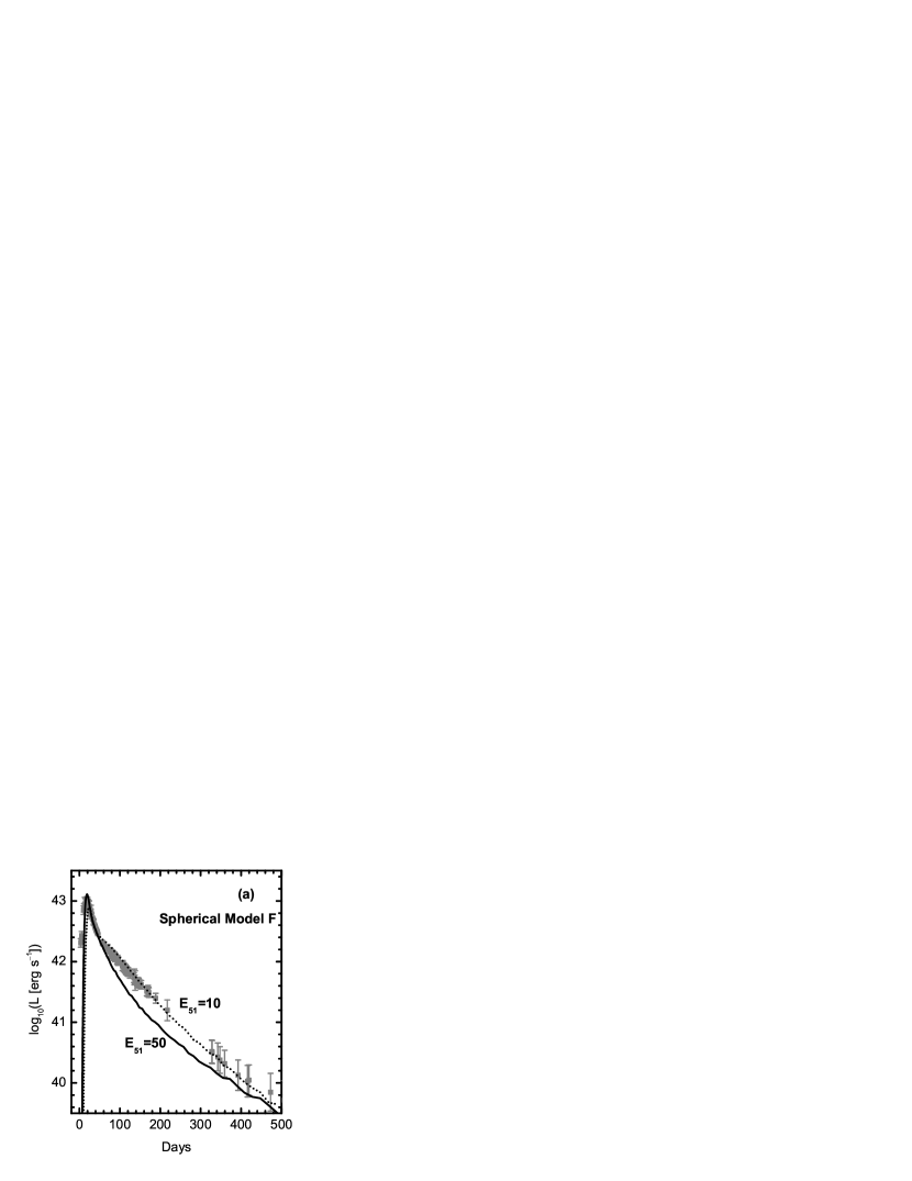
Figure 1: Light Curves for the spherical model F (Maeda et al. 2002) with the kinetic energy of the expansion $E_{51}\equiv E_{\rm K}/10^{51}=50$ (solid) and $10$ (dotted). The synthetic curves are obtained with $10^{6}$ photon packets. The bolometric UVOIR light curve of SN 1998bw is taken from Patat et al. (2001), with the distance modulus $\mu=32.76$ and the extinction $A_{V}=0.1$. The left panel (a) shows the light curve up to $500$ days, while the right panel (b) shows that up to only $50$ days.

The optical light curve could also be affected by the existence of asymmetry (Höflich et al. 1999; Maeda et al. 2003a). None of the spherical hydrodynamic models suggested to date can reproduce consistently the entire optical light curve of SN 1998bw, which is covered for a period of more than 1 year (see e.g., Nakamura et al. 2001). Figure 1 shows that the synthetic light curve for a spherical model with $E_{51}=50$ fits only the early phase, while one with $E_{51}=10$ fits only the late phase (see §4 for details). Only a priori parameterized spherical model fits both early and late phases (Chugai 2000; Maeda et al. 2003a), but no studies to date have investigated whether possible asphericity in SN 1998bw can improve the models, in particular with regard to the late phase optical light curve.

The aim of this paper is to provide theoretical predictions of observable signatures of asphericity in supernovae/hypernovae, and to verify whether the peculiarities of the prototypical hypernova SN 1998bw can be explained consistently from early to late phases. To add consistency to our study, we not only examine a light curve, but also spectroscopic signatures both in early and late phases. The contents of the present paper are the following. In §2, we describe a direct method to compute optical and gamma ray transport in asymmetric supernova ejecta. Explosion models for which we examine optical emission are also presented. In §3, radiation transport effects in aspherical supernovae are presented, and the differences from spherical models are discussed. In §4, synthetic light curves and their comparison to the observed light curve of SN 1998bw are presented. In §5, the expected photospheric velocities are compared with those of SN 1998bw. In §6, nebular spectra for the present models are presented. In §7, we close the paper with conclusions and discussion. Also in an Appendix, we describe the details of synthetic light curves, e.g., sensitivities on various assumptions.

2 METHOD AND MODELS

2.1 Gamma Ray and Optical Transport

We have developed a fully 3D, energy-dependent, and time-dependent gamma ray transport code. We will describe details of the gamma ray transport scheme in a subsequent paper (Maeda 2006b). In what follows, only a brief summary is presented.

The code has been developed following the individual packet method using a Monte Carlo scheme as suggested by Lucy (2005). The code follows gamma ray transport in SN ejecta discretised in 3D Cartesian grids and in time steps. For the ejecta dynamics, we assume homologous expansion, which should be a good approximation for SNe Ia/Ib/Ic. The expansion of the ejecta is taken into account by dealing with the Doppler shift, converting at every interaction a photon packet’s energy and direction between the comoving frame and the rest frame. The time delay between the emission of gamma rays and the final point (either absorption or escape out of the ejecta) is fully taken into account. Gamma ray lines from the decay chains ⁵⁶Ni $\to$ ⁵⁶Co $\to$ ⁵⁶Fe and ⁵⁷Ni $\to$ ⁵⁷Co $\to$ ⁵⁷Fe are included. For the interaction of gamma-rays with the SN ejecta, we consider pair production, Compton scattering (using the Klein-Nishina cross section), and photoelectric absorption (using cross sections from H to Ni).

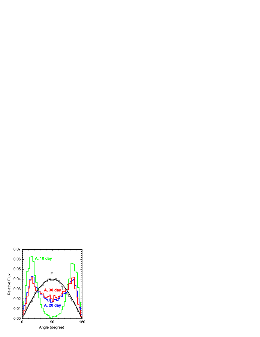
Figure 5: Angular distribution of the optical photons’ total energy content. The energy content of the optical photons (arbitrary scaled) is binned according to the polar angle $\theta$ of the last scattering point within the equal angle $4.5^{\rm o}$ each. Therefore, any spherically symmetric models should ideally give a sine curve (black). The distribution is shown for Model A at 10 (green), 20 (blue), and 30 days (red) after the explosion and for Model F (gray). The number of photons used in the computation is $10^{6}$.

In view of the recent investigation by Milne et al. (2004) showing that not all the published 1D gamma ray transport codes give mutually consistent results, we tested our new code by computing gamma ray spectra based on the (spherical) SN Ia model W7 (Nomoto, Thielemann, & Yokoi 1984), for which many previous studies are available for comparison. We compared our synthetic gamma ray spectra at 25 and 50 days with Figure 5 of Milne et al. (2004). We found excellent agreement between our results and the spectra resulting from most other codes, e.g. Hungerford, Fryer, & Warren (2003).

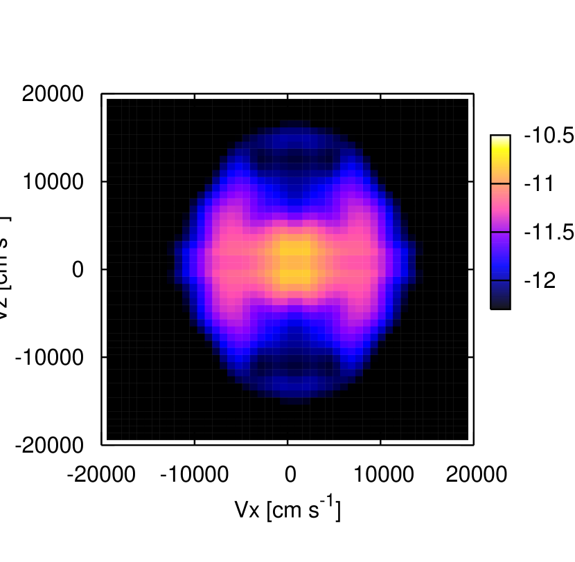
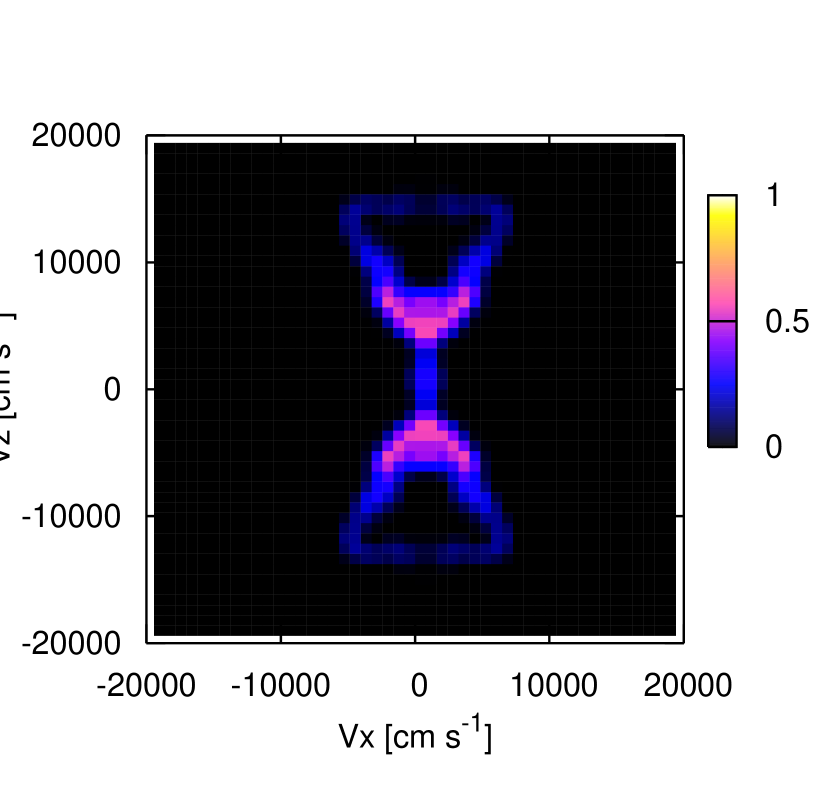
Figure 2: Model A (Maeda et al. 2002) with $E_{51}=10$. The left panel shows density distribution in a logarithmic scale ($\log(\rho~{}[{\rm g~{}cm}^{-3}])$) at 10 days after the explosion. The ejecta is already in a homologous expansion phase, so that the distribution is shown in the velocity space. The right panel shows mass fractions of ⁵⁶Ni in a linear scale.

Starting with the detailed gamma ray transport calculations, we compute optical bolometric light curves. We again follow the scheme presented in Lucy (2005) (see also Cappellaro et al. 1997). This is a fully time-dependent computation, taking into account the time delay between the creation of a photon from the deposition of a gamma ray and its escape from the ejecta. The transport is solved assuming a gray atmosphere, i.e., a frequency-independent opacity. We test the optical transport scheme by computing the light curve for the simplified SN model presented in Lucy (2005). For the test, we use a constant (both in space and time) opacity, same with the one used in Lucy (2005). We found good agreement between our light curve and Lucy (2005)’s Figure 2. For the optical opacity for aspherical supernova models presented in this paper, we phenomenologically use the formula given by Chugai (2000), i.e., $\kappa=0.13/[1+(t_{\rm d}/10)^{2}]$ cm² g^-1 where $t_{\rm d}$ is the time in day after the explosion. The formula was derived by computing opacity for the $13.8M_{\odot}$ CO star explosion model, including the contribution from electron scattering and bound-free transition, similar to the one used in Nakamura et al. (2001). By using the phenomenological formula, we miss detailed opacity distribution, and therefore a detailed light curve shape. Therefore, the detailed fit to the early phase light curve is beyond the scope of the present work (apparently, the late phase light curve is independent from the opacity prescription). This is mostly in order to save computational time (see also Lucy 2005).

Each packet is therefore followed by the Monte Carlo method consistently from its creation as a gamma ray to its escape from the ejecta as either a gamma ray or an optical photon. In this study, the ejecta are mapped onto a $60^{3}$ Cartesian grid. In total, $5\times 10^{6}$ photon packets (unless noted) with equal initial energy content are used to generate each synthetic optical light curve. When the packets escape from the ejecta, they are binned into 135 time steps, spaced logarithmically from 2 to 500 days, and into 10 angular zones with equal solid angle from $\theta=0^{\rm o}$ to $180^{\rm o}$ (here $\theta$ is the polar angle from the $z$-axis).

2.2 Models

We use Models A, C, and F of Maeda et al. (2002) to compute the optical emission. These are the explosions of a $16M_{\odot}$ He star (Nomoto & Hashimoto 1988) with explosion energy $E_{51}\equiv E_{\rm K}/10^{51}$ ergs $=10$. At the beginning of the calculations, the energy is deposited in the sphere for which $M_{r}=2.4M_{\odot}$. The asphericity of the explosion is obtained by depositing the energy more toward the polar direction ($z$-axis). Model F is a spherical model, and asphericity increases from Model C to Model A (see Maeda et al. 2002 for details).

To obtain (at least qualitatively) a good fit to SN 1998bw, we examined several models by rescaling the ejecta density and velocity self-similarly, so that $M_{\rm ej}\propto\rho v^{3}$ and $E_{\rm K}\propto M_{\rm ej}v^{2}$. According to previous results (Iwamoto et al. 1998; Nakamura et al. 2001), we always used models with $M_{\rm ej}=10.4M_{\odot}$, which is roughly expected for the explosion of a $\sim 13.8M_{\odot}$ CO star.

We did not independently change the mass of ⁵⁶Ni in the ejecta before computing light curve, since such a change would violate self-similarity in the synthetic light curve in terms of $E_{\rm K}$ and $M_{\rm ej}$. On the contrary, we obtained an approximate value of ⁵⁶Ni for each model by scaling the flux with the original $M$(⁵⁶Ni) to fit the observed luminosity. In the future we will examine light curves directly using values of $M_{\rm ej}$, $E_{\rm K}$, and $M$(⁵⁶Ni) obtained from hydrodynamic simulations of explosions with various parameters. Fine-tuning will be necessary to obtain a nice light curve, which is time-consuming. For example, the initial mass cut affects the final $M$(⁵⁶Ni). Accordingly, the initial mass cut should be fine-tuned to obtain the correct luminosity (see e.g., Maeda & Nomoto 2003b). Figure 2 shows the ejecta structure of Model A.

3 RADIATION TRANSPORT IN ASPHERICAL SUPERNOVAE

Figures 3 and 4 show the last scattering points of photon packets reaching an observer at any direction at a given epoch for Model A with $E_{51}=20$. Figure 5 shows the distribution of the total energy content of photon packets within position angle $\theta\sim\theta+d\theta$ as a function of the position angle of the points of last scattering. The figures were obtained from computational runs with $10^{6}$ photon packets (fewer than for the computations of the synthetic light curves). The fluctuation seen in Figure 5 is probably due to Monte Carlo noise.

The peak date of this model is $\sim 15-20$ days, with some variations depending on the viewing angle (§4). Figures 3 and 4 show that at 10 days only photons near the surface around the $z$-axis escape out of the ejecta. Virtually no photons are emitted from the equatorial region. In other words, these figures consist of two sector-shaped high temperature emitting regions, not even of a spheroid. At 20 days (near the time of peak), the last scattering points move deeper as well as diffuse to the equatorial region, so that they are distributed at all angles. The innermost oblate spheroid (or butterfly) shaped region (see also Fig. 2) is still very optically thick and allows no photons leakage. At 30 days the points move even deeper.

The peak date ($\sim 20$ days) almost coincides with the epoch when the distribution of last scattering points eventually covers the entire surface of the ejecta. This can be understood from the distribution of the heating source ⁵⁶Ni. Initially, the ejecta density is so high that gamma ray deposition closely follows the distribution of ⁵⁶Ni. The optical photons therefore start diffusing the ejecta from the two poles. As time goes by, the diffusion time scale becomes smaller and smaller. It becomes almost equal to the expansion time scale around the time of peak. Therefore, photons emitted near the $z$-axis can diffuse to the equator around the peak date. This is unlike the usual spherically symmetric view, where the peak date corresponds to the date when a photon emitted near the center can reach the surface. This characteristic behavior, i.e., the photosphere moving toward the equator, implies that the light curve (§4) and the spectroscopic characteristics (§5) before the peak will be differently affected by the viewing angle at different epochs.

Figure 5 also shows this behavior. At epochs approaching the peak (i.e., between 10 and 20 days) photons diffuse to the equator. After that (i.e., between 20 and 30 days), the distribution of the photons’ last scattering points does not evolve significantly. Note that the angular distribution of the photons is not spherically symmetric (as described by the sine curve overlapping with the spherically symmetric model F) even after the peak, but is concentrated toward the pole because of the high temperature resulting from a larger abundance of ⁵⁶Ni there.

4 OPTICAL LIGHT CURVES

We hereafter take the distance modulus $\mu=32.76$ (using the Hubble constant $H_{0}=72$ km s^-1 Mpc^-1 and the redshift 0.0085) and the extinction $A_{V}=0.1$ for SN 1998bw. Figure 1 shows optical bolometric light curves for the spherical model F. The model parameters are as follows: ($M_{\rm ej}$/$M_{\odot}$, $E_{51}$, $M$(⁵⁶Ni)/$M_{\odot}$) = (10.4, 10, 0.28), (10.4, 50, 0.40). The more energetic model ($E_{51}=50$) yields an early peak date, comparable to the observed one, while the less energetic model ($E_{51}=10$) peaks later than the observation. Although the rising part is not well fit even by the model with $E_{51}=50$ in the present study, extending the ⁵⁶Ni distribution out toward the surface would generate the rapid rise. (Note that in the present study we use the original ⁵⁶Ni distribution obtained from the hydrodynamic computation.) On the other hand, the late time light curve at $\sim 50-500$ days is more consistent with the less energetic model. After $\sim 50$ days the model with $E_{51}=50$ declines more rapidly than observed. A model with $E_{51}<10$, say $E_{51}\sim 7$ (Nakamura et al. 2001), would give a better fit to the late time light curve. This behavior of synthetic light curves is explained by simple scaling laws governing the peak date $t_{\rm peak}\propto(M_{\rm ej}^{3}E_{\rm K}^{-1})^{1/4}$ (Arnett 1982) and the late time gamma ray optical depth $\tau_{\gamma}\propto M_{\rm ej}^{2}E_{\rm K}^{-1}$ (Clocchiatti & Wheeler 1997; Maeda et al. 2003a). Note that similar light curves can be obtained by varying the mass and energy because of the above scaling properties. The degeneracy can be in principal solved by using another information such as velocities (§5 and 6).

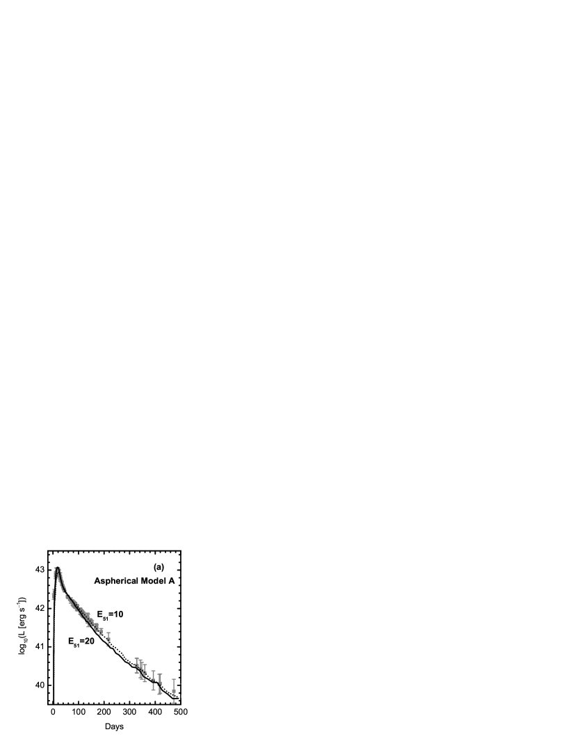
Figure 6: Light Curves for the aspherical model A (Maeda et al. 2002) with the kinetic energy of the expansion $E_{51}\equiv E_{\rm K}/10^{51}=20$ (solid) and $10$ (dotted). The observer’s direction is along the $z$-axis within $\theta<37^{\rm o}$. The synthetic curves are obtained with $5\times 10^{6}$ photon packets. The left panel (a) shows the light curve up to $500$ days, while the right panel (b) shows that up to only $50$ days.

Figure 6 shows optical bolometric light curves obtained for the aspherical model A. The model parameters are as follows: ($M_{\rm ej}$/$M_{\odot}$, $E_{51}$, $M$(⁵⁶Ni)/$M_{\odot}$) = (10.4, 10, 0.31), (10.4, 20, 0.39). The viewing angle is near the z-axis, within $37^{\rm o}$. Model C yields a light curve almost identical to Model A, with a slightly delayed peak date (1 or 2 days later than Model A for the same parameters).

The light curve shape of the aspherical models is different from that of the spherical model F (Fig. 1). For given $E_{51}$, the aspherical model peaks earlier than the spherical model F. This is due to the combined effects of (1) low densities along the $z$-axis resulting from the large isotropic energy and (2) extended ⁵⁶Ni distribution along the same direction. Photons therefore escape easily through the region near the $z$-axis (see also Figs. 3 – 5). Furthermore, the aspherical models yield more photons before the peak date than model F, while the latter shows a rather sudden rise around the peak with no modification of ⁵⁶Ni distribution. In a sense, the aspherical models naturally provide mixing of ⁵⁶Ni out to the surface (toward the $z$-axis) as a consequence of the hydrodynamic process (Maeda et al. 2002; Maeda & Nomoto 2003b), even without additional mixing processes such as Rayleigh-Taylor instabilities. At late phases, on the other hand, it resembles the spherical model with comparable or somewhat smaller total kinetic energy. For example, the aspherical model A with $E_{51}=10$ yields a late time light curve flatter than the corresponding model F with $E_{51}=10$. The decline rate is likely similar to the spherical model with $E_{51}\sim 7$ (Nakamura et al. 2001).

As a result, the light curve is very much improved for the aspherical models as compared with the spherical model F (Fig. 1). The aspherical models reproduce better the observations of SN 1998bw. Although we did not try to optimize the fit given the uncertainty and simplifications in our treatment of the optical opacities (§2), an aspherical model with $E_{51}\sim 10-20$ gives a nice fit.

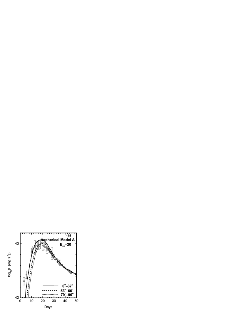
Figure 7: Dependence of the synthetic light curve on the viewing angle $\theta$ in Model A with $E_{51}=20$. The left panel (a) shows the synthetic light curves for different observer’s directions (solid for $0^{\rm o}<\theta<37^{\rm o}$, dashed for $53^{\rm o}<\theta<66^{\rm o}$, and dotted for $79^{\rm o}<\theta<90^{\rm o}$). The synthetic curves are obtained with $5\times 10^{6}$ photon packets. The right panel (b) shows the luminosities at different $\theta$ normalized by the mean luminosity $L_{\rm mean}$. Here $L_{\rm mean}$ is the luminosity averaged over all the solid angles (from $0^{\rm o}$ to $180^{\rm o}$).

Figure 7 shows how the viewing angle affects the light curve for Model A with $E_{51}=20$. The peak is earlier and brighter for an observer at a smaller viewing angle $\theta$ (angle from the $z$-axis). The ratio of the (apparent) luminosity for an observer on the $z$-axis to that for one on the equatorial plane, is close to 4 as the SN initially emerges around $\sim 5$ days after the explosion. The ratio then rapidly decreases to $\sim 1.2$ at the peak (around $\sim 20$ days). After the peak and up to $\sim 40$ days the ratio is almost constant and $\sim 1.2$, then it becomes unity as the whole ejecta become optically thin. For a less energetic model, the phase of constant ratio before the optically thin phase extends to later epochs (e.g., up to $\sim 50$ days for Model A with $E_{51}=10$).

To identify what causes this behavior we examined several models (see Appendix), and conclude as follows. Before the peak, the boost of the luminosity toward the $z$-direction is attributed to the fact that photons can only diffuse out to the $z$-direction (§3), i.e., that only the region around the $z$-axis is emitting photons. The cross sectional area of this photosphere is larger for an observer on the $z$-axis than on the $r$-plane, yielding a larger luminosity for the $z$-axis. As the peak date is approached, this region continues to expand toward the equator, making the luminosity difference for different directions smaller and smaller. After the peak, the angular distribution of the photosphere does not change very much any more, and the luminosity difference is almost constant. In this period, the central disk-like region absorbs $\gamma$-rays preferentially along the $z$-axis (because of the aspherical ⁵⁶Ni distribution), and emits optical photons preferentially toward the $z$-direction (because of the disk-like structure).

It is now interesting to compare our results to the previous work by Höflich et al (1999). Although the qualitative behavior, a brighter SN for smaller $\theta$, is mutually consistent, the details are different. First, our peak date depends on $\theta$ since the extended ⁵⁶Ni distribution along the $z$-axis allows different diffusion time scales for different $\theta$. This effect was simply not included in the previous work. Second, before the peak the behavior is different. Our model gives initially a very large enhancement of the luminosity toward the $z$-axis, then the effect gradually decreases toward the peak date. On the other hand, Höflich et al. (1999) gave an almost constant factor of the boost until the peak is reached, and after that the factor decreases by about a factor of 2 in 2 weeks (their Figure 6).

The reason can be seen in the difference of the mechanism of boosting luminosity. Although in our models this is done by diffusing photons from $z$-direction to the equatorial direction, in Höflich et al. (1999) boosting luminosity is always attributed to an oblate spheroidal photosphere. Note that the input models are different. Their parameterized models deviate greatly from spherically symmetry, so that the axis ratio of the photosphere is always (from the innermost region to the outermost region) $\sim 2$ (see Fig. 4 of Höflich et al. 1999). In outer regions such as $v\mathrel{\hbox to0.0pt{\lower 4.0pt\hbox{\hskip 1.0pt$\sim$}\hss}\raise 1.0pt\hbox{$>$}}10,000$ km s^-1 (depending on $E_{51}$) the density does not largely deviate from spherical symmetry in our models. Only below this the density contour shows a disk like structure (Fig. 2), but with a smaller axial ratio than theirs. Finally, in our model the difference in luminosities for different $\theta$ is much smaller than theirs after the peak. In this phase, the boost of the luminosity is attributed to both the aspherical ⁵⁶Ni distribution and the disk-like density structure (see above), while in Höflich et al. (1999) it is due only to the disk-like structure. The degree of the boost is smaller for our model than Höflich et al. (1999) partly because the deviation of the ejecta density distribution from spherical symmetry is smaller in our models, although the direct comparison is difficult because the mechanism is different. Also, the low angular resolution for small $\theta$ in the present calculations (i.e., averaging the interval $0^{\rm o}\sim 37^{\rm o}$) may also smooth the luminosity difference to some extent. This is due to the current choice of an equal solid angle for photon binning, which is most efficient in the Monte-Carlo scheme. In the future, we will use finer bins with a larger number of photon packets. In any case, this resolution effect is probably small.

Of course, which models are more realistic is a different question. Although our models are based on hydrodynamic computations (in this sense our models are at least more self-consistent), different parameters for explosion calculations may lead to density structure more similar to Höflich et al. (1999). Actually, most of the differences may be understood in terms of the different progenitors (the ejecta mass $\sim 2$ and $10M_{\odot}$, for Höflich et al. (1999) and the present study, respectively). One may expect larger asphericity in the inner region for low mass cores.

In any case, we emphasize that it is very important to treat the ⁵⁶Ni distribution correctly and the gamma ray transport in 3D, as this is in the present model the main cause of the characteristic behavior of the light curves. Also, we would suspect based on our result and analysis that the naive guess that larger asphericity (by a jet powered explosion) always yields a larger luminosity boost toward the $z$-axis may not be correct. For example, if ⁵⁶Ni-rich blobs penetrate entirely through the star as an extreme case of a jet powered explosion, then the SN could be brighter near the $r$-plane than on the $z$-axis because two blobs are seen from the $r$-plane but just one from the $z$-axis. In our model the blobs are stopped in the star and therefore the SN is brighter on the $z$-axis. In any case, light curve behavior is highly sensitive to density and ⁵⁶Ni distribution, and therefore one should always be careful when deriving asphericity (if possible) from the light curve. One should always check the consistency with other information, e.g., spectroscopic characteristics, as we proceed to do in subsequent sections.

5 PHOTOSPHERIC VELOCITIES

A model can be further constrained from its spectroscopic characteristics. For example, the evolution of the photospheric velocity provides important information since it scales roughly as $v_{\rm ph}\propto\sqrt{E_{\rm K}/M_{\rm ej}}$, while the light curve shape depends on these parameters differently (§4).

The concept of the photosphere needs careful reconsideration if the ejecta are not spherically symmetric. Deriving the photospheric velocity from observed spectra, in fact, implicitly assumes that the ejecta are spherically symmetric. An absorption minimum corresponds to the line-of-sight velocity of a slice (perpendicular to an observer) where the amount of absorption takes a maximum value. In the spherically symmetric case, this velocity is exactly what is called the photospheric velocity, but in an asymmetric geometry this may not be the case. Therefore, direct comparison between a multi dimensional model and observations ultimately needs multi dimensional (early phase) spectrum synthesis computations (e.g., Kasen et al. 2004), which are beyond the scope of the present paper.

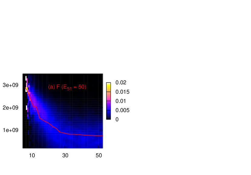
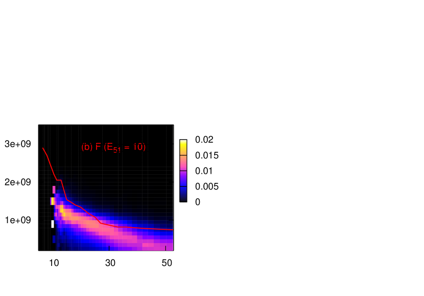
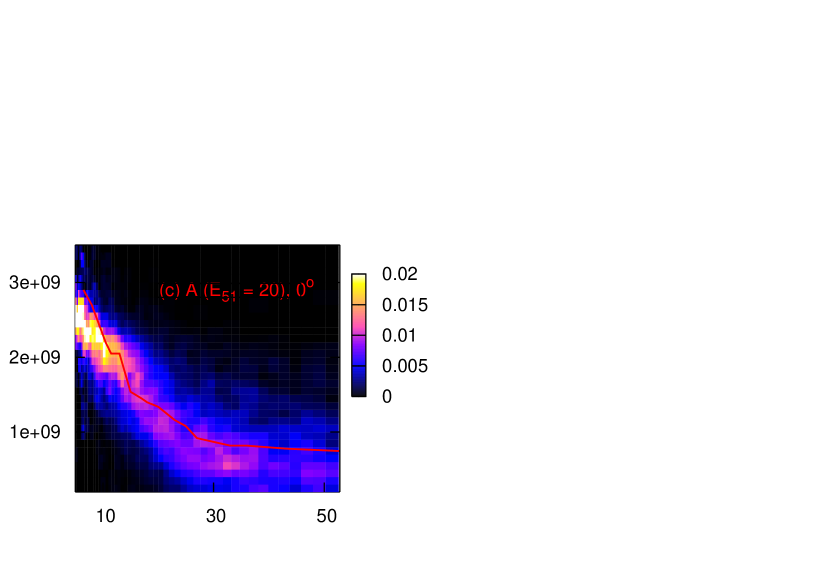
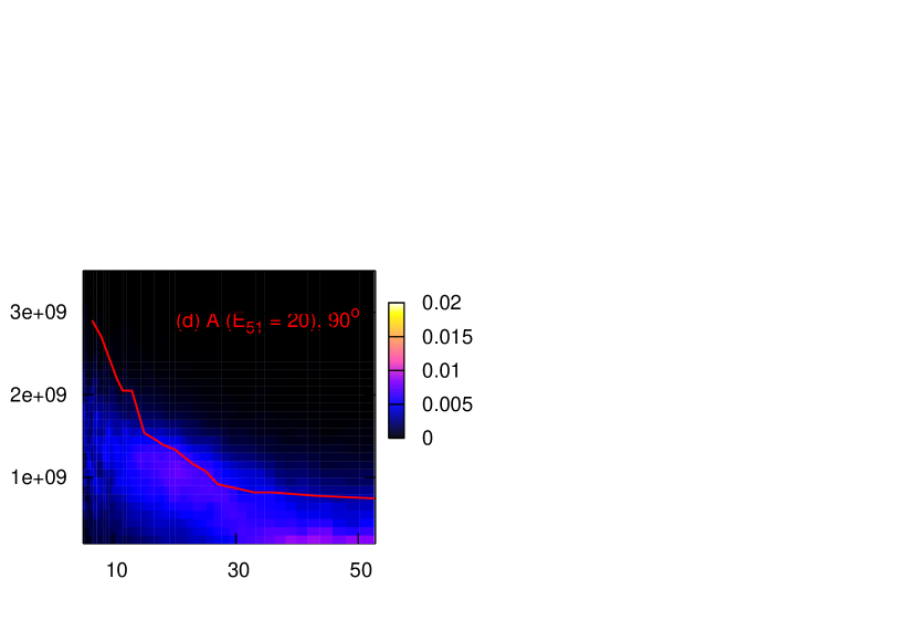
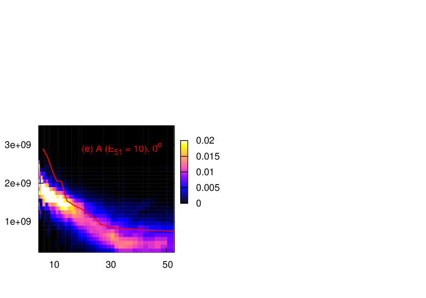
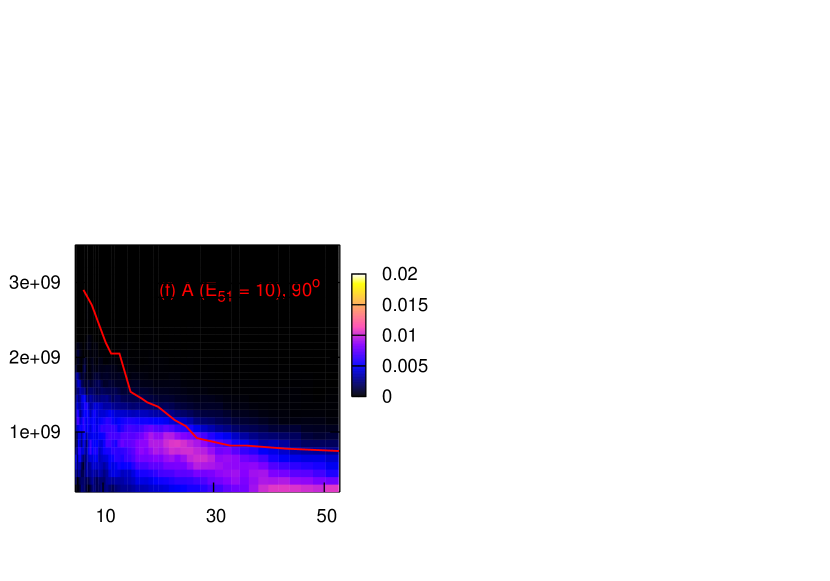
Figure 8: Time evolution (horizontal axes) of distribution of photon’s energy contents as a function of line-of-sight velocities (vertical axes) at the last scattering points. The bright regions give a rough estimate of photospheric velocities as a function of time. See §5 for details. The distribution is shown for (a) the spherical model F with $E_{51}=50$, (b) F with $E_{51}=10$, (c) the aspherical model A with $E_{51}=20$ and $\theta=0^{\rm o}$, (d) A with $E_{51}=20$ and $\theta=90^{\rm o}$, (e) A with $E_{51}=10$ and $\theta=0^{\rm o}$, and (c) A with $E_{51}=10$ and $\theta=90^{\rm o}$. Here $\theta$ is the polar angle (from the $z$-axis) of the observer’s direction. Also shown is the photospheric velocity of SN 1998bw as a function of time (curve; Patat 2001).

We give a very rough estimate of the photospheric velocity by looking at the line-of-sight velocity of the last scattering points of optical photons emitted toward a given observer’s direction. Figure 8 shows the photons’ energy content distribution as functions of the line-of-sight velocity of the last scattering points and of the epoch. The brightest part gives a rough estimate of the photospheric velocity. By definition the photospheric velocity in spherically symmetric ejecta is the line-of-sight velocity of the (nearly) last scattering point moving toward the observer, while Figure 8 shows the line-of-sight velocity of ”all” the last scattering points from which photons are emitted in the direction to the observer. Therefore, taking into account photons emitted aside the line connecting the observer and the center of the SN ejecta, this distribution will probably somewhat underestimate the photospheric velocity. Also, the velocity is apparently sensitively affected by the optical opacity, therefore uncertainty in the opacity leads to uncertainty in the photospheric velocity.

Given the above caveat, Figure 8 shows that the spherical model F with $E_{51}=50$ gives a photospheric velocity consistent with SN 1998bw. Model F with the smaller energy ($E_{51}=10$) gives a velocity smaller than observed. The aspherical model A yields different ”photospheric” velocities for different directions as well as different luminosities for different directions. Especially before the peak there is a large velocity boost toward the $z$-axis compared to the corresponding spherical model with the same energy. Indeed, Model A with $E_{51}=20$ gives a velocity for the $z$-axis before the peak similar to that of Model F with $E_{51}=50$.

Figure 8 shows that Model A with $E_{51}=20$ is consistent with SN 1998bw. The model A with $E_{51}=10$ gives a bit smaller velocity before $\sim 15$ days. However, it should be stated that in Model A with $E_{51}=10$, the maximum velocity in the ejecta is $\sim 20,000$ km s^-1. Because the decreasing density near the surface is difficult to follow correctly in 2D/3D hydrodynamic simulations, we might be underestimating the density at $\mathrel{\hbox to0.0pt{\lower 4.0pt\hbox{\hskip 1.0pt$\sim$}\hss}\raise 1.0pt\hbox{$>$}}20,000$ km s^-1. After the peak the photosphere moves deeper and this uncertainty is not a problem. If we judge the model photospheric velocity at the peak, even Model A with $E_{51}=10$ may marginally be consistent with the observation. Therefore, the aspherical model A with $E_{51}=10\sim 20$ is consistent with the observed photospheric velocities, assuming the observer is placed near the $z$-direction.

6 NEBULAR SPECTRA

After the ejecta become optically thin, the SN evolves into the nebular phase. The emission process is now different from the earlier photospheric phase. For the nebular phase a 3D spectrum synthesis method has already been developed (Kozma et al. 2005; Maeda et al. 2006a). We compute the nebular emission at 350 days after the explosion for the present models. The detail of the nebular emission computation in 3D and its application to SN 1998bw are presented in Maeda et al. (2006a). In Maeda et al. (2006a), the mass of some elements are modified independently to obtain a detailed fit, while in this work we do not allow this. Because in this paper we rescale the hydrodynamic models somewhat differently, we again compute nebular spectra for the present models to test consistency.

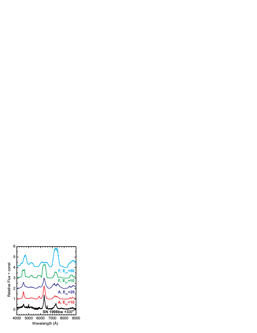
Figure 9: Synthetic nebular spectra (at 350 days after the explosion) for Model F with $E_{51}=50$ (cyan), F with $E_{51}=10$ (green), Model A with $E_{51}=20$ (blue), and A with $E_{51}=10$ (red). The viewing angle is $30^{\rm o}$ from the $z$-axis for Model A. Also shown is the observed spectrum of SN 1998bw at 337 days after the maximum brightness (black).

Figure 9 shows synthetic nebular spectra for the present models at $350$ days after the explosion as compared with the observed spectrum of SN 1998bw at $337$ days after the peak (Patat et al. 2001). Although no attempt has been made to obtain a good fit to SN 1998bw, the aspherical model A is at least qualitatively consistent with the observation. For example, no spherical models give the sharply peaked [OI] 6300, 6363Å doublet, the strongest line, as is observed (e.g., Sollerman et al. 2000; Mazzali et al. 2001). On the other hand, the aspherical model A with $E_{51}=10\sim 20$ yields the sharply peaked [OI] line, with a viewing angle close to the $z$-axis as is consistent with the light curve (§4), with photospheric velocity analysis (§5), and with the detection of a GRB. See Maeda et al. (2002, 2006a) for details. The observed nebular line broadness agrees well with Model A with $E_{51}=10$, but is a bit narrower than the synthetic lines of Model A with $E_{51}=20$. This may possibly imply a less massive progenitor for SN 1998bw than examined in the present study ($M_{\rm ms}=40M_{\odot}$), which is further discussed in §7.

7 CONCLUSIONS AND DISCUSSION

The aims of this paper are (1) to examine the optical properties of aspherical supernovae, including light curves covering more than $1$ year, early phase photospheric velocities, and late phase nebular spectra, and (2) to investigate if one can obtain a model consistent with hypernova SN 1998bw in all these aspects. We have presented observational signatures expected from aspherical hypernova models of Maeda et al. (2002) and closely compare them with observations of SN 1998bw.

We use a Monte Carlo scheme to solve the time-dependent radiation transport problem in homologously expanding SN ejecta in 3D grids. It is demonstrated that the scheme is very suitable to the problem. For example, the concept of the last scattering points, which can easily be traced in the Monte Carlo scheme, turns out to be very useful to understand the physical reasons of some non-trivial behaviors in time-dependent 3D radiation transport (see e.g., Appendix).

The light curves of the aspherical models show characteristics different from those of spherical models. The aspherical model A (or C) of Maeda et al. (2002) shows both (1) early emergence of optical emission and (2) boosted luminosity toward the $z$-axis before the peak. These are mainly attributed to concentration of ⁵⁶Ni along the $z$-axis. The degree of boosting on the $z$-axis relative to the $r$-axis decreases with time, from a factor of $\sim 4$ to $\sim 1.2$. After the peak and until the nebular phase, the boosting is smaller than at earlier phases. In this phase, the ratio of the luminosity in the $z$-axis to that on the $r$-plane remains almost constant at $\sim 1.2$. The photospheric velocity is dependent on the viewing angle, and is higher on the $z$-axis than on the $r$-plane. Model A with $E_{51}=20$ gives photospheric velocities comparable to those of the spherical model F with $E_{51}=50$. Nebular spectra are also different for different asphericity and different viewing angle. If the aspherical model is viewed on the $z$-axis, it yields sharply peaked O and Mg lines, and broad Fe lines (see Maeda et al. 2006a for more detail).

All these features are consistent with the observations of SN 1998bw. Note that these properties could not be explained in spherically symmetric models. The highly aspherical model (A or C in Maeda et al. (2002)) with $M_{\rm ej}\sim 10M_{\odot}$, $M$(⁵⁶Ni) $\sim 0.4M_{\odot}$, and $E_{51}=10\sim 20$ gives a nice fit to all these observations. Strictly speaking, there is still a small difficulty, i.e., the early phase observations favor the larger energy $E_{51}=20$ (§4 and 5) although the late phase observations favor the smaller energy $E_{51}=10$ (§4 and 6). However, given the fact that we use the ”hydrodynamic” model, the situation is much better than in the spherical models (i.e., $E_{51}=7$ vs. $E_{51}=50$; see Nakamura et al. 2001). For example, if Model A with $E_{51}=10$ has more high velocity materials with some ⁵⁶Ni at $V>20,000$ km s^-1 than found in the hydrodynamic simulation (see discussion in §5), then the problems in the early phase (a somewhat late peak and smaller photospheric velocity than observed) may be resolved. This will lead to an increased expansion kinetic energy, and $E_{51}\sim 20\pm 5$ may be a solution. Another possibility is that the progenitor may be less massive than examined in the present study. A less massive star tends to be compact in inner regions and to be extended in outer regions, so that it may yield average velocities higher in the early phases (i.e., outer parts) and lower in the late phases (i.e., inner parts) than a more massive star. However, it is unlikely that the progenitor’s mass is very different from $M_{\rm ms}=40M_{\odot}$ since then the photospheric velocity will not follow the observations. In any case, it is an interesting possibility and should be addresses in future studies. Apparently, to do this it is necessary to compute hydrodynamics of the explosions for various progenitors rather than scaling the mass and energy, since the different density distribution will be an important factor.

The mass of ⁵⁶Ni $\sim 0.4M_{\odot}$ is consistent with the result of the aspherical explosion model of Maeda et al. (2002), where initial mass cut is set at $M_{r}=2.4M_{\odot}$ and all the ⁵⁶Ni is produced by explosive nucleosynthesis in the shock waves propagating the progenitor star. If the initial mass cut (initial remnant mass) is larger, another mechanism such as a massive disk wind (MacFadyen 2003) is necessary. In either case, the nucleosynthesis products are suggested to be different from conventional spherically symmetric models (e.g., Nagataki 2000; Maeda et al 2002; Maeda & Nomoto 2003b; Prute, Surman, & McLaughlin 2004a; Pruet, Thompson, & Hoffman 2004b). Some elements such as Zn, Ti are suggested to be enhanced. This could have a very important consequence on the Galactic chemical evolution (e.g., Kobayashi et al. 2006), especially at earliest phases (e.g., Iwamoto et al. 2005). These nucleosynthetic features could be examined by observing abundance patterns of either extremely metal poor halo stars (e.g., Christlieb et al. 2002; Frebel et al. 2005) or binary systems having experienced a supernova explosion of the primary star (e.g., Podsiadlowski et al. 2002; González Hernández et al. 2005).

A viewing angle $\theta<30^{\rm o}$ is found to be consistent with, indeed even favorable for, the observed optical light curve of SN 1998bw. This is consistent with the result of Höflich et al. (1999). The result seems very natural given the detection of a gamma ray burst in association with SN 1998bw. This is also consistent with a somewhat ”off-axis” jet model ($\theta\sim 15^{\rm o}$; Yamazaki, Yonetoku, & Nakamura 2003) suggested for SN 1998bw. Placing tighter constraints on the viewing angle from models of the optical emission is unfortunately difficult, since the optical emission comes from non-relativistic ejecta which do not show relativistic boosting.

Comparison of our models with other supernovae, including hypernovae SN 1997ef and 2002ap, should be interesting. Late time light curves of SNe 1997ef (e.g., Mazzali, Iwamoto, & Nomoto 2000) and 2002ap (e.g., Mazzali et al. 2002) are also inconsistent with spherical models (see e.g., Maeda et al. 2003a). To solve the problem in these SNe will need extensive survey of $M_{\rm ej}$, $E_{51}$, $M$(⁵⁶Ni), and the ejecta geometry (the degree of asphericity). Qualitatively, they deviate from the prediction of spherically symmetric model in the same manner as SN 1998bw did, so that asphericity is a promising candidate to solve the discrepancy. If it is, then asphericity is a general property of hypernovae. Indeed, the asphericity is likely a general feature of core-collapse supernovae. There are some supernovae, probably of normal energy, that possibly show a similar light curve behavior (e.g., Clocchiatti et al. 1996; Clocchiatti & Wheeler 1997). A direct Hubble Space Telescope image of SN 1987A clearly shows bipolarity (Wang et al. 2002). Also, polarization and spectropolarization measurements suggest that core-collapse supernovae are essentially asymmetric (Wang et al. 2001; Leonard, Filippenko, & Ardila 2001). If available, modeling not only light curves, but also nebular spectra (e.g., Matheson et al. 2001) is very important to constraint the nature of the explosion (see also Mazzali et al. 2005) as we see in the present paper.

Also interesting is the high energy emission from aspherical supernovae/hypernovae. It should be noted that computations of high energy emission based on the present model give model predictions ”consistent” with optical observations of hypernova SN 1998bw. This consistent modeling between optical and high energy emissions has only been done for the very nearby SN 1987A (e.g., McCray, Shull, & Sutherland 1987; Woosley et al. 1987; Shibazaki, & Ebisuzaki 1988; Kumagai et al. 1989). Because a hypernova is potentially a very interesting event not only in optical but also in $X$ and $\gamma$ rays because of a large amount of radioactivity (especially ⁵⁶Ni: see e.g., Nomoto et al. 2004) and large kinetic energy, model predictions consistent with the optical observations should be provided. We will present $X$ and $\gamma$ ray emission for the present models in a subsequent paper (Maeda 2006b).

Appendix A DETAILS OF SYNTHETIC LIGHT CURVES

In this section, we examine several models based on Model A with $E_{51}=20$. We examine how the following factors affect the synthetic light curves. (1) Distribution of ⁵⁶Ni. (2) Treatment of time duration of a photon packet spent in the ejecta.

Taking Model A with $E_{51}=20$, (1) we assume that all the ⁵⁶Ni is at the center, while the density structure is unchanged (we call this case ”central ⁵⁶Ni”). This is an approximation to the case where the ⁵⁶Ni is always deeper than the photosphere. (2) We assume that the diffusion time has no angular dependence. We further assume $L_{\theta}(t)=f(\theta,t)L_{\rm mean}(t)$, where the mean luminosity $L_{\rm mean}(t)$ is assumed to be that of the corresponding ”spherical” model with the same $M_{\rm ej}$, $M$(⁵⁶Ni), and $E_{51}$, and $f(\theta,t)$ is the angular distribution of emitted photons at fixed time $t$ (assuming that the photon diffusion time at any angle is equal to that of the spherical model). These assumptions in the case (2) are used in the previous work by Höflich et al. (1999) (we call this case ”Approximate diffusion”).

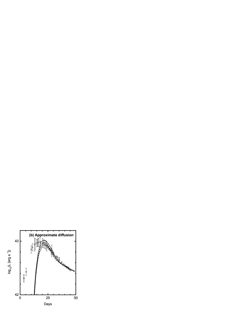
Figure 11: Synthetic light curves for the model A with $E_{51}=20$ with various assumptions, i.e., (a) ”⁵⁶Ni centered”, (b) ”Approximate diffusion”, and (c) ”⁵⁶Ni centered and Approximate diffusion”. See the caption of Figure 10 for details. The masses of ⁵⁶Ni in the models are $0.27M_{\odot}$ (Case a) and $0.29M_{\odot}$ (Cases b and c) (Note, however, that in Appendix we do not attempt to derive the mass of ⁵⁶Ni).

Following three cases are examined. (a) The central ⁵⁶Ni distribution, using the ”correct” angle dependent diffusion time fully computed with a time-dependent 3D computation (”central ⁵⁶Ni”), (b) the original ⁵⁶Ni distribution, using the non-angle dependent diffusion time as described above (”Approximate diffusion”), and (c) the central ⁵⁶Ni and non-angle dependent diffusion, which is probably most similar to the case examined in Höflich et al. (1999) (”⁵⁶Ni centered + Approximate diffusion”). Figures 10 and 11 show the angular luminosity distribution and light curves, respectively. Figures 12 – 14 show the cross sectional view (on the $V_{x}-V_{z}$ plane) of the last scattering points for optical photon packets.

How the ⁵⁶Ni distribution affects the light curve appearance is seen by comparing Figures 7a and 7b (with original aspherical distribution) with Figures 10a and 11a (with ⁵⁶Ni centered distribution). The effects of treatment of diffusion time is seen by comparing Figures 7a and 7b [10a and 11a] (directly solving 3D transport) with Figures 10b and 11b [10c and 11c] (with the approximate diffusion).

First, we found that the aspherical distribution of ⁵⁶Ni, extending toward the surface along the $z$-axis, is important to make the early emergence of optical photons before the peak. All three models show the evolution of the light curves around the peak much slower than the original model (§4). Note that even Case b using the original ⁵⁶Ni distribution for computing the angle dependence is in effect similar to the ⁵⁶Ni centered models (a and c), because of the assumption $L_{\rm mean}=L_{\rm spherical}$ where the spherical model shows more or less centered ⁵⁶Ni distribution. Also interesting is that the models with the original ⁵⁶Ni distribution (original and Case b) show the boost of luminosity toward the $z$-axis before the peak, while the ones with the centered ⁵⁶Ni distribution (Cases a and c) do not. Note that while Case a apparently shows a luminosity boost before the peak in Figure 10a, this effect disappears well before the peak so that the effect is not seen in Figure 11a. A close view of the last scattering points (Figures 4 and 12 – 14) suggests that before the peak the boost of the luminosity toward the $z$-axis can mainly be attributed to the aspherical ⁵⁶Ni distribution and energy deposition (with minor contribution due to low densities and small diffusion time scale along the $z$-axis).

Second, we found that the treatment of the diffusion time scale is also very important. Especially we point out that the assumption that $L_{\rm mean}(t)$ is equal to the corresponding ”spherical” model is not always correct. It ignores the fact that the ⁵⁶Ni distribution is different for the aspherical and spherical models. For example, comparing the original model with Case b demonstrates that the ”mean” luminosity computed for the original model is not similar to the corresponding spherical model.

Finally, all the three cases as well as the original model (§4) show an almost constant factor of boosting luminosity after the peak, and this effect is especially evident for Case a and c (⁵⁶Ni centered). A close view of the last scattering points illustrates that for Cases a and c at these epochs the photosphere is an oblate or disk-like spheroid with larger cross sectional area for smaller viewing angle $\theta$ as suggested by Hölich et al (1999). However, the original model and Case b with the original aspherical ⁵⁶Ni distribution show the distribution of the last scattering points preferentially along the $z$-axis. If the ⁵⁶Ni is distributed along the $z$-axis, $\gamma$-rays are absorbed preferentially along the $z$-axis, making temperature higher toward the $z$-axis. Because this high temperature spots are on the disk-like structure, they emit more toward the $z$-axis than the $r$-axis.

From these test calculations, we conclude that the behavior of the synthetic light curve of our aspherical models can be understood as follows. First, the angular dependence can be divided into two phases, i.e., before and after the peak. Before the peak, boosting luminosity toward the $z$-axis is mainly attributed to the aspherical ⁵⁶Ni distribution. After the peak, it is caused by combined effects of the aspherical ⁵⁶Ni distribution and the disk-like inner structure. The fact that all the three models give light curves different from the original model A, especially in reproducing the rapid rise before the peak, demonstrates the importance of direct time dependent computations of light curves without crude approximation on the transport processes.

Figure 3: Last scattering points of optical photon packets escaping out of the ejecta in Model A with $E_{51}=20$ at $10$ (left) and $20$ (right) days after the explosion. The points are shown in the velocity space ($V_{x}$,$V_{y}$,$V_{z}$ [cm s^-1]) and the vertical axis is the $V_{z}$ axis. The total number of optical photons packets is $10^{6}$.

Figure 4: Last scattering points of optical photon packets escaping out of the ejecta in Model A with $E_{51}=20$ shown in the $V_{x}-V_{z}$ plane (i.e., the slice at $V_{y}=0$). The vertical and horizontal axes are respectively the $V_{z}$ and the $V_{x}$ axes. The last scattering points with $-2<V_{y}/10^{8}{\rm cm\ s}^{-1}<2$ are shown. The distribution is shown for $10$, $20$, $30$, and $40$ days after the explosion.

Figure 10: Synthetic light curves normalized by the mean luminosity $L_{\rm mean}$, depending on the viewing angle $\theta$ (solid for $0^{\rm o}<\theta<37^{\rm o}$, dashed for $53^{\rm o}<\theta<66^{\rm o}$, and dotted for $79^{\rm o}<\theta<90^{\rm o}$) for Model A with $E_{51}=20$. Here $L_{\rm mean}$ is the luminosity averaged over all the solid angles (from $0^{\rm o}$ to $180^{\rm o}$). Three cases are shown: The panel (a) shows the model with ⁵⁶Ni distribution (artificially) concentrated at the center (”⁵⁶Ni centered”). The panel (b) shows the model with the assumptions $L_{\rm mean}=L_{\rm spherical}$ (a spherical model with the same energy) and no-angle dependent diffusion time (”Approximate diffusion”; See Appendix for details). The panel (c) shows the model with all the assumptions in (a) and (b). The models are computed with $10^{6}$ photon packets.

Figure 12: Last scattering points for Model A with $E_{51}=20$, with ⁵⁶Ni distribution (artificially) concentrated at the center (”⁵⁶Ni centered”). Last scattering points of optical photon packets are shown in the $V_{x}-V_{z}$ plane (i.e., the slice at $V_{y}=0$). The vertical and horizontal axes are respectively the $V_{z}$ and the $V_{x}$ axes. The last scattering points with $-2<V_{y}/10^{8}{\rm cm\ s}^{-1}<2$ are shown. The distribution is shown for $15$, $20$, $30$, and $40$ days after the explosion.

Figure 13: Last scattering points for Model A with $E_{51}=20$, with the assumptions $L_{\rm mean}=L_{\rm spherical}$ and no-angle dependent diffusion time (”Approximate diffusion”; See Appendix for details). Last scattering points of optical photon packets are shown in the $V_{x}-V_{z}$ plane (i.e., the slice at $V_{y}=0$). The vertical and horizontal axes are respectively the $V_{z}$ and the $V_{x}$ axes. The last scattering points with $-2<V_{y}/10^{8}{\rm cm\ s}^{-1}<2$ are shown. The distribution is shown for $10$, $20$, $30$, and $40$ days after the explosion.

Figure 14: Last scattering points for Model A with $E_{51}=20$ with ⁵⁶Ni distribution (artificially) concentrated at the center, with the assumptions $L_{\rm mean}=L_{\rm spherical}$ and no-angle dependent diffusion time (”⁵⁶Ni centered” and ”Approximate diffusion”; See Appendix for details). Last scattering points of optical photon packets are shown in the $V_{x}-V_{z}$ plane (i.e., the slice at $V_{y}=0$). The vertical and horizontal axes are respectively the $V_{z}$ and the $V_{x}$ axes. The last scattering points with $-2<V_{y}/10^{8}{\rm cm\ s}^{-1}<2$ are shown. The distribution is shown for $10$, $20$, $30$, and $40$ days after the explosion.

References

- (1) Arnett, W.D. 1982, ApJ, 253, 785
- (2) Brown, G.E., Lee, C.-H., Wijers, R.A.M.J., Lee, H.K., Israelian, G., & Bethe, H.A. 2000, New Astronomy, 5, 191
- (3) Cappellaro, E., Mazzali, P.A., Benetti, S., Danziger, I.J., Turatto, M., Della Valle, M., & Patat, F. 1997, A&A, 328, 203
- (4) Christlieb, N., et al. 2002, Nature, 419, 904
- (5) Clocchiatti, A., Wheeler, J.C., Benetti, S., & Frueh, M. 1996, ApJ, 459, 547
- (6) Clocchiatti, A., & Wheeler, J.C. 1997, ApJ, 491, 375
- (7) Chugai, N.N. 2000, Astronomy Letters, 26, 797
- (8) Deng, J., Tominaga, N., Mazzali, P.A., Maeda, K., & Nomoto, K. 2005, ApJ, 624, 898
- (9) Filippenko, A.V., et al. 1995, ApJ, 450, L11
- (10) Frebel, A., et al. 2005, Nature, 434, 871
- (11) Fryer, C.L., & Warren, M.S. 2004, ApJ, 601, 391
- (12) Galama, T.J., et al. 1998, Nature, 395, 670
- (13) Gamezo, V. N., Khokhlov, A.M., & Oran, E.S. 2005, ApJ, 623, 337
- (14) González Hernández, J.I., Rebolo, R., Israelian, G., Casares, J., Maeda, K., Bonifacio, P., & Molara, P. 2005, ApJ, 630, 495
- (15) Hjorth, J., et al. 2003, Nature, 423, 847
- (16) Höflich, P. 1991, A&A, 246, 481
- (17) Höflich, P. 1995, ApJ, 440, 821
- (18) Höflich, P., Wheeler, J.C., & Wang, L. 1999, ApJ, 521, 179
- (19) Hungerford, A.L., Fryer, C.L., & Warren, M.S. 2003, ApJ, 594, 390
- (20) Iwamoto, K., et al. 1998, Nature, 395, 672
- (21) Iwamoto, N., Umeda, H., Tominaga, N., Nomoto, K., & Maeda, K. 2005, Science, 309, 451
- (22) Janka, H.-Th., Scheck, L., Kifonidis, K., Müller, E., & Plewa, T. 2005, in ”The Fate of the Most Massive Stars”, ASP Conference Proceedings, (eds. P. Humphreys and K. Stanek), vol. 332, 372
- (23) Kasen, D., Nugent, P., Thomas, R.C., & Wang, L. 2004, ApJ, 610, 876
- (24) Kawabata, K.S., et al. 2003, ApJ, 593, L19
- (25) Kobayashi, C., et al. 2006, ApJ, submitted
- (26) Kozma, C., et al. 2005, A&A, 437, 983
- (27) Kumagai, S.,Shigeyama, T., Nomoto, K., Itoh, M., Nishimura, J., & Tsuruta, S. 1989, ApJ, 345, 412
- (28) Leonard, D.C., Filippenko, A.V., & Ardila, D.R. 2001, ApJ, 553, 861
- (29) Lucy, L.B. 2005, A&A, 429, 19
- (30) MacFadyen, A. I., & Woosley, S. E. 1999, ApJ, 524, 262
- (31) MacFadyen, A.I. 2003, in ’From Twilight to Highlight: The Physics of Supernovae’, eds. W. Hillebrandt & B. Leibundgut (Berlin: Springer), 97
- (32) Maeda, K., Nakamura, T., Nomoto, K., Mazzali, P.A., Patat, F., & Hachisu, I. 2002, ApJ, 565, 405
- (33) Maeda, K., Mazzali, P.A., Deng, J., Nomoto, K., Yoshii, Y., Tomita, H., & Kobayashi, Y. 2003a, ApJ, 593, 931
- (34) Maeda, K., & Nomoto, K., 2003b, ApJ, 598, 1163
- (35) Maeda, K., Nomoto, K., Mazzali, P.A., & Deng, J. 2006a, ApJ, 640, in press (astro-ph/0508373)
- (36) Maeda, K. 2006b, ApJ, 644, in press (astro-ph/0511480)
- (37) Matheson, T., Filippenko, A.V., Leonard, D.C., & Shields, J.C. 2001, AJ, 121, 1648
- (38) Matheson, T., et al. 2003, ApJ, 599, 394
- (39) Mazzali, P.A., Iwamoto, K., & Nomoto, K. 2000, ApJ, 545, 407
- (40) Mazzali, P.A., Nomoto, K., Patat, F., & Maeda, K. 2001, ApJ, 559, 1047
- (41) Mazzali, P.A., et al. 2002, ApJ, 572, L61
- (42) Mazzali, P.A., et al. 2003, ApJ, 599, L95
- (43) Mazzali, P.A., et al. 2005, Science, 308, 1284
- (44) McCray, R., Shull, J.M., & Sutherland, P. 1987, ApJ, 317, L73
- (45) McKenzie, E.H., & Schaefer, B.E. 1999, PASP, 111, 964
- (46) Milne, P.A., et al. 2004, ApJ, 613, 1101
- (47) Nakamura, T., Mazzali, P. A., Nomoto, K., & Iwamoto, K. 2001, ApJ, 550, 991
- (48) Nagataki, S. 2000, ApJS, 127, 141
- (49) Nomoto, K., Thilelmann, F.-K., & Yokoi, K. 1984, ApJ, 286, 644
- (50) Nomoto, K., & Hashimoto, M. 1988, Phys. Rep., 256, 173
- (51) Nomoto, K., et al. 1994, Nature, 371, 227
- (52) Nomoto, K., Maeda, K, Mazzali, P. A., Umeda, H., Deng, J., & Iwamoto, K. 2004, in Stellar Collapse, ed. C. L. Fryer (Kluwer: Dordrecht), 277 (astro-ph/0308136)
- (53) Patat, F., et al. 2001, ApJ, 555, 900
- (54) Podsiadlowski, Ph., Nomoto, K., Maeda, K., Nakamura, T., Mazzali, P.A., & Schmidt, B. 2002, ApJ, 567, 491
- (55) Proga, D., MacFadyen, A.I., Armitage, P.J., & Begelman, M.C. 2003, ApJ, 599, 5
- (56) Pruet, J., Surman, R., & McLaughlin, G.C. 2004a, ApJ, 602, L101
- (57) Pruet, J., Thompson, T.A., & Hoffman, R.D. 2004, ApJ, 606, 1006
- (58) Röpke, F.K., & Hillebrandt, W. 2005, A&A, 431, 635
- (59) Sawai, H., Kotake, K., & Yamada, S. 2005, ApJ, in press (astro-ph/0505611)
- (60) Sekiguchi, Y., & Shibata, M. 2005, Phys.Rev. D71, 084013
- (61) Shibazaki, N., & Ebisuzaki, T. 1988, ApJ, 327, L9
- (62) Sollerman, J., Kozma, C., Fransson, C., Leibundgut, B., Lundqvist, P., Ryde, F., & Woudt, P. 2000, ApJ, 537, L127
- (63) Stanek, K. Z., et al. 2003, ApJ, 591, L17
- (64) Yamazaki, R., Yonetoku, D., & Nakamura, T. 2003, ApJ, 594, L79
- (65) Wang, L., Howell, D.A., Höflich, P., & Wheeler, J.C. 2001, ApJ, 550, 1030
- (66) Wang, L., et al. 2002, ApJ, 579, 671
- (67) Wheeler, J.C., Yi, I., P., & Wang, L. 2000, ApJ, 537, 810
- (68) Woosley, S.E., Pinto, P.A., Martin, P.G., & Weaver, T.A. 1987, ApJ, 318, 664
- (69) Woosley, S.E., Eastman, E.G., & Schmidt, B.P. 1999, ApJ, 516, 788