Statistical constraints on the IR galaxy number counts and cosmic IR background from the Spitzer GOODS survey

Abstract

We perform fluctuation analyses on the data from the Spitzer GOODS survey (epoch one) in the Hubble Deep Field North (HDF-N). We fit a parameterised power-law number count model of the form ${dN\over dS}=N_{o}S^{-\delta}$ to data from each of the four Spitzer IRAC bands, using Markov Chain Monte Carlo (MCMC) sampling to explore the posterior probability distribution in each case. We obtain best-fit reduced chi-squared values of (3.43 0.86 1.14 1.13) in the four IRAC bands. From this analysis we determine the likely differential faint source counts down to $10^{-8}Jy$, over two orders of magnitude in flux fainter than has been previously determined.

From these constrained number count models, we estimate a lower bound on the contribution to the Infra-Red (IR) background light arising from faint galaxies. We estimate the total integrated background IR light in the Spitzer GOODS HDF-N field due to faint sources. By adding the estimates of integrated light given by Fazio et al. (2004), we calculate the total integrated background light in the four IRAC bands. We compare our 3.6 micron results with previous background estimates in similar bands and conclude that, subject to our assumptions about the noise characteristics, our analyses are able to account for the vast majority of the 3.6 micron background. Our analyses are sensitive to a number of potential systematic effects; we discuss our assumptions with regards to noise characteristics, flux calibration and flat-fielding artifacts.

We compare our results with the galaxy number counts measured directly by Fazio et al. (2004). There is evidence of a systematic difference between our results and these number counts, with our fluctuation analysis preferring higher faint number counts. This could be explained by a relative difference in flux calibration of 50%. Such a difference would leave our detection of excess faint number counts intact, but substantially reduce our estimates of the IR background.

1 Introduction

A revolution is occurring in IR astronomy. With most wave-bands unobservable from the ground, observations of the IR sky are heavily reliant on space telescopes. The launch in August 2003 of the Spitzer space telescope marked the start of a period that will see as many as five IR satellite telescopes launched by 2010. With ASTRO-F (launching in early 2006) (see e.g. Pearson et al., 2004), Herschel (due to launch in 2007) (Pilbratt, 2004), as well as the planned WISE (Craig et al., 2004) and SPICA (Nakagawa, 2004) missions, we are entering an epoch of unparalleled access to the IR sky.

IR data are critically important to our understanding of galaxy formation. The tight mass:light ratio of the stellar populations, coupled with relatively minimal dust obscuration at these wavelengths, make near-IR observations a powerful tool for probing the mass of stars in a galaxy.

The galaxy number counts at these wavelengths are therefore a powerful probe of the relationship between stellar mass and galaxy evolution. By measuring these number counts, we can constrain models of how galaxies evolve and thus improve our understanding of the underlying physics.

The Cosmic Infra-Red Background (CIRB) is formed at least in part by the light from faint, source-confused galaxies. Measurements of the faint galaxy number count distributions therefore provide us with information about the CIRB, and vice versa. In recent years, a number of direct measurements have been made of the CIRB (see e.g. Dwek & Arendt, 1998; Gorjian et al., 2000; Wright & Reese, 2000; Matsumoto et al., 2005). Comparison between such estimates and those arising from determination of galaxy number counts can substantially enhance our understanding of the nature of the CIRB.

One potential limitation to any astronomical observation is that of source confusion (see e.g. Scheuer, 1957, 1974; Condon, 1974). For any finite-resolution observations, sources sufficiently close to one another on the sky will seem to overlap, or confuse one another. This confusion limits the accuracy to which the flux and position of individual sources can be measured, hence being a source of noise for the observation.

This limitation can be therefore particularly acute for IR observations. The longer wavelength (relative to optical), combined with the necessity for space-based instrumentation (with the implied smaller telescope aperture) tend to lead to relatively poor resolution, relative to that of ground-based optical observations. For deep Spitzer observations in particular, confusion noise becomes the dominant noise contribution. The Spitzer GOODS survey (Dickinson & GOODS, 2004) in particular is significantly confusion-limited. If we are to extract maximum information from these observations, we must resort therefore to statistical methods.

The extraction of information from source confusion is not a new problem in astronomy. As early as the 1950s, radio astronomers were aware that finite resolution would lead to confusion noise in their observations. It was realised, however, that information about the confusing sources was contained in the Probability Density Function (PDF) of this confusion noise. So-called fluctuation analyses, fitting model source distribution PDFs to that of the data, have been used in a number of different branches of astronomy over the years (see e.g. Wall et al., 1982; Franceschini et al., 1993; Barcons et al., 1994; Oliver, 1997). allowing statistical information about the confusing population of galaxies to be extracted when the individual galaxies cannot be resolved.

These fits have typically relied on chi-squared statistics to fit model PDFs to the data, with a Gaussian form assumed for the likelihood function in order to estimate errors. Modern statistics however, can do more. Markov Chain Monte Carlo (MCMC) sampling (see e.g. Gilks et al., 1995) gives us a powerful tool for mapping the posterior distribution. By fully mapping the posterior, we can estimate both the maximum likelihood point and the uncertainties on our measurement, without needing to make any assumptions as the Gaussianity of the error distribution of the parameters under consideration.

In this paper, we present a fluctuation analysis of the Spitzer GOODS survey, in order to constrain the sub-confusion Spitzer galaxy number counts at 3.6, 4.5, 5.8 and 8 microns. In addition to a maximum likelihood fit, we use MCMC sampling to determine the uncertainties on our parameter estimates.

The contents of this paper are therefore as follows.

In section 2, we detail the Spitzer GOODS survey.

In section 3, we discuss fluctuation analysis, both in general terms and in detail specific to the analysis presented in this paper.

In section 4, we present the results of our analyses.

Finally, our conclusions are presented in section 5.

2 The Spitzer GOODS data

The Great Observatories Origins Deep Survey (GOODS) is a series of observing programs that are creating a public multi-wavelength data set for studying galaxy formation and evolution. It comprises observations from the Spitzer, Hubble, Chandra and XMM-Newton space observatories, with extensive follow-up from ground-based facilities.

The Spitzer GOODS observing programme (Dickinson & GOODS, 2004) comprises deep observations in the vicinity of the Hubble Deep Field North (HDF-N) and the Chandra Deep Field South (CDF-S). The observations cover a total of approximately 300 arcmin², using all four IRAC bands (Fazio, 2004) (3.6, 4.5, 5.8, 8 microns), with 24 micron MIPS observations also planned.

In this paper, we analyse the Spitzer GOODS super-deep epoch one data release for the HDF-N. For each of the four IRAC bands, we analyse the full image data from this field. This gives us ($9.2\times 10^{5},9.5\times 10^{5},9.2\times 10^{5},9.5\times 10^{5}$) ’good’ (i.e. unflagged) pixels in the bands. As our measurement is a statistical inference, we adopt a conservative flagging regime, retaining only pixels containing 50% or more of the model exposure time. This ensures we use the best signal:noise data, as well as those pixels with the best-defined noise estimates.

The data release includes rms estimates of the shot noise component due to the sky background and instrument noise. We use these as our overall instrumental noise estimate, assuming that the noise for each pixel is Gaussian and uncorrelated with that of its neighbours (true by construction here, due to use of a point-kernel drizzle algorithm in construction of the maps). We test the impact of any inaccuracy in these assumptions by varying the noise estimates by 20%; there is negligible impact on the final results, so we conclude that this noise treatment is sufficient.

One other issue is that of the effect of flat-fielding. It is known (Surace, private communication) that this process introduces a low level of residual fluctuation into IRAC images such as the ones analysed in this paper. These fluctuations are correlated on short angular scales (of order that of the PSF), but should be uncorrelated with the sky; as our analysis considers only the one-point statistics of the data, this effect merely represents an additional source of noise in the data (albeit one for which we have not explicitly accounted). However, provided the resultant noise is Gaussian in nature, our above noise tests show that our analysis is robust to their effects. We note that this effect is known to be most significant in the shorter wavelength IRAC bands.

The data release images have already had a background subtraction run on them. In addition, we also perform what amounts to a basic background subtraction by subtracting the overall median from both the data and model pixels, in order to properly match them.

We also identify and mask out bright sources in the images. We do this by simply identifying pixels above a flux threshold, then masking out a surrounding region sufficient to remove the entire source. Due to the large number of available pixels, we conservatively overestimate the number of pixels that need to be masked, in order to avoid bias in our results.

The HDF-N field is an excellent data set for fluctuation analyses in that the statistical errors are likely to be the sub-dominant part of the uncertainty in the final results. Systematic effects such as absolute calibration uncertainty and model mis-matching will be more significant. It is therefore unnecessary to also analyse the southern field.

3 Methods

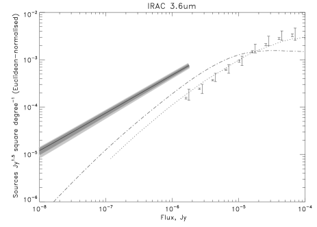
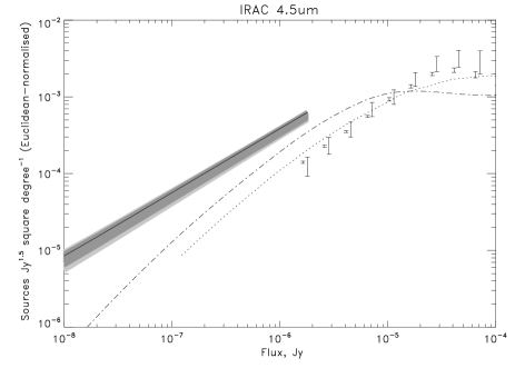
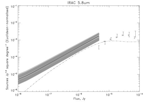
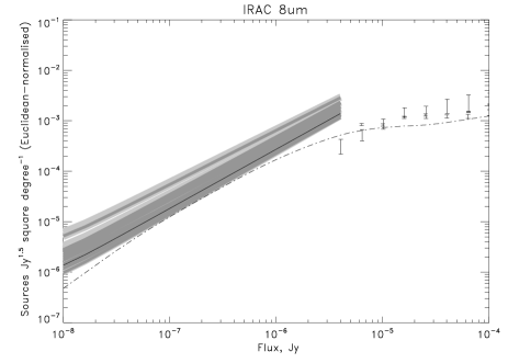
Figure 1: Plots of the fitted model number counts. In each case, the black line denotes the best-fit model, the grey regions are generated by plotting a sample of the MCMC models with the highest 68% and 95% posterior probability values, respectively. Note that all models are Euclidean normalised by multiplying by $flux^{2.5}$. The plotted points are actual number counts, measured by Fazio et al. (2004). Also plotted are model number count predictions due to Pearson (2005) (dot-dash line) and Franceschini et al. (2005) (dotted line).

Our aim is to extract statistical information about the nature of the faint galaxy population contributing to the confusion noise in the Spitzer GOODS survey. To achieve this, we will use a fluctuation analysis.

Fluctuation analyses uses the PDF of the data image pixels to constrain a parameterised model of the faint source number counts. The model is fitted to the data by comparing the PDF of the data image pixels with the corresponding PDF predicted for the chosen model. Various model-fitting techniques (in this case Markov-Chain Monte Carlo sampling) can then be used to determine the most likely set of parameter values for the model, given the data, as well as to determine the uncertainties on these estimates.

3.1 PDF estimation

In order to carry out a fluctuation analysis, we need a method of estimating the PDF of our data. The most straightforward way of doing this is to take a histogram of the image pixels, and this has several advantages.

Histograms are straightforward to implement and also to determine a reasonably ’optimal’ bin width (see e.g. Scott, 1992). It is also easy to construct a histogram such that the bins are essentially uncorrelated from one another, giving the individual bins Poissonian errors. Furthermore, for large numbers of pixels-per-bin, the errors tend towards Gaussianity, a feature that simplifies the calculation of likelihoods.

We note that there are a number of other possible choices of PDF estimators. In particular, fixed and adaptive kernel methods (see e.g. Vio et al., 1994) have become increasingly widely used in recent years. The superior performance of these methods comes at the price (in this context) of a more complicated error structure and greater computational requirements. We will therefore not consider them in this work.

3.2 Generation of model PDFs

Having estimated the PDF of our data, we need equivalent model PDFs to fit to it. In previous work, these have typically been generated from analytic solutions (see e.g. Condon, 1974). In this paper, however, we will adopt a slightly different approach, designed to more explicitly reflect the effects for which we must account.

Our method of determining model PDFs is essentially a Monte Carlo method, simulating a number of skies in order to find the required PDF. However, in order to speed up the calculation, we implement numerically-solved analytic solutions in order to determine the distribution of fluxes arising from any pixel on the sky (before the effect of the instrument point spread function), as well as the effect of instrumental noise.

Due to the nature of fluctuation analysis, we pay particular attention to dealing with the instrumental noise. The data used in this paper include pixel-by-pixel estimates of the noise variance. To properly account for variations in noise across the map, we generate the overall noise PDF by summing the Gaussian noise PDFs (characterised by said variances) for each pixel (and re-normalising). The noiseless model PDF is then convolved by this noise PDF and the resulting model PDF re-binned to match the histogram bins of the data PDF.

To test the robustness of our analyses to noise estimation, we ran test analyses in which we increased or decreased the noise variances by 20%. In all cases, the results were essentially unchanged, an outcome that is reasonable given that source confusion is the dominant effect in these observations.

We note that this method is all carried out on pixels of twice the resolution of the data we will be analysing. This matches the highest resolution publicly available point spread function for the IRAC instrument, allowing us to use all available information about the point spread function. The model resolution is halved by simple bin averaging after the point spread function convolution, but before convolution with the noise PDF.

3.3 Model-fitting, mapping the posterior probability distribution

For any analysis such as this, we are aiming to determine the most likely set of model parameters, given our data (and choice of model). From fundamental probability theory, we have Bayes theorem:

$$P(\theta|D,H)=\frac{P(D|\theta,H)P(\theta,H)}{P(D|H)}\,,$$ (1)

Where $P(\theta|D,H)$ is the posterior probability of the model parameters ($\theta$), given the data ($D$) and a hypothesis ($H$). $P(D|\theta,H)$ is the likelihood of the data given a set of model parameters, $P(\theta,H)$ represents any prior knowledge we may have and $P(D|H)$ is the Bayesian Evidence.

So, the posterior is the thing we want. Assuming uncorrelated, Gaussian errors on the PDF histogram bins, the (unnormalised) likelihood is given by the following equation.

$$L=exp(-{Q^{2}\over 2})$$ (2)

where $Q^{2}$ is given by

$$Q^{2}=\sum_{i=1}^{N_{bins}}\left({{d_{i}-m_{i}}\over\sigma_{i}}\right)^{2}$$ (3)

and $d_{i}$ is the number of data in the $i^{th}$ histogram bin, $m_{i}$ is the corresponding model value and $\sigma_{i}$ is the standard deviation associated with that histogram bin.

For this analysis, we choose uninformative flat priors, so that we are making minimal assumptions.

For the analyses presented in this paper, we will ignore the normalising Bayesian evidence term. However, we note that future work in this will undoubtedly benefit from using the evidence to compare the relative likelihood of different number count models being good descriptions of the data.

The information extracted by such an analysis is to be found in the posterior probability function. This function tells us, given our data (and any prior knowledge), the likely range of values of the model parameters. We wish therefore to map this function, in order to produce the results of our analysis.

The analysis methods we have described in the previous subsections allow us to determine the (unnormalised) posterior value for a given point in parameter space. By using some suitably efficient method of function mapping, we can hence obtain our results.

We will use Markov Chain Monte Carlo (MCMC) sampling (see e.g. Gilks et al., 1995) to do this. MCMC sampling is an efficient way of drawing a set of samples from the posterior probability distribution. It has a number of advantages over many more basic methods. Firstly, it returns not only the most likely solution, but also estimates of the uncertainties on all estimated parameters. Secondly, it estimates these uncertainties without needing to make any assumptions as to the functional form of the likelihood (such as are required by methods such as Fisher matrix analysis). The principal downside is that such an analysis can be computationally very expensive; typically $5\times 10^{4}$ to $10^{5}$ likelihood calculations are needed, several orders of magnitude more than most function maximisers.

In each of the four analyses we carry out, we use at least five MCMC chains, each 10,200 samples in length. We remove the first 2,000 samples from each case as they represent a ’burn-in’ phase, where the chains are moving towards the region of highest likelihood. This leaves us with over 40,000 samples for each analysis.

Ideally, we would want more samples than this (a typical rule-of-thumb for this type of analysis is $10^{5}$ or more samples), however we were limited in this work by the amount of time taken to compute the likelihood values; the analysis for each band took 3-4 weeks on a 3 GHz, dual-processor Linux box.

3.4 Choice of models

In this paper, we will fit the usual class of power law models for the differential source number counts, defined by the following equation.

$${dN\over dS}=\left\{\begin{array}[]{ll}N_{o}S^{-\delta}&(S>S_{cut})\\ 0&(S<S_{cut})\\ \end{array}\right.$$ (4)

The fitted parameters are $\delta$, $S_{cut}$ and $A$, where $A$ is given by the following equation.

$$A=\int_{0}^{S_{max}}{dN\over dS}dS$$ (5)

$S_{max}$ is chosen to exclude small numbers of bright sources at a level where the model will no longer be a fit to the observed number counts. We note that in each analysis we have removed regions of the data containing flux peaks bright enough to be due to sources brighter than the corresponding value of $S_{max}$.

The sources are assumed to be Poisson-distributed on the sky (i.e. we assume they are not clustered). We note that this model is strictly phenomenological. This approach, while not physically motivated, does produce constraints on the likely number count distribution of faint sources in the fields being analysed.

4 Analysis and results

Table 1: The results of fitting a one-power-law number count model to the data. For each band, the best-fit log-likelihood, number of histogram bins, best-fit mean source density, power law index, flux cut-off are given, along with the 95% confidence limits (determined from the 1D marginalised likelihood functions(see figure 4). Reduced chi-squared values are also given.

Band	Log(likelihood)	bins	source density ($10^{9}$ per sq. deg.)	index	cut-off ($10^{-12}$ Jy)	reduced chi-squared
3.6 microns	-162.7	98	1.62${}^{+0.62}_{-0.62}$	1.70${}^{+0.01}_{-0.05}$	15.0${}^{+8.5}_{-8.5}$	3.43
4.5 microns	-41.0	99	2.14${}^{+2.82}_{-1.24}$	1.67${}^{+0.02}_{-0.04}$	4.01${}^{+4.75}_{-2.70}$	0.86
5.8 microns	-54.1	98	1.44${}^{+1.82}_{-0.85}$	1.53${}^{+0.05}_{-0.03}$	0.24${}^{+1.37}_{-0.22}$	1.14
8.0 microns	-54.3	99	0.09${}^{+1.17}_{-0.03}$	1.33${}^{+0.14}_{-0.02}$	0.54${}^{+0.75}_{-0.53}$	1.13

Table 2: The integrated background light due to galaxy emission, for each of the four IRAC bands. These values are estimated in two parts. Faint is found analytically by integrating the best-fit model from our fluctuation analysis. Bright is the integrated light due to sources above the upper limit of our models and are taken from Fazio et al. (2004). The total is the sum of the previous two values. All errors shown are 95% confidence limits. Faint errors are determined from the 1D marginalised likelihood functions (see figure 6). Bright errors are not given in Fazio et al. (2004), so the total error is found by scaling those for Faint.

Band	faint ($10^{-9}wm^{-2}sr^{-1}$)	bright ($10^{-9}wm^{-2}sr^{-1}$)	total background ($10^{-9}wm^{-2}sr^{-1}$)
3.6 microns	5.23${}^{+0.31}_{-0.96}$	5.4	10.6${}^{+0.63}_{-1.95}$
4.5 microns	2.85${}^{+0.43}_{-0.48}$	3.5	6.4${}^{+0.97}_{-1.08}$
5.8 microns	1.79${}^{+0.56}_{-1.18}$	3.6	5.4${}^{+1.69}_{-3.56}$
8.0 microns	1.23${}^{+0.77}_{-0.74}$	2.6	3.8${}^{+2.38}_{-2.29}$

Figure 1 shows the results of our analyses. In each case, the solid black line denotes the best-fit model (whose parameters are given in Table 1). The shaded regions give the loci of 68% and 95% confidence regions, defined by taking the corresponding percentage of MCMC samples with the highest posterior probability values.

On each plot, the number counts determined for the four IRAC bands by Fazio et al. (2004) are plotted. The values plotted are those estimated for galaxy counts, with error bars denoting Poisson uncertainty. All values have been corrected for incompleteness using the estimates given in said paper. The plots also show the galaxy number count models of Pearson (2005) (dot-dash line).

In Figure 2, we re-plot the 3.6 micron number counts with a flux scaling of 0.75, in order to show the effect of a 25% (decrease) error in flux calibration.

Figure 3 shows the data PDFs estimated for each of the four IRAC bands (solid lines). Over-plotted (dashed lines) are the best-fit model PDFs determined from our analyses.

One of the great advantages of MCMC sampling is that it enables us to recover much information about the posterior probability distribution. Figure 4 shows the 1D, marginalised likelihoods for each of the three fitted parameters, for each of the four IRAC bands. For any set of samples drawn from the posterior distribution, marginalisation is straightforwardly achieved by taking a histogram of the samples over the parameter of interest.

The constrained faint number count models can be integrated to find estimates of their contribution to the the infra-red background light. Combining this with estimates of the contribution from bright sources taken from Fazio et al. (2004), we can thus obtain overall estimates of the integrated background light in the four IRAC bands. We note that for the purposes of these analyses, we cut off our number count models at the flux of the faintest Fazio et al point.

Figure 5 shows the proportion of the total background light resolved, as a function of flux. The result for the best-fit model is shown (black line); also plotted are a subset of the 68% (dark grey) and 95% (light grey) confidence region models, to indicate the statistical uncertainty in the results.

Figure 4 shows the marginalised 1D posterior probability distributions for the total integrated background light due to our constrained models (i.e. not including the contribution from brighter galaxies). These results are tabulated in table 2 and combined with the contribution from bright sources in order to provide estimates of the total background light due to galaxies in the four IRAC bands.

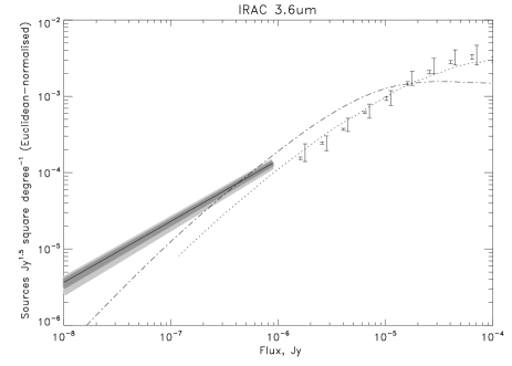
Figure 2: Plot of the fitted 3.6 micron model number counts, with model flux values scaled by $\times 0.5$, to simulate the effect of an error in flux calibration. (Note that this also affects the Euclidean normalisation). This shows that the difference between our results and the Fazio et al. (2004) number counts could be explained by a 50% relative difference in the flux calibration of the two sets of observations.

Figure 3: The pixel flux PDFs for the data (solid line) and the best-fit model (dashed line; partially obscured by solid line). The data PDF is estimated using a histogram of the image pixels from a given band. The model PDF is calculated using the method described in section 3. The overall noise PDFs are also plotted (dotted line). For ease of comparison, the noise PDFS are appropriately scaled and offset so that their peaks are coincident with the data PDFs.

Figure 4: The marginalised 1D posterior probability distributions for the fitted model parameters. The distributions generated by taking a histogram of the MCMC samples and are given in units of number of counts per bin. The level of structure in the distributions suggests that the MCMC chains have only borderline convergence (longer chains were not possible, due to computational constraints). This will not have a substantial impact on the broad results of this analysis.

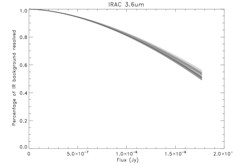
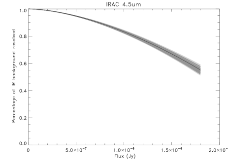
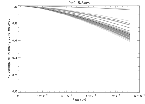
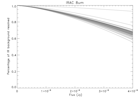
Figure 5: Estimates of the proportion of the IR background light that is resolved, as a function of flux. The proportion is calculated assuming that the ’total’ IR background light is given by values from Table 2. Shown are the best-fit solution (block line), along with a subset of the 68% (dark grey) and 95% (light grey) confidence region solutions.

Figure 6: The PDFs of the integrated background light due to the constrained number count models resulting from our analyses. These estimates do not include the contribution from brighter sources. The overall estimated contribution from all sources is given in Table 2.

5 Discussion and conclusions

Our analyses of the Spitzer GOODS HDF-N epoch one data have produced constraints on the faint source counts in the four IRAC bands (3.6, 4.5, 5.8, 8 microns). Fazio et al. (2004) estimate the contribution of stars to the counts at such faint fluxes to be be negligible. We therefore can regard the results in Figure 1 as approximating the faint galaxy counts in these bands. The analyses presented in this paper provide meaningful constraints on these differential number counts down to $10^{-8}Jy$, over two orders of magnitude fainter in flux than the faintest published number counts.

The plotted number count points in Figure 1 are the result of source extraction from other Spitzer observations, making them measurements that are independent of the data used in this paper. The most noteworthy discrepancy is that the fluctuation analyses seem to produce number counts that are systematically higher than those measured by Fazio et al. (2004). There are a number of possible explanations for this effect.

The first is suggested by Figure 2. A relative difference between the flux calibration of the data used in this paper and that of Fazio et al. (2004) could make the results consistent with one another.

Another possibility is that the number count model we have fitted is an over-simplification. Being strictly phenomenological, it would not be hugely surprising to find at least some deviations of this nature. Some non-power-law behaviour in the real faint number counts (for example, a plateau) could cause such an effect. Clustering of the real sources could also have an impact, as it is known that source clustering changes the expected fluctuation signal.

There is also the possibility of fluctuations from non-point-like sources, such as diffuse galactic emission. Fluctuation analysis is likely to be sensitive to such effects in the data, should they be present in substantial amounts.

Balanced against this is the goodness-of-fit of the models (see the reduced chi-squared values in Table 1). These show that in all cases except the 3.6 micron band, the fitted models are good representations of the data. Any statistically significant deviation of the real number counts from a power law would show up as an increase in the reduced chi-squared values.

The 3.6 micron data is fitted substantially more poorly by the model, so it is possible that we have detected non-power-law behaviour in this case. Indeed, we would expect the 3.6 micron data to be most sensitive to such deviations, as it has the lowest relative level of instrumental noise (see Figure 3) However, the fact that this over-estimate (relative to the Fazio counts) occurs in all four bands suggests that there is also something else occurring.

Other systematic effects in the Spitzer GOODS data may also play a part. Any non-Gaussianity in the noise could be significant, although the outlier rejection used to reduce the GOODS data guards against this. Issues such as the residuals present from flat-fielding may also have an impact, although if they add Gaussian noise, we have shown our analysis to be robust to this. We have also assumed a constant point spread function across the whole image, which may not be the case. Effects of this nature may contribute to an explanation of the observed discrepancy.

Similarly, there may be systematic effects present in the Fazio number counts. Faint source counts are, by their nature, very difficult to measure to high precision, especially when the issue of incompleteness is a factor (as it is here).

Although the data used in this paper has been background-subtracted, the possibility of some residual contamination from diffuse backgrounds such as galactic cirrus remains. The exact effect of this is unclear and it may be negligible. However, it may have some impact on our results.

Overall, it is clear that we expect some level of systematic uncertainty in addition to the more easily quantified random uncertainty. The level of consistency between the results from fluctuation analyses and direct source counting give us a crude measure of the level of these systematic uncertainties.

Figure 4 shows the 1D marginalised likelihoods for the fitted parameters. Each of these histograms is formed from at least 40,000 MCMC samples. This number is a little low for MCMC sampling analyses and this is reflected in some of the plots, where a degree of multiple peak structure can be seen. These features are more likely to represent imperfect convergence of the MCMC chains than any real feature, the result of the computational constraints on these analyses. Despite this, the broad results such as best-fit and confidence regions are still valid.

Figure 1 shows our results in comparison to the galaxy number count models of Pearson (2005) and Franceschini et al. (2005). Of particular note is the large excess of faint number counts in our results over those predicted the models. This result remains if the inconsistency between our results and the Fazio number counts is explained by a difference in flux calibration. If this is the case, this result indicates the presence of a significant amount of faint fluctuations in the IR background.

Constraint of the faint number counts allows us to estimate the contribution of faint galaxies to the integrated background light. One of the great advantages of MCMC analysis is that we can do this for each MCMC sample, thus correctly propagating the statistical uncertainty of our analyses to new quantities such as this. The plots in Figure 5 show that the Fazio counts reach a depth sufficient to resolve of order half of more of the integrated background light. The fluctuation analysis presented in this paper extends to fluxes over a factor of 100 fainter than this, therefore covering virtually all of the integrated background light in the four IRAC bands.

We have estimated the total integrated background light in each of the four IRAC bands (see Figure 4 and Table 2). The IRAC 3.6 micron band is comparable to the near-IR L-band (2.9 to 3.5 microns), for which there are several existing estimates of the integrated background light due to galaxies. In comparison to our 3.6 micron result of $10.6^{+0.63}_{-1.95}\times 10^{-9}wm^{-2}sr^{-1}$, Dwek & Arendt (1998) obtain $9.9\pm 2.9\times 10^{-9}wm^{-2}sr^{-1}$, Gorjian et al. (2000) obtain $11.0\pm 3.3\times 10^{-9}wm^{-2}sr^{-1}$, and Wright & Reese (2000) find $12.4\pm 3.2\times 10^{-9}wm^{-2}sr^{-1}$. We therefore conclude that our 3.6 micron results are consistent with all three of these L-band results. We also note that our errors are substantially smaller than for these measurements.

Also of interest are the results of Matsumoto et al. (2005), who measure the near-IR integrated background light using the Infra-Red Telescope in Space (IRTS). Their data extend from 1 to 4 microns. A representative measurement they obtain of the integrated background is (3.68 microns) $13.1\pm 3.7\times 10^{-9}wm^{-2}sr^{-1}$. On the basis of our 3.6 micron results, we therefore suggest that the longer wavelength results from Matsumoto et al. (2005) can be explained by the emission of faint, point-like objects, as seen in the Spitzer GOODS data. We note that this is consistent with the interpretations Matsumoto et al. (2005) have made using additional information from power spectra and colour information.

We also note the recent results of Kashlinsky et al. (2005), who detect an excess in the IRAC-band infra-red background, which they attribute to population III stars. While our analysis does not provide information to specifically comment on this interpretation, it is instructive to compare our findings. Kashlinsky et al. (2005) detect an excess in the infra-red background after subtracting a contribution from faint galaxies which they determine by extrapolating the Fazio et al. (2004) number counts using a fitted power law number count model. Our results likewise find a substantial excess over the extrapolated Fazio number counts. Furthermore, our results show a large excess over the faint number count model predictions shown in Figure 1. Even if this were in part due to calibration uncertainty, the differing power law slopes between our results and the models mean that some excess will remain (see, for example, Figure 2).

The analyses in this paper are subject to a number of caveats (which we have discussed above). We reach a number of conclusions (see below); these are all subject to the assumptions we have made in this analysis. Model-wise, We have assumed Gaussian instrumental noise (of known variance), a power law number count model over the range of interest, and that the sources are Poisson-distributed and point-like. Data-wise, we use the best available flux calibration and point spread function. We also assume that flat-fielding artifacts do not significantly bias our results. In conclusion, in this paper we present the following results.

1. Constraints on near-IR galaxy number counts. We use the Spitzer GOODS survey (HDF-N, data release one) to place constraints on the faint number counts in the four near-IR Spitzer IRAC wavebands. As the contribution due to stars at these fluxes is predicted to be small, these number counts approximate to galaxy number counts. We generate meaningful constraints on these number counts down to $10^{-8}Jy$, over two orders of magnitude fainter in flux than the deepest currently published number counts.

2. A discrepancy between our results and those of Fazio et al. (2004). Our results systematically overestimate the differential number counts with respect to the Fazio counts. We discuss a number of possible causes of this.

3. Determination of the background light due to unresolved point sources in each of the four IRAC bands. We estimate the proportion of background light dues to faint galaxies that is resolved, as a function of flux. We concur with the broad estimates of Fazio et al. (2004) that over half the background light is resolved by Spitzer into individual galaxies. We demonstrate that almost the entirety of the remaining integrated light is probed by our fluctuation analysis. We also estimate the contribution of faint galaxies to the integrated background light. By adding this to the estimate for bright sources given by Fazio et al. (2004), we obtain estimates of the total integrated background light. Our 3.6 micron result is found to be consistent with the L-band results of Dwek & Arendt (1998), Gorjian et al. (2000) and Wright & Reese (2000). This result is also consistent with the results from Matsumoto et al. (2005) at the corresponding wavelength. We note that our analyses do not impact on the substantial excess detected by Matsumoto et al. (2005) at shorter wavelengths.

4. Consistency with the recent detection of excess infra-red background reported by Kashlinsky et al. (2005). Although our analyses do not provide information of the interpretation of the Kashlinsky et al. (2005) result, we do detect a clear excess over the Fazio et al. (2004) number counts; the Kashlinsky et al. (2005) is also based on the existence of such an excess.

Fluctuation analyses are an invaluable way of probing galaxy number count distributions well below the confusion limit of any given instrument. Photometric surveys are now producing data sets where the statistical errors on such analyses are sub-dominant to the systematic uncertainties on such measurements. To improve the knowledge we can extract from fluctuation analyses, we must therefore pay particular attention to both understanding and accounting for the systematic influences on our data.

References

- Barcons et al. (1994) Barcons X., Raymont G. B., Warwick R. S., Fabian A. C., Mason K. O., McHardy I., Rowan-Robinson M., 1994, MNRAS, 268, 833
- Condon (1974) Condon J. J., 1974, ApJ, 188, 279
- Craig et al. (2004) Craig N., Mendez B. J., Wright E. L., 2004, American Astronomical Society Meeting Abstracts, 205,
- Dickinson & GOODS (2004) Dickinson M., GOODS 2004, American Astronomical Society Meeting Abstracts, 205,
- Dwek & Arendt (1998) Dwek E., Arendt R. G., 1998, ApJ, 508, L9
- Fazio et al. (2004) Fazio G. G., Ashby M. L. N., Barmby P., Hora J. L., Huang J.-S., Pahre M. A., Wang Z., Willner S. P., Arendt R. G., Moseley S. H., Brodwin M., Eisenhardt P., Stern D., Tollestrup E. V., Wright E. L., 2004, ApJS, 154, 39
- Fazio (2004) Fazio G. G. e. a., 2004, ApJS, 154, 10
- Franceschini et al. (2005) Franceschini A., et al., 2005, submitted
- Franceschini et al. (1993) Franceschini A., Martin-Mirones J. M., Danese L., de Zotti G., 1993, MNRAS, 264, 35
- Gilks et al. (1995) Gilks W. R., Richardson S., Spiegelhalter D. J., 1995, Marko Chain Monte Carlo in practice. Chapman & Hall, London
- Gorjian et al. (2000) Gorjian V., Wright E. L., Chary R. R., 2000, ApJ, 536, 550
- Kashlinsky et al. (2005) Kashlinsky A., Arendt R. G., Mather J., Moseley S. H., 2005, Nature, 438
- Matsumoto et al. (2005) Matsumoto T., Matsuura S., Murakami H., Tanaka M., Freund M., Lim M., Cohen M., Kawada M., Noda M., 2005, ApJ, 626, 31
- Nakagawa (2004) Nakagawa T., 2004, Advances in Space Research, 34, 645
- Oliver (1997) Oliver S. J. e. a., 1997, MNRAS, 289, 471
- Pearson (2005) Pearson C., 2005, MNRAS, 358, 1417
- Pearson et al. (2004) Pearson C. P., Shibai H., Matsumoto T., Murakami H., Nakagawa T., Kawada M., Onaka T., Matsuhara H., Kii T., Yamamura I., Takagi T., 2004, MNRAS, 347, 1113
- Pilbratt (2004) Pilbratt G. L., 2004, American Astronomical Society Meeting Abstracts, 204,
- Scheuer (1957) Scheuer P., 1957, Proc. Cambridge Phil. Soc., 53, 764
- Scheuer (1974) Scheuer P. A. G., 1974, MNRAS, 166, 329
- Scott (1992) Scott D. W., 1992, Multivariate Density Estimation. Multivariate Density Estimation, Wiley, New York, 1992
- Vio et al. (1994) Vio R., Fasano G., Lazzarin M., Lessi O., 1994, A&A, 289, 640
- Wall et al. (1982) Wall J. V., Scheuer P. A. G., Pauliny-Toth I. I. K., Witzel A., 1982, MNRAS, 198, 221
- Wright & Reese (2000) Wright E. L., Reese E. D., 2000, ApJ, 545, 43