Simulating the physical properties of dark matter and gas inside the cosmic web

Abstract

Using the results of a high-resolution, cosmological hydrodynamical re-simulation of a supercluster-like region we investigate the physical properties of the gas located along the filaments and bridges which constitute the so-called cosmic web. First we analyze the main characteristics of the density, temperature and velocity fields, which have quite different distributions, reflecting the complex dynamics of the structure formation process. Then we quantify the signals which originate from the matter in the filaments by considering different observables. Inside the cosmic web, we find that the halo density is about 10-14 times larger than cosmic mean; the bremsstrahlung X-ray surface brightness reaches at most $10^{-16}$ erg s^-1 cm^-2 arcmin^-2; the Compton-$y$ parameter due to the thermal Sunyaev-Zel’dovich effect is about $10^{-6}$; the reduced shear produced by the weak lensing effect is $\sim 0.01-0.02$. These results confirm the difficulty of an observational detection of the cosmic web. Finally we find that projection effects of the filamentary network can affect the estimates of the properties of single clusters, increasing their X-ray luminosity by less than 10 per cent and their central Compton-$y$ parameter by up to 30 per cent.

1 Introduction

In the standard picture of structure formation, the large scale structure observed in the spatial distribution of galaxies has evolved via gravitational instability from small perturbations present in the primordial cosmic density field. In particular, the later non-linear stages of this evolutionary process are thought to be responsible for the complex pattern of large voids surrounded by galaxies, clusters and superclusters exhibited by the observed galaxy distribution in modern catalogues, like the 2dF and SDSS surveys (see, e.g., Peacock et al., 2001; Tegmark et al., 2004).

This gravitational instability scenario has been largely confirmed by the perturbation theory in the weakly non-linear regime and by the results of numerical N-body simulations. In the cold dark matter (CDM) cosmological model, cosmic structures form by the accretion of smaller sub-units in a hierarchical bottom-up fashion. In this framework, galaxy clusters are of fundamental importance, since they are the largest bound systems in the universe and those most recently formed. Moreover, their abundances and spatial distribution retain the imprints of the underlying cosmological model; it is therefore possible to constrain the fundamental parameters of the model by studying the cluster properties and their redshift evolution (see Rosati et al., 2002; Voit, 2005, and references therein).

Still, the theoretical picture emerging from numerical simulations is even more intriguing. The largest dark matter haloes, which are expected to host the richest galaxy clusters, seem to be preferentially located at the intersections of one-dimensional, filamentary structures having a much smaller density contrast of the order of unity. From a dynamical point of view, this network of filaments (the so-called cosmic web) represents the preferential directions along which the matter streams to build the massive and dense structures located at the nodes. This picture, first emerged from N-body experiments, was lately understood in a theoretical framework (see Bond et al., 1996), in which the cosmic web corresponds to the density enhancements present in the primordial field that are then sharpened by the following non-linear evolution (see also Doroshkevich et al., 1982). A firm prediction of this model is that filaments represent bridges between denser spots identified with galaxy clusters.

The observational confirmation of this general picture resulted to be challenging. Some evidence arose from the presence of elongated structures such as the Great Wall (Geller & Huchra, 1989), in the galaxy spatial distribution, and from the tendency of neighboring clusters to be aligned (see, e.g. Plionis et al., 2003). More recent attempts at detecting filaments which make use of specific statistical analyses of modern galaxy surveys gave new support for the existence of the cosmic web (see, e.g., Bardelli et al., 2000; Ebeling et al., 2004; Pimbblet & Drinkwater, 2004; Pimbblet et al., 2004; Bharadwaj & Pandey, 2004; Pimbblet, 2005; Porter & Raychaudhury, 2005; Pandey & Bharadwaj, 2005). Further evidence has been found by studying the ultraviolet absorption line properties of active galactic nuclei projected behind superclusters of galaxies (Bregman et al., 2004).

Hydrodynamical simulations, including the treatment of the gas component, suggest that regions of moderate overdensity like filaments host a significant fraction of gas with a temperature between $10^{5}$ and $10^{7}$ K, the so-called warm-hot intergalactic medium (WHIM) (see, e.g. Cen & Ostriker, 1999; Pierre et al., 2000; Croft et al., 2001; Davé et al., 2001; Phillips et al., 2001). This gas may reveal its presence through its bremsstrahlung emission in the soft X-ray band. However, the expected signal appears too small to be clearly detected by the present generation of satellites: in the literature there are only a few claims of possible detections of WHIM emission (Scharf et al., 2000; Zappacosta et al., 2002; Markevitch et al., 2003; Kaastra et al., 2003; Finoguenov et al., 2003).

Much effort has been put into investigating the overall contribution of diffuse gas to the soft X-ray background (see, e.g. Croft et al., 2001; Roncarelli et al., 2006). A major issue is to distinguish it from that of the two dominant sources, i.e. the active galactic nuclei and the hot gas in our own Galaxy. Thanks to deep observations with the Chandra satellite (Brandt et al., 2001; Rosati et al., 2002; Bauer et al., 2004; Worsley et al., 2005), it has become clear that at least 90 per cent of the background in the (0.5-2 keV) band is contributed by discrete sources, thus implying an upper limit to the WHIM contribution. This result can be used to constrain the thermal properties of baryons and their cosmic history, providing important information on the evolution of galaxy clusters (see, e.g., Voit & Bryan, 2001; Bryan & Voit, 2001a; Xue & Wu, 2003).

An alternative way to investigate the diffuse baryons in filaments is the Sunyaev-Zel’dovich (SZ) effect (see, e.g., the simulated maps obtained by da Silva et al., 2001; Springel et al., 2001; White et al., 2002). The SZ and bremsstrahlung signals have a different dependence on the gas density and thus can be used to investigate the gas properties in two different but complementary environments. An additional probe of the WHIM at intermediate angular scales and redshifts is enabled by the study of the cross-correlation between soft X-ray and SZ maps, like those which will be obtained by planned missions in the future (Cheng et al., 2004).

Finally, gravitational lensing represents a unique tool for constraining the mass distribution of the cosmic structures. On galaxy cluster scales, strong gravitational lensing is used for measuring the mass in the inner regions of the lenses, where highly distorted images of background galaxies appear in form of arcs. In the outer regions of clusters, where the surface density is smaller, the gravitational lensing effects manifest themselves as small changes of the source shapes and orientations, which can be detected only by averaging over a large number of galaxies in a finite region of the sky. Due to the intrinsic ellipticities of the background galaxies, the weak lensing approach is unfortunately limited by noise but still represents a powerful method for reconstructing the lens mass distribution. Compared to other techniques, which make use of the light for tracing the mass, the largest advantage comes from the fact that it is model-independent and that no strong assumptions are required when converting the lensing signal into a mass measurement. Although this method has worked successfully in reconstructing the mass distribution around many galaxy clusters, it has failed yet to detect shallow surface density structures like the cosmic web. It is expected that the typical surface mass density along the filament is too small for producing a weak lensing signal detectable with the current instruments (Jain et al., 2000). However, as suggested by Dietrich et al. (2005), the effect might be measurable if the clusters connected by the filament are nearby. A few candidates of filaments have been found through weak lensing so far, but without strong constraints. There is some evidence of a bridge connecting member clusters in the Abell 901/902 (Gray et al., 2002) and MS0302+17 (Kaiser et al., 1998; Gavazzi et al., 2004) superclusters. Dietrich et al. (2005) recently claimed the detection (at the $2\sigma$ level) of a filamentary structure between the two massive clusters A222 and A223. Their result is also supported by the good correlation with the optical and X-ray data. Recently, Porter & Raychaudhury (2005) identify two major filaments in the Pisces-Cetus supercluster at the edges of the 2dF Galaxy Redshift Survey and the Sloan Digital Sky survey.

Although, many observations of filamentary structures have been attempted using a variety of techniques, as described earlier, it is still unclear how such filaments may appear in many of their observables. This makes it difficult to compare different observations, mainly because they may be efficient in probing different constituents of the cosmic web. The main goal of this paper is to cover this gap to give a detailed overview of how filamentary structures look like from as many points of view as it is possible. We focus our attention on a restricted region of a cosmological simulation, which contains a supercluster-like structure extending over several Mpc. We perform a new high-resolution hydrodynamical simulation of this sub-volume, which represents one of the largest overdensities found in the original cosmological box. The region contains four galaxy clusters with a mass larger than about $10^{15}M_{\odot}$, connected by filaments and bridges. We discuss the properties of these structures with respect to many observables.

The plan of the paper is as follows. In Section 2 we describe the general characteristics of the simulation used in the following analysis. In Section 3 we introduce the concept of cosmic web and bridges, discussing their morphological appearance. Section 4 is devoted to the discussion of the main properties of the gas inside the bridges: in more detail we analyze its density, temperature and velocity field. In Section 5 we discuss the observational implications of the previous results: in particular we study the density and spatial distribution of haloes, the characteristics of the bremsstrahlung emission in the X-ray band, the Compton-$y$ parameter produced by the thermal SZ effect, and the weak gravitational lensing signal. Finally, we summarize our results and draw our main conclusions in Section 6.

2 The numerical simulation

The numerical simulation discussed in this paper follows the formation and evolution of a supercluster-like structure, which at the present epoch contains 27 haloes with virial mass $M_{\rm vir}$ larger than $0.7\times 10^{14}M_{\odot}$. Four of them are massive galaxy clusters with $M_{\rm vir}\raise-2.0pt\hbox{\hbox to0.0pt{\hbox{$\sim$}\hss}\raise 5.0pt\hbox{$>$}\ }10^{15}M_{\odot}$, connected by bridges and sheets of gas and dark matter. This overdense region was suitably chosen in the final output of a parent cosmological N-body simulation (Yoshida et al., 2001; Jenkins et al., 2001), which follows the evolution of the dark matter (DM) component only in a box with size $479\,h^{-1}$Mpc comoving; the assumed background cosmology is the standard ‘concordance’ cosmogony, i.e. a flat $\Lambda$CDM model with a present matter density parameter $\Omega_{\rm 0m}=0.3$, a present baryon density parameter $\Omega_{\rm 0b}=0.04$, a Hubble parameter $h=0.7$, and a power spectrum normalization corresponding to $\sigma_{8}=0.9$.

By adopting the ‘Zoomed Initial Conditions’ (ZIC) technique (Tormen et al., 1997), the corresponding Lagrangian region in the initial conditions was resampled to higher resolution by appropriately adding small-scale power and increasing the number of particles. This allows the mass and force resolution to be increased almost at will. In order to reproduce the global tidal field, outside the high-resolution (HR) region the primordial fluctuations are still sampled, but with a reduced number of particles having larger mass. The exact shape of the HR region has to be accurately selected to avoid any contaminating effect from these low-resolution (LR) particles. This was done using an iterative process as follows. Starting from a first guess of the HR region, we run a LR DM-only re-simulation. Analyzing its final output, we individuate in the initial conditions the Lagrangian region containing all the particles that are at a distance smaller than 5 virial radii ($R_{\rm vir}$) from at least one of the 27 main haloes. Applying ZIC, we generate new HR initial conditions and run one more DM-only re-simulation. The procedure is iteratively repeated until we find that none of the LR particles enter the HR region, which would be possible because of the introduction of small-scale modes. Because of the complex geometry of the supercluster region considered, in our case this procedure required more than 20 low-resolution DM-only re-simulations. The final HR region has an irregular shape which can be contained into a box of roughly $50\times 50\times 70$ Mpc³. All 27 haloes are free from contaminating boundary effects up to at least 5 times $R_{\rm vir}$. These new initial conditions were then adapted for our hydrodynamical run, performed using GADGET-2 (Springel, 2005), a new version of the parallel TreeSPH code GADGET (Springel et al., 2001), which adopts an entropy-conserving formulation of SPH (Springel & Hernquist, 2002). Gas particles have been introduced only in the HR region by splitting each original particle into a gas and a DM particle with masses $m_{\rm DM}=1.61\times 10^{9}\,M_{\odot}$ and $m_{\rm gas}=2.43\times 10^{8}\,M_{\odot}$, respectively. The Plummer–equivalent gravitational softening was set to $\epsilon_{\rm Pl}\approx 7$ kpc comoving from $z=2$ to $z=0$, while it was taken to be fixed in physical units at higher redshifts. Our re-simulation, which includes non-radiative hydrodynamics only, was performed in parallel by using approximately 13,000 hours on 16 CPUs on an IBM-SP4 located at the CINECA Supercomputing Centre in Bologna, Italy.

Finally, let us to remark that the most important difficulty in creating the suitable initial conditions and in running the simulation has been the fact that the structure we want to study, i.e. the cosmic web, is quite extended and has very low density. Consequently a HR simulation needs to follow a large volume with a very large number of particles: in the HR region we used approximately $1.4\times 10^{7}$ gas particles and $1.7\times 10^{7}$ DM particles, plus $1.4\times 10^{6}$ LR particles in the external region.

3 The cosmic web

The distribution of dark matter and gas inside the simulated supercluster region is quite complex. This is already evident in Fig. 1, where we present projected maps obtained from the results of the final output of the simulation, corresponding to redshift $z=0$. Only in the left column we displayed the whole HR region (i.e. $50\times 50\times 70$ Mpc³) to give a better impression how the supercluster is embedded within its environment. In the other columns and also in the following analysis we restrict ourself to a zoom of the high-resolution region (ZHR) of dimensions $30\times 30\times 50$ Mpc³. This sub-box contains all the filaments connecting the four main halos within the supercluster region. The different rows correspond to the three different cartesian projections. In the left column, each dot represents a halo containing at least 30 (DM+gas) particles, i.e. with a mass larger than about $5\times 10^{10}\,M_{\odot}$. In the same plots the circles show the positions (and virial radii) of the four most massive galaxy clusters belonging to the supercluster, which are identified by the letters A to D, starting from the most massive object. In Table 1 we summarize the main properties of these four clusters computed inside the virial radius, $R_{\rm vir}$ (defined by using the overdensity threshold dictated by the spherical top-hat model; see e.g. Eke et al. 1996): the virial mass, $M_{\rm vir}$; the mass-weighted temperature, $T_{\rm MW}$; the X-ray luminosity computed in the [0.1-10 keV] energy band, ($L_{\rm X}$); the central value of the Compton-$y$ parameter produced by the SZ effect (averaged over the three different Cartesian projections). Each of these four objects is very well resolved containing inside the virial radius between $1\times 10^{6}$ and $2\times 10^{6}$ particles, depending on their mass. The methods applied to compute the last two ‘observables’ will be briefly described in the following Sect. 5. Notice that in this paper we prefer to use the mass-weighted estimator of the temperature because it is more related to the energetics involved in the process of structure formation. As shown in earlier papers (Mathiesen & Evrard, 2001; Mazzotta et al., 2004; Gardini et al., 2004; Rasia et al., 2005), the application of the emission-weighted temperature, even if it was originally introduced to extract from hydrodynamical simulations values directly comparable to the observational spectroscopic measurements, introduces systematic biases when the structures are thermally complex, such as in the supercluster region considered here.

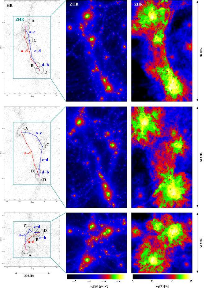
Figure 1: Projected maps extracted from the simulation. Left column: the distribution of the haloes containing at least 30 (DM+gas) particles, extracted from a box of size $50\times 50\times 70$ Mpc³ placed within the HR region. Circles indicate the positions and the virial radii of the four most massive objects (labeled from $A$ to $D$), while the lines refer to the paths used to follow the filamentary structures. The rectangle shows a zoom into the HR region (ZHR, with size $30\times 30\times 50$ Mpc³) displayed in the other colums, which has no contamination effects produced by the presence of LR particles. Central column: the projected gas density in a logarithmic colour scale (shown at the bottom). Right column: the projected mass-weighted temperature, also in a logarithmic colour scale shown at the bottom. Each row refers to a different cartesian projection: from top to bottom the projection is along the $z$, $x$ and $y$ axes.

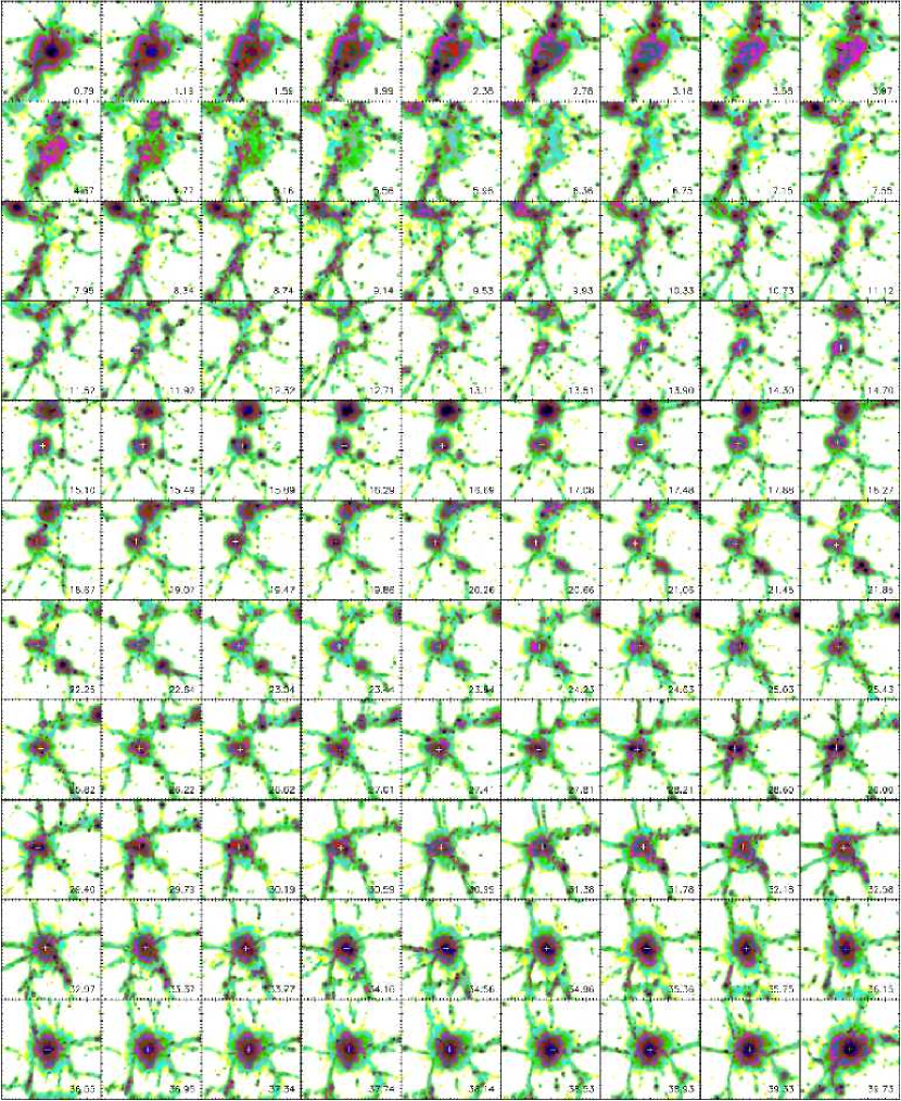
Figure 2: Contours for gas isodensity levels computed in 100 equidistant slices located between haloes $A$ and $B$. The number at the bottom right corner indicates the distance (in Mpc) from halo $A$. The white cross marks the centre of the filament and it has been shown only for the slices for which the symmetry axis of the filament is roughly parallel to the line of sight. Notice that this does not occur in the slices with distances between $0.79$ and $11.52$ Mpc from cluster $A$. The color scale is the same than in the upper panels of Figure 3.

Table 1: The main properties of the four largest haloes found inside the supercluster region. Column 1: the halo identification letter. Column 2: the virial radius $R_{\rm vir}$ (in units of Mpc). Column 3: the virial mass $M_{\rm vir}$ (in units of $10^{15}M_{\odot}$). Column 4: the mass-weighted temperature $T_{\rm MW}$ (in units of keV). Column 5: the X-ray luminosity, $L_{\rm X}$, computed in the [0.1-10 keV] energy band (in units of $10^{45}$ erg s^-1). Column 6: the central value of the Compton-$y$ parameter, averaged over the three cartesian projections (in units of $10^{-4}$).

Halo	$R_{\rm vir}$	$M_{\rm vir}$	$T_{\rm MW}$	$L_{\rm X}$	$y$
identification	(Mpc)	($10^{15}M_{\odot}$)	($10^{8}$K)	($10^{45}$ erg s-1)	($10^{-4}$)
$A$	3.25	1.89	0.69	2.08	1.82
$B$	3.18	1.79	0.70	1.33	1.37
$C$	2.78	1.19	0.46	1.26	1.04
$D$	2.58	0.95	0.55	1.42	1.59

The panels in the central and right columns of Fig. 1 are the projected maps for the gas density and mass-weighted temperature, respectively. In these cases the displayed region (ZHR) corresponds to the rectangles marked in the panels on the left. From the gas distribution, it is easy to recognize the positions of the four massive clusters, where the projected density can be larger than $10^{-2}$ g cm^-2. At the same locations, also the temperature maps have the highest values, with $T\geq 5\times 10^{7}$ K. In all projections than the thermal structures of the clusters named $B$ and $D$ appear as overlapping because of their small projected distance.

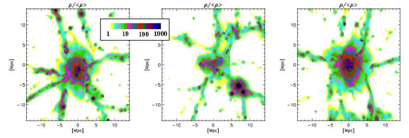
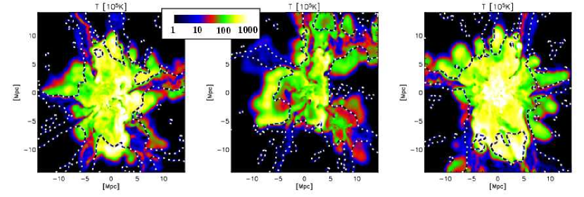
Figure 3: Upper panels: contours for gas isodensity levels computed on a plane which is located half-way between different cluster pairs and orthogonal to the bridge direction. Different panels refer to the bridges connecting clusters $A$ and $C$ (left), $B$ and $C$ (centre) and $B$ and $D$ (right). The logarithmic colour scale (in units of the mean density) is also reported. The side length of the displayed regions corresponds to 30 Mpc. Lower panels: the same but for gas (mass-weighted) temperature (in units of $10^{5}$ K). For reference, the dashed lines show the gas isodensity contour level corresponding to unity, already displayed in the upper panels.

Looking at the distributions of both haloes and gas, the presence of the so-called cosmic web is evident, i.e. elongated structures (one- or two-dimensional bridges) connecting the main virialized structures and spanning the whole region. Along these structures we find that the gas temperature, the 3D density and the projected density are typically much lower than $10^{7}$ K, $10^{-28}$ g cm^-3 and $10^{-3}$ g cm^-2, respectively.

As discussed in detail by Colberg et al. (2005) who analyzed a set of 228 filaments identified in a high-resolution N-body simulation for a $\Lambda$CDM cosmology, it is not easy to define a shape for this kind of structures. They found that roughly half of the filaments are either warped or lie off the line connecting two galaxy clusters. This is confirmed also in our simulation. In the left column of Fig. 1 the paths along which we measure some of the properties of the filamentary structures, namely the bridge connecting the clusters $A$, $B$ and $D$, and the bridge connecting the clusters $A$, $C$ and $B$, are indicated by lines. The paths are found iteratively. Firstly, we define a straight line connecting the cluster pairs; then, we cut a slice perpendicular to this line and find the maximum of the gas density on the slice. We repeat the same procedure iteratively, by cutting other slices in between the newly defined connecting points. The search for new points stops when the positions of the gas density maxima in two consecutive slices converge within the resolution limit. The path lines appear to be not perfectly aligned along the cluster-cluster axis, with the exception of the path between clusters $B$ and $D$, the closest pair, which has a straight structure. In general, by analyzing the several bridges present in the simulation it seems that a typical coherence length for the direction of these structures is about $\sim 5$ Mpc, but it can reach even higher values, as shown in the example in Fig. 2, where we present a tomography of the 40 Mpc wide region between haloes $A$ and $B$, made by using 100 equidistant slices. From the plots it is clear that the filament departs from halo $A$ in the lower left corner. At distances larger than 10 Mpc the elongated structure starts to bend in the direction of halo $B$. Then, it stays approximately parallel to the axis joining the two haloes for more than 25 Mpc, before it merges with cluster $B$. In different panels of the tomography it is evident that the filament represents a junction of several sheets present in the cosmic web. Although the position of the structures changes along the filament, the tomography clearly shows that the basic properties of the filament itself are quite stable for very large distances. This is particularly evident along the last 25 Mpc, where the slices of the tomography are roughly orthogonal with respect to the filament: the extension of the filament (roughly 5 Mpc in radius), as well as the position and number of sheets entering it do not vary in a significant way.

The matter bridges present in the projected maps shown in Figs. 1 and 2 can correspond both to two-dimensional (sheets) and one-dimensional (filaments) structures. These structures have been already studied in previous detailed analyses of numerical simulations: the results show that in many cases the filamentary structures are quite complex systems, not always well defined in one dimension, but often corresponding to projected sheets or intersections of them (Dave et al., 1997; Sathyaprakash et al., 1998; Colberg et al., 1999; Pierre et al., 2000). In order to better understand the true shape of the structures defining the cosmic web, in the upper panels of Fig. 3 we show for three different bridges between clusters the density distribution of the gas computed on a plane which is orthogonal to the bridge direction and which is located half-way between the two clusters defining it. The bridge A-C (left panel) appears to be very irregular, with the presence of different matter chains entering the central structure. The bridge C-B (central panel) can be very well described as the intersection of several sheets. Finally, the bridge connecting the clusters $B$ and $D$ (right panel), is more regular and corresponds to a higher gas overdensity because the two systems are very close and expected to merge in the near future.

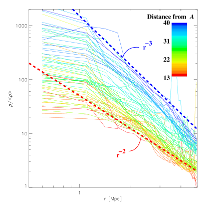
Figure 4: The radial gas density profiles in the filamentary structure connecting haloes $A$ and $B$ (see Fig. 2), as a function of the distance from the filament centre. Different coloured curves refer to slices located at different distances $d$ from cluster $A$ (see the corresponding colour bar); only results for slices with $d>13$ Mpc are shown. The red and blue dashed lines show the asymptotic trends, $r^{-2}$ and $r^{-3}$, respectively

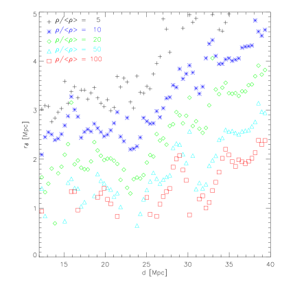
Figure 5: The measured thickness $r_{\delta}$ of the filament shown in Fig. 2, as function of distance $d$ from halo $A$. The results are shown for different overdensities, as indicated in the plot.

Taking advantage of the extension and regularity of the filament connecting haloes $A$ and $B$, we can measure its radial gas density profile as a function of the distance from cluster $A$. This quantity has been plotted in Fig. 4 for all the slides shown in Fig.2 having a distance larger than $\approx 13$ Mpc from the cluster A. Each profile is drawn up to 5 Mpc, which represents the typical scale up to which the filament looks round, and a radial profile can be safely defined: at larger distances the structure dissolves into sheets of matter, developing the arm-like structures visible in several slices. In the plot the density profiles are coloured according to their position along the filament (see the colour bar). It is clear that the profiles grow when moving towards the cluster B, reaching the highest value for the slide centered on the cluster. In this case the gas profile falls off as $r^{-3}$ (dashed-thick blue line) in the outer part, as expected from a Navarro-Frenk-White profile (Navarro et al., 1997): this confirms that the gas behaves as the dark matter component in the external part. On the other hand, the profiles computed along the filament (red and green lines) seem to be less steep: for example, in the slice located at a distance of about $13$ Mpc from the cluster $A$, they decrease in the external part like $r^{-2}$ (dashed thick red line). Also the slopes of the density profiles in the inner part seem to be shallower along the filament than in proximity to the clusters. Notice that the transition between the two regimes occurs at distances which exceed by almost a factor of four the virial radius of cluster $B$.

The previous result is confirmed by the analysis of the thickness of the filament, $r_{\delta}$, defined as the radius at which the profiles drop below a given density threshold. In Fig. 5 we show the behaviour of $r_{\delta}$, as a function of the distance $d$ from $A$. Even if there are some fluctuations produced local substructures, it is evident that the thickness is roughly constant up to $d\approx 30$ Mpc, then it monotonically increases when approaching the cluster $B$. Notice that this rise starts at a large distance (larger than 10 Mpc) from the halo. This result is independent of the chosen density threshold.

4 Properties of the gas inside the bridges

We now discuss the physical state of the gas contained inside the bridges. This is relevant to understand how the filaments and the sheets can be seen in the optical, X-ray and millimetric bands (see the next section). We estimate the gas properties making use of the SPH kernel to interpolate their value at different positions along the filamentary paths drawn in the left panels of Fig. 1. The results for the structures connecting galaxy clusters $A$, $B$ and $D$ and galaxy clusters $A$, $C$ and $B$ are shown in Fig. 6 (left and right panels, respectively).

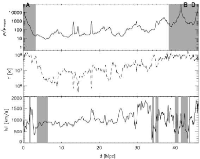
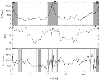
Figure 6: The physical state of the gas along the bridges connecting the galaxy clusters: the paths A-B-D and A-C-B (see for reference the left panels in Fig. 1) are shown on the left and right, respectively. Upper panels: the gas density (in units of the mean density); the grey regions correspond to the virial radii of different clusters (as labeled by the letters); notice that clusters B and D are so close that their radii appear as overlapped. Central panels: the gas (mass-weighted) temperature (in units of K). Bottom panels: the modulus of the three-dimensional velocity field (in units of km/s); the grey regions indicate where the velocity field is well aligned with the filamentary structure, i.e. where it forms an angle smaller than 45 degrees with the axis of the filament.

¿From the curves showing the behaviour of the gas density along the filaments (top panels), the positions of the largest galaxy clusters are clearly identifiable, as well as their profiles declining towards their virial radii. In the bridges between them, the gas density stays relatively constant, with typical values between 10 and 100 times the mean (baryonic) density. Some spikes are found, which are produced by smaller structures, where the gas density is larger. The corresponding masses are of the order of the galaxy masses.

More interesting is the trend shown by the mass-weighted temperature (central panels). The highest values obviously correspond to the clusters, with evidence in some cases of a decrement (by a factor 2) towards the virial radius (see also Bryan & Norman, 1998; Thomas et al., 2001; Borgani et al., 2004; Rasia et al., 2004). In other cases (see the close pair formed by clusters $B$ and $D$ or the regions surrounding the clusters $A$, $C$ and $B$ in the right panel) the outward movement of the accretion shocks creates extended, almost isothermal regions (with $T_{\rm MW}>5\times 10^{7}$ K). A temperature rise corresponding to about two orders of magnitude is located at distances larger than 2 virial radii. The minimum value in the bridges is around $10^{6}$ K. We notice also that in correspondence of the small structures present in the bridge $A$, $B$, $D$ (shown on the left) $T_{\rm MW}$ is smaller than in the surrounding regions: this is due to the fact that these objects formed before being heated by the accretion shocks of the larger structures.

Finally, we show in the lower panels the velocity field along the bridges. The displayed quantity is the modulus of the three-dimensional field, which reaches values larger than 1000 km/s. The shaded regions indicate where the infall direction of the gas forms an angle of less than $45$ degrees with the axis of the filament. The velocity field tends to be aligned to the direction of the filamentary structure close to the virial radius of the clusters. This evidences that the gas is flowing towards the clusters along the bridges. On the contrary, half way between the dominant clusters the motion tends to be orthogonal to the filaments, suggesting that they have a net motion with respect to the box.

The complexity of the thermal structure in the bridges is more clearly evident in lower panels of Fig. 3, where we show the iso-temperature levels as computed on the same planes shown in the corresponding upper panels. We find large and sharp gradients in the temperature structure positioned far from the centre of the bridge. Again, there is a strong correlation between the features present in the thermal distribution and those in the gas density. This is an indication that at $z=0$ the accretion shocks moved out of bridge, heating also regions at lower density. This process tends to create an extended smooth isothermal region, as more evident in the right panel, where the smaller distance between the two dominant clusters $B$ and $D$ speeds up the mechanism. Since the temperatures reached in this shock-heating process can be as large as $10^{7}$ K, it would be possible that non-negligible effects can be produced on the observational quantities, as it will be discussed in the next section.

Finally it is quite interesting to quantify the density and temperature distributions for the gas inside the bridges and compare them to the corresponding results in more typical regions. At this aim we define bridges as cylindrical regions connecting pairs of galaxy clusters, starting outside $R_{\rm vir}$ and having a radius of 5 Mpc. In particular we consider the two bridges between clusters A and C, and between clusters C and B. As examples of different “typical regions” we consider (i) the distributions computed in the whole ZHR region; (ii) a box of 70 Mpc³ extracted from a different hydrodynamic simulations which was performed using the same numerical code (assuming the same non-radiative gas-physics and the same cosmological model). The initial conditions have been constrained in a way, that the final large scale structure at $z=0$ is representing the observed Local Universe (LU), with the position of the Milky Way in the origin. The mass resolution is slightly smaller than that of ZHR (by a factor of 2.7), but this is not relevant for this comparison. More details on the LU simulation can be found in Dolag et al. (2005). The results for the density and temperature distributions are presented in Fig. 7 (left and right panels, respectively). The decreasing (increasing) curves in the upper panels show the volume fractions having density or temperature larger (smaller) than a given threshold, while in lower panels we present the same quantities, but in terms of mass fraction.

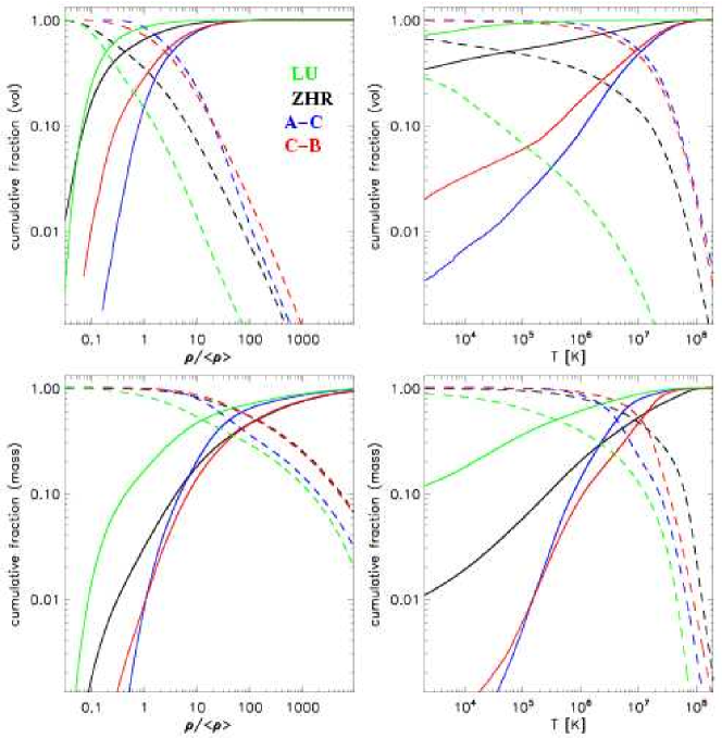
Figure 7: Left panels: the increasing solid (decreasing dashed) curves represent the cumulative fraction of volume (upper panel) or mass (lower panel) with a gas density smaller (larger) than a given value. Different lines refer to different regions in our simulation: the ZHR box, the bridges A-C and C-B are shown by black, blue and red lines, respectively. For comparison we also show the results obtained from a different simulation representing a (70 Mpc)³ box in the Local Universe (LU), centred at the Milky Way position (green lines). Right panels: the same as in the left panels, but for the gas temperature distribution.

Analysing the gas distributions (left panels), we find that the gas properties in the two bridges A-C and C-B are not very different: for both 80-90 per cent of the volume and $\approx 99$ of the mass have a density larger than the mean value, while approximately 20 per cent in volume and 80 per cent in mass corresponds to an overdensity of $\rho/\langle\rho\rangle>10$. The different morphology of the bridges (A-C appears very irregular, while C-B is an intersection of several sheets; see Fig. 3 and the corresponding discussion in the previous section) influences the high-density tail: in fact the bridge C-B displays slightly larger fractions of volume and mass at overdensity larger than 1000, with respect to the bridge A-C. As expected, the two filamentary structures represent regions at high density when compared to the whole ZHR region, which also includes extended underdense volumes (about 70 per cent has $\rho/\langle\rho\rangle<1$). The differences with respect to the LU simulation are even larger: in fact it is well know that our Milky Way is embedded in a slightly underdense region and this is reflected in the density distributions. The same trend is found considering the mass fraction, where however the inclusion of large virialized objects in the ZHR region and in the LU box enhances the probability of having gas mass at high density, reducing the differences with respect to the bridges.

Similar considerations can be done looking to the temperature distributions (right panels). The thermal structure inside the bridges is similar, with half of the volume occupied by gas at $T>10^{7}$ K. This fraction is much larger than that the corresponding results in the ZHR region (about 10 per cent) and in the LU simulation (less than 1 per cent). The same trend is evident for the volume-weighted mean temperature: about $10^{7}$ K for the bridges, about $10^{5}$ K in the ZHR region and less than $10^{3}$ K in the LU simulation. This is again an effect due to the presence in the two last cases of extended low-density regions, which occupy large volumes and are at low temperatures. In fact, considering the mass-weighted fractions, the differences between the bridges and the ZHR and LU regions are reduced: the mean mass-weighted temperature are approximately $2\times 10^{7}$, $10^{7}$, $5\times 10^{6}$ and $3\times 10^{5}$ K, for bridge C-B, ZHR region, bridge A-C and LU simulation, respectively. In this case, the difference between the two bridges can be again related to their different morphology: the sheet intersections for bridge C-B increase the fraction of gas particles at high density and consequently their temperature, making it on average denser and hotter than bridge A-C and ZHR region.

Finally, it is also important to investigate the gas properties in connection with the WHIM, which is well know to be preferentially located in the filamentary structures constituting the cosmic web. If we define the WHIM as the gas having a temperature ranging from $10^{5}$ and $10^{7}$ K, we find that it represents 22 and 77 per cent of the mass contained in the bridges C-B and A-C, respectively. The large difference between the two bridges is again produced by their different morphology. From the other side the percentage of mass corresponding to the WHIM is of order of 50 per cent in both HR region and LU simulation. In terms of spatial distribution, the WHIM occupies 37 per cent of the volume in both bridges, 33 per cent in the whole ZHR region and only 6 per cent in LU region.

5 Observables

In this section we will give an overview over several observables which are related to the gas and to the dark matter contained in the bridges. In particular we will discuss the properties of the halo distribution, the emission in the X-ray band, the thermal SZ effect and weak gravitational lensing.

5.1 Halo distribution

A first possible way to identify the matter present in the filamentary structures is to directly investigate the galaxy distribution in extended redshift surveys. The detailed study of specific regions of the universe, like those between close pairs of galaxy clusters, gave increasing support to the web-like vision of the universe (see, e.g., Pimbblet & Drinkwater 2004; Pimbblet et al. 2004; Ebeling et al. 2004), also suggested by wedge diagrams of the large scale structure of the universe obtained from surveys like SDSS or 2dF.

In our simulation we cannot reproduce exactly this kind of analysis because in non-radiative hydro-simulations, like ours, it is not possible to define objects like ‘galaxies’. In fact, even if the code follows the evolution of the baryonic component, physical processes like cooling and star formation are not included. However, it is quite safe to assume that the galaxy distribution has to be somehow related to the distribution of dark matter haloes. For this reason we investigate the properties of haloes belonging to the filamentary structure. In particular we consider the same A-C and C-B bridges defined in the previous section and we look for their overdensity with respect to the cosmic mean and the ZHR region. The results of our analysis, summarized in Table 2, are obtained considering objects containing a different minimum number of member (DM+gas) particles, ranging from 30 to 1000. Adopting the cosmological baryon fraction, this corresponds to haloes with an approximate minimum mass ranging from about $3\times 10^{10}$ and $1\times 10^{12}$ $M_{\odot}$. Notice, however, that especially for small objects the baryon fraction can vary dramatically, so there is no longer a direct relation between halo mass and the number of particles (being the sum of gas and DM particles). We remind that the bridges were defined using a cylindrical region of a radius of 5 Mpc. This choice does not influence the results we obtained: in fact the overdensities listed in Table 2 change by less than 20 per cent when using a radius of 2.5 Mpc. Our analysis shows that both bridges are overpopulated by haloes, with typical overdensities of about 10-14 with respect to the cosmic mean value and about 5-6 with respect to the whole ZHR region in the simulation. For example, we find a number of objects ($\approx 50$) with mass larger than $10^{12}$ $M_{\odot}$ in the bridges that is 14 times larger than what expected on average in the universe. These values can be compared with the observed galaxy number overdensity found in supercluster regions. For example, analyzing a redshift survey of intracluster galaxies in the central region of the Shapley concentration supercluster, Bardelli et al. (2000) find two significant structures, the first one with an overdensity of about 11 on a scale of approximately 15 Mpc, the second one with an overdensity of about 3 on a scale of approximately 35 Mpc.

The previous results, together with the projected maps shown in the left column of Fig. 1, clearly indicate the presence of a filamentary structure in the halo distribution. However, the comparison with real observational data is not completely obvious, becoming complicated because of two extra difficulties. First, the observations are using redshifts as distance indicator, which leads to a systematic distortion due to peculiar velocities. Second, surveys are affected by selection effects: only galaxies which are brighter than a given limiting magnitude are observed. Both problems can generate a Poisson noise in the attempt of identifying the filamentary structures.

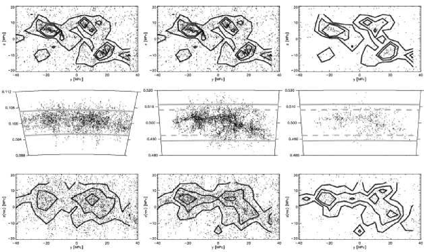
Figure 8: The distribution of ‘galaxies’ in the simulation. Panels in the left and central columns refer to a galaxy catalogue with limiting magnitude $M_{\rm I}=-20$, while panels in the right column refer to a catalogue with limiting magnitude $M_{\rm I}=-22$. Upper row: the galaxy distribution in cartesian coordinates, projected along the $x$-direction. Contour levels show regions with galaxy overdensities of 1, 2 and 3. Central row: the corresponding cone diagram. The galaxy distributions shown in the upper panels are displayed in the redshift space, by adding to the real positions the radial component of the galaxy velocities. The simulation box has been placed at a fictitious redshift: $z=0.1$ for the left panel, $z=0.5$ for the central and right panels. The solid lines mark the box size at the assumed redshifts, while the dashed lines correspond to the region in which haloes not belonging to the box, but having a peculiar velocity of $v\pm 1000$ km/s could fall: this is uded to indicate the region of incompleteness due to finiteness of the volume. Lower row: like the upper panels, but after recovering the cartesian coordinates from the redshift space. Again, contour levels show regions with galaxy overdensities of 1, 2 and 3.

In order to investigate these effects we create mock catalogues of ‘galaxies’ starting from the halo distribution extracted from the simulation and assuming a one-to-one relation between dark matter haloes and galaxies. Following an approach which is standard in semi-analytic modelling (see, e.g., De Lucia et al., 2004; Croton et al., 2006), we can associate to each object a magnitude by using a Tully-Fisher-like relation. In particular we adopt the best fit obtained by Giovanelli et al. (1997) from the analysis of 555 galaxies in 24 clusters:

$$M_{\rm I}-5\log h=-(21\pm 0.02)-(7.68\pm 0.13)(\log W-2.5)\ ,$$ (1)

where $M_{\rm I}$ is the absolute magnitude in the $I$-band and $W$ is the velocity width, which is simply related to the maximum circular velocity $V_{\rm max}$: $W=2V_{\rm max}$.

The distribution of the galaxies present in the HR region is shown in Fig. 8. In particular the upper panels refer to the real-space distribution, projected along the $x$-direction, for two different catalogues, with $M_{\rm I}<-22$ (corresponding to $V_{\rm max}>213$ km/s; left and central panels) and $M_{\rm I}<-20$ (corresponding to $V_{\rm max}>117$ km/s; right panel). We also show the isodensity contour levels corresponding to (projected) galaxy overdensities of 1, 2 and 3, computed by using pixels with size $5\times 5$ Mpc². It is easy to recognize the positions of the highest concentrations, where the four largest clusters are located, but it is also evident the presence of a connecting filamentary structure crossing the whole box, in particular when considering the deepest catalogue.

The previous plots do not include the systematic distortions due to the galaxy peculiar velocities $v$ which can wash out the filamentary pattern. To study their effect, we show also the cone diagrams (i.e. redshift vs. longitude; panels in the central row), produced by displacing the simulation box at a fictitious redshift and computing the galaxy positions in the redshift space, i.e. adding to the real position (converted in recession velocity through the Hubble law) the radial component of their peculiar velocities. Since the effect amplitude depends on the redshift at which we displace the box, we do two different choices: $z=0.1$ for the panel in the left column, $z=0.5$ for the panels in the central and right columns. To point out regions which can be affected by incompleteness problems related the finite simulation box, in the plots we also show the box size (solid lines) and the region in which possible haloes not belonging to this box, but having a peculiar velocity of $v\pm 1000$ km/s could fall (dashed lines). Elongated structures in the observer’ direction are well evident in the left panel showing the galaxy distribution at $z=0.1$: they are at the angular positions of the main clusters and correspond to the so-called ‘fingers-of-God’, also observed in real local surveys. However, due to the limited box size, the cone diagram is affected by the possible presence of a large number of interlopers. At higher redshift ($z=0.5$) fingers-of-God are much less prominent, while the wedge diagrams are dominated by an elongated structure which extends perpendicularly to the observer’ direction, similarly to the so-called ‘Great Wall’. The region which is sampled by our simulation without incompleteness problems is not completely filled by the galaxies and a filamentary pattern connecting the regions at highest density can be easily individuated.

Finally, we use the positions in the redshift space to recover the cartesian distribution of the galaxies. The results are shown in the lower panels of Fig. 8; again we overlay the isodensity contours corresponding to galaxy overdensities of 1, 2 and 3. As expected, the main structures appear significantly washed out, however the filament can be still clearly identified as an overdensity larger than 2. Moreover we find that the bright galaxies, although much less numerous, trace the filament much better.

Table 2: The density of haloes found in the bridges. Different columns present the results as a function of the minimum number of member particles $N_{\rm min}$, used in the halo definition; $M_{\rm min}$ is the corresponding approximate minimum mass (in units of $10^{11}M_{\odot}$). Lines 3 and 4 report the mean number density (in units of Mpc^-3) in the universe (adopting the mass function by Sheth & Tormen, 1999) and in the ZHR region, respectively. Lines 5 and 6 give the overdensity (computed with respect to the cosmic mean value) found in the bridges $A$-$C$ and $C$-$B$, respectively. Lines 7 and 8 give the overdensity (computed with respect to the ZHR box) found in the bridges $A$-$C$ and $C$-$B$, respectively.

$N_{\rm min}$	30	50	100	500	1000
$M_{\rm min}/10^{11}M_{\odot}$	0.28	0.46	0.93	4.65	9.30
mean density (Mpc-3)
in the universe	0.06	0.040	0.022	0.006	0.0032
in the ZHR region	0.11	0.072	0.043	0.019	0.0076
overdensity w.r.t. cosmic mean
bridge $A$-$C$	11.0	10.4	10.4	19.0	14.0
bridge $C$-$B$	9.7	9.5	9.8	14.9	11.2
overdensity w.r.t. ZHR region
bridge $A$-$C$	6.0	5.8	5.3	6.0	5.9
bridge $C$-$B$	5.3	5.3	5.0	4.7	4.7

5.2 X-ray emission

We consider now the X-ray emission of the gas in the filamentary structure. In particular we analyze here two-dimensional maps which have been created by following a standard procedure which exploits the SPH kernel to distribute on a pixel grid the desired quantities (X-ray surface brightness, SZ Compton-$y$ parameter, etc.). Details on the method can be found in Roncarelli et al. (2006) and Dolag et al. (2005).

The X-ray surface brightness (SB) was computed in the energy band [0.1-10] keV by adopting a cooling function $\Lambda(T)\propto\sqrt{T}$. Notice that this relation represents an approximation for temperatures smaller than 2 keV, where line cooling becomes important. The resulting maps are shown in the left column of Fig. 9. As expected, the emission is peaked in correspondence with the largest haloes: the positions of the four clusters $A$, $B$, $C$ and $D$ are easily recognizable in all three different projections. These objects appear as embedded in an extended low-SB region, but with no clear sign of a connecting structure between them. This is true even for the closest pair, located in the lower part of the first two panels. The presence of a large number of sources, which are not extended and having SB larger than $10^{-15}$ erg s^-1 cm^-2 arcmin^-2, is also evident in all maps: they correspond to isolated galaxies and/or small groups.

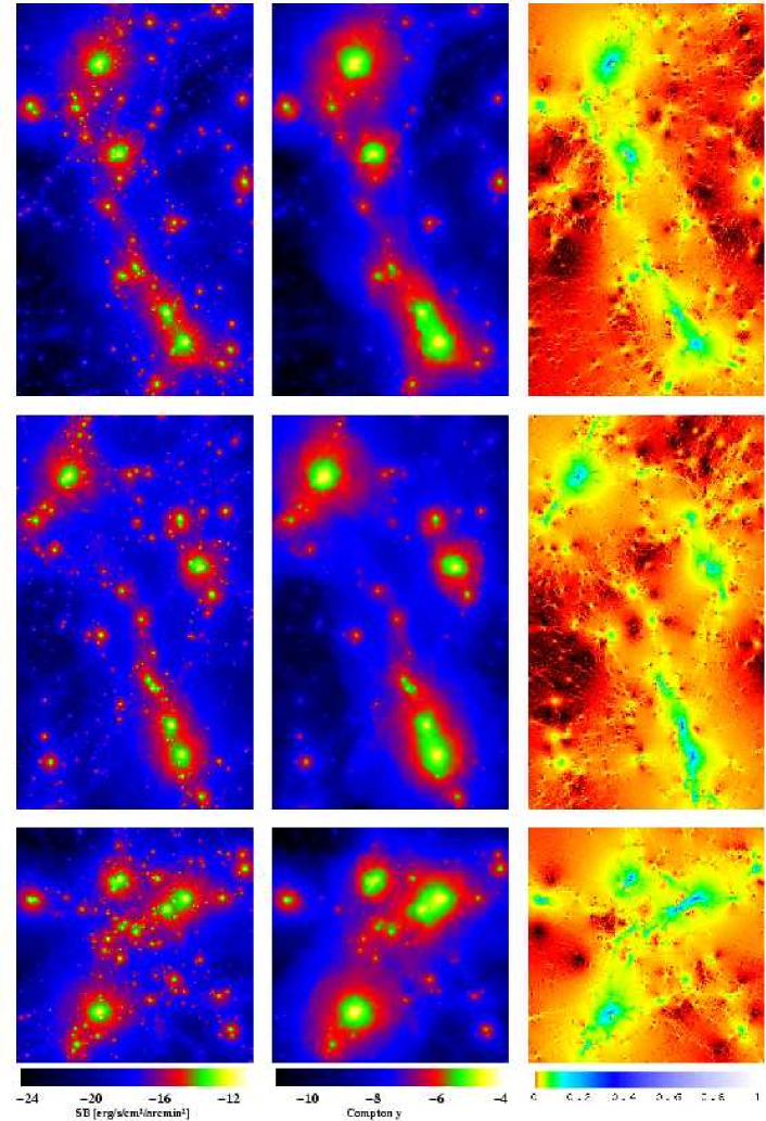
Figure 9: Projected maps of different observational quantities: the X-ray surface brightness (SB) produced by thermal bremsstrahlung (left column), the Compton-$y$ parameter quantifying the thermal Sunyaev-Zel’dovich effect (central column) and the amplitude of the reduced shear produced by weak gravitational lensing. The corresponding colour scales (which are logarithmic in the two first cases) are shown at the bottom. The displayed regions are the same as those shown in the rights panels of Fig. 1. Each row refers to a different cartesian projection: from top to bottom the projection is along the $z$, $x$ and $y$ axes.

Fig. 10 shows how the X-ray SB changes along the paths connecting the clusters, which were defined in the previous sections (see their positions in Fig. 1). The results refer to three different cartesian projections of the supercluster. The SB along the filaments is at least four orders of magnitude smaller than in the clusters. Indeed, while the SB corresponding to the largest haloes is of the order of $10^{-11}-10^{-13}$ erg s^-1 cm^-2 arcmin^-2, its value falls down to $10^{-16}-10^{-18}$ erg s^-1 cm^-2 arcmin^-2 in the lowest density regions of the bridges. Nevertheless, as we noticed earlier, many small substructures produce peaks of X-ray emission, reaching SB of the order of $10^{-14}$ erg s^-1 cm^-2 arcmin^-2. Therefore, the presence of the bridges seems to be more favourably revealed in the X-rays through compact sources, but certainly not through diffuse emission. This result is in qualitative agreement with the analysis made by Pierre et al. (2000), who found that filamentary structures cannot be clearly detected in the X-ray band because their signal would be confusion-dominated.

We would remark that our simulation includes non-radiative hydrodynamics only. It is well known that not considering cooling and feedback processes tends to change the X-ray emission properties of diffuse gas, decreasing the brightness in densest regions but enhancing the emissivity of the low-density material in the filaments (see, e.g., Bryan & Voit, 2001b). A parallel effect is the production of groups of galaxies which are overluminous with respect to real data (see, e.g., the discussion in Borgani et al., 2004). This makes the SB distribution more clumpy, and consequently can bias our estimates of the X-ray emission. This excess becomes evident by looking at the scaling relation between X-ray luminosity $L_{\rm X}$ and temperature $T$ (not shown): we find that our 27 main haloes scale (with some dispersion) like $L_{\rm X}\propto T^{2}$, as expected for non-radiative simulations, while the observed X-ray objects follow a steeper relation, in particular at the mass scales corresponding to galaxy groups (see, e.g., Osmond & Ponman, 2004).

Even if small, the emission from the filamentary regions could bias, via projection effects, the correct estimate of the cluster luminosities. In order to check this effect we compare the values obtained by considering the gas particles inside the virial radius only (see $L_{\rm X}$ reported in Table 1) to the values obtained by integrating the two-dimensional flux map, which also include the contribution of particles which appear inside the virial radius only in projection. In general we find that the increase of the luminosity is always smaller than 10 per cent. The only exception is the $y$-projection (last panel), where the two objects $B$ and $D$ are superimposed and appear as a unique (double) cluster: in this case the luminosity, which would be assigned to it, is very close to the sum of the (virial) luminosities of the two components.

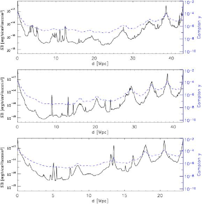
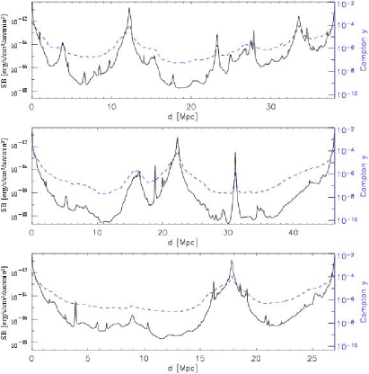
Figure 10: The behaviour of the X-ray SB (solid lines with units on the left) and SZ Compton-$y$ parameter (dashed lines with units on the right) along the filamentary paths. Left and right panels refer to the paths A-B-D and A-C-B, respectively. Each row shows a different cartesian projection, as in Fig. 9.

5.3 SZ effect

In the central column of Fig. 9 we show for the three different projections the resulting maps for the Compton-$y$ parameter: they are computed by applying a method similar to that adopted for the X-ray SB, i.e. using the SPH kernel. When compared to the corresponding X-ray maps, the signal appears as coming from more extended regions: this is the obvious consequence of the different dependence of the signal amplitude on the gas density. Unlike in the X-ray maps, the SZ maps reveal a weak evidence of the existence of two-dimensional structures connecting the most massive clusters. This is particularly evident in the last projection. This general result is confirmed by the trend of the Compton-$y$ parameter along the paths, shown in Fig. 10. The smallest substructures, from which a significant X-ray emission is coming, are not revealed by the SZ effect. On the contrary, the regions corresponding to the galaxy cluster signal are quite extended, with a smooth profile which is slowly declining outwards, with no evident signature of a transition at the virial radius. Along the bridges connecting the largest objects the Compton-$y$ parameter is very flat, with values of the order of $10^{-6}$. Outside the filaments, as can be read off the colour scale in Fig. 9, the Compton-$y$ parameter drops to values of the order of $10^{-9}-10^{-10}$. Notice that similar results have been obtained by Nath & Silk (2001), who estimated the heating of the ICM due to shocks arising from structure formation, with the aid of the Zel’dovich approximation.

In order to understand the impact of projection effects on the measurements of the SZ effect by the clusters embedded into the filamentary structure, we first evaluate $y$ towards the cluster centres considering only the gas particles which are contained in their virial regions. The mean of the values obtained considering three different cartesian projections is reported for each of the most massive clusters in Table 1. We find that, by varying the line of sight, the signal changes by up to 20 per cent for cluster $B$ and by up to 7 per cent for the other objects. Recalculating the Compton-$y$ parameter after including all gas particles within the ZHR box, we find that further fluctuations of the order of 10 per cent are possible. In practice changing the line of sight and including the effect produced by the surrounding filamentary structure can vary the measurement of the SZ effect for a cluster by up to 30 per cent.

Finally we notice that these estimates of the projection effects for both X-ray and SZ maps must be considered as lower limits, because in our analysis we are neglecting possible signals from unrelated foreground and background objects. This can be quite important for the SZ effect, where galaxy clusters are more extended structures than in the X-ray band, and consequently the probability of overlapping is much higher.

5.4 Weak gravitational lensing

Even if the observational detection of filaments via weak gravitational lensing is still largely uncertain (see the discussion in the introduction), it is certainly interesting to evaluate its potentiality by using numerical simulations. These are a useful tool for calibrating the methods and understand their reliability. First, we calculate the deflection angle field around the bridges. The method used here is described in more detail in a series of previous papers [see, e.g., Bartelmann et al. 1998; Meneghetti et al. 2000; Meneghetti et al. 2001; Meneghetti et al. 2003; Meneghetti et al. 2005]. We use as lens planes the mass maps obtained by projecting the three-dimensional mass distribution along the three lines-of-sight onto a regular grid of $1024\times 1024$ cells covering a region of 50 Mpc, adopting the same centre as in the previous analyses. The surface mass distributions have been smoothed by using the Triangular-Shaped-Cloud method (Hockney & Eastwood, 1988) for avoiding discontinuities which might introduce noise in the computation of the deflection fields. We propagate through another regular grid on the lens plane a bundle of $2048\times 2048$ light rays and compute for each of them the deflection angle $\vec{\hat{\alpha}}(\vec{\theta})$ as explained in Meneghetti et al. (2005). The reduced deflection angle is then defined as

$$\vec{\alpha}(\vec{\theta})\equiv\frac{D_{\rm ls}}{D_{\rm s}}\vec{\hat{\alpha}}(\vec{\theta})\ ,$$ (2)

where $D_{\rm ls}$ and $D_{\rm s}$ are the angular diameter distances between the lens and the source planes and between the observer and the source plane, respectively. For this analysis we shift the supercluster region to redshift $z_{\rm l}=0.3$. Moreover, we assume that all sources are at redshift $z_{\rm s}=2$, implying that the critical surface density,

$$\Sigma_{\rm crit}\equiv\frac{c^{2}}{4\pi G}\frac{D_{\rm s}}{D_{\rm l}D_{\rm ls}}=2.35\times 10^{15}\,\frac{M_{\odot}}{{\rm Mpc}^{2}}\ ,$$ (3)

is constant for all of them. In the former equation, $D_{\rm l}$ is the angular diameter distance between observer and lens. Although not realistic, our assumption substantially simplifies the following analysis and is acceptable because, for a lens at the redshift we consider here, the critical surface density changes little for typical sources having redshift $z>1$. For example, it varies by less than $25$ per cent when the source plane is moved from $z_{\rm s}=1$ to $z_{\rm s}=3$.

¿From the deflection angles $\vec{\alpha}(\vec{\theta})$, we can easily calculate both the convergence,

$$\kappa(\vec{\theta})=\frac{1}{2}\left(\frac{\partial\alpha_{1}}{\partial\theta_{1}}+\frac{\partial\alpha_{2}}{\partial\theta_{2}}\right)$$ (4)

and the two components of the shear,

$$\gamma_{1}(\vec{\theta}) = \frac{1}{2}\left(\frac{\partial\alpha_{1}}{\partial\theta_{1}}-\frac{\partial\alpha_{2}}{\partial\theta_{2}}\right)$$ (5)

$$\gamma_{2}(\vec{\theta}) = -\frac{\partial\alpha_{1}}{\partial\theta_{2}}=-\frac{\partial\alpha_{2}}{\partial\theta_{1}}\ .$$ (6)

We can then construct the complex shear as

$$\gamma=\gamma_{1}+i\gamma_{2}\ .$$ (7)

Finally the complex reduced shear is given by

$$g(\vec{\theta})=\frac{\gamma(\vec{\theta})}{1-\kappa(\vec{\theta})}\ .$$ (8)

This quantity is the expectation value of the observed ellipticity $\chi$ of the galaxies weakly distorted by the lensing effect. Measuring $\chi$ we thus obtain an estimate of the reduced shear, provided that we are in the weak lensing regime. The maps of the amplitude of the reduced shear obtained with this method and referring to the same regions investigated before are shown in the right panels of Fig. 9. Along the bridges, the reduced shear grows towards the clusters: in the cluster outskirts, it ranges between $\sim 0.05$ and $\sim 0.2$, while along the filaments it decreases to values of $\sim 0.01-0.02$.

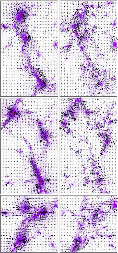
Figure 11: Maps for the reduced shear. Vectors (in arbitrary units) show the shear directions and are superimposed on the map of the absolute amplitude of the signal (already presented in the left column of Fig. 9). The displayed regions are the same presented in the right panels of Fig. 1. Each row refers to a different cartesian projection: from top to bottom the projection is along the $z$, $x$ and $y$ axes. The left column shows the total signal, while the right column the results obtained after removing the 27 most massive haloes identified in the simulation.

Since the shear from the galaxy clusters is so significantly dominant with respect to the shear caused by the filamentary structure, the distortion of the background galaxies is mainly tangential to the cluster concentrations rather than to the bridges of matter connecting them. This is evident in the left panels of Fig. 11, where the shear vectors are superimposed on the shear maps, previously shown. The same kind of distortion could in principle be produced by isolated clusters, i.e. not connected by any filament of matter. Together with the very low amplitude of the signal, this represents the more serious obstacle to the detection of the cosmic web via lensing effects.

In order to better quantify the filament signal, we repeat the same analysis but considering now what remains if the clusters in our field are removed, i.e. if the shear produced by their mass distributions is subtracted from the total shear. This is done by identifying in the simulation the particles within the virial radii of the individual clusters and using them for producing the deflection angle maps to be subtracted from the previous ones. Dealing with observations, we might try to provide a model for each individual cluster, calculate the shear it produces and remove it from the observed distortion of the background galaxies. In practice, as shown by Dietrich et al. (2005), it is very complex to find a way for separating the filaments from the clusters they connect, especially when considering close pairs of mass clumps. The results of this analysis are shown in the right panels of Fig.11. Here, we removed the shear produced by the particles belonging to the 27 most massive haloes found in the simulation, leaving the contributions from the filamentary structures and from the smallest clumps of matter only. The length of the vectors showing the shear orientation as well as the colour scale of the underlying shear maps are arbitrary. Along part of them the shear now turns to be tangential to the bridges, but still it is locally tangential to the remaining small mass concentrations.

On the basis of these simple considerations and considering the fact that the amplitude of the shear produced by the bridges is comparable to that provided by the large-scale structures along the line of sight to the distant galaxies, we can conclude that the detection of filamentary structures through their weak lensing signal is rather improbable. Dietrich et al. (2005) have recently proposed that techniques based on aperture multiple moments might be used for detecting filaments between close pairs of clusters. However, we believe that even this method seems to be difficult to apply for two main reasons: first, the noise produced by even the smallest clumps distributed or projected along the filament is large compared to the strength of the lensing signal from the filament itself; second, contaminations from the large-scale structure along the line of sight cannot be removed by using these techniques.

6 Conclusions

In this paper we discussed the physical and observational properties of the gas located inside the network of filaments constituting the cosmic web. For this aim, we used of the TreeSPH code GADGET-2 (Springel, 2005) to carry out a high-resolution hydrodynamical re-simulation of a supercluster-like structure. Suitable initial conditions were created on a specific region measuring about $50\times 50\times 70$ Mpc³, which was selected from a parent DM-only cosmological simulation because it contains several massive clusters connected by bridges and sheets of matter. The new simulation followed the evolution of the cosmic structure within the high-resolution region, reproducing the environmental properties of the larger cosmological box, from where it was taken. For the first time, it was possible to study at high resolution the formation of filaments between very massive clusters, taking non-radiative gas physics into account. The region selected contains 27 haloes with mass larger than $0.7\times 10^{14}M_{\odot}$, four of which with $M_{\rm vir}\raise-2.0pt\hbox{\hbox to0.0pt{\hbox{$\sim$}\hss}\raise 5.0pt\hbox{$>$}\ }10^{15}M_{\odot}$. The characteristics of the low-density filaments connecting the largest haloes were analyzed in more detail, with the aim of understanding how these filamentary structures may appear in view of their galaxy spatial distributions, X-ray emission and weak lensing signal. Indeed, these are properties which may be used to probe the existence of the cosmic web.

In particular we found:

• the cosmic web is formed by both two- and one-dimensional structures (sheets and filaments) which have a quite complex shape; the structure of the filaments along their length is characterized by changes in both the orientations of the axis of symmetry and in the thickness. The coherence length seems to be typically of the order of $\sim 5$ Mpc, but some segments of filaments can extend also to $\sim 25$ Mpc without significant changes in direction;

• by slicing a filament along its axis of symmetry, we find that these structures have diameters of the order of $\approx 3-5$ Mpc, within which the density contours appear round. Outside of this radius sheets of matter depart from the main structure. The thickness of the filament grows while approaching a cluster. The growth begins already at distances corresponding to $3-4$ times the virial radius of the cluster;

• the radial density profiles along filaments falls off less steeply than in galaxy clusters. The profile tends to become less steep, while the distance from the clusters increases. At large radii it gradually changes from being $\propto r^{-3}$ to being $\propto r^{-2}$;

• the typical values of the gas density in the bridges are between 10 and 100 times the cosmic mean value, increasing towards the clusters they bind and being smaller far from them;

• the thermal structure of the cosmic web is also quite complex, depending on the position of the accretion shocks, which, thanks to their movement outwards the galaxy clusters, tend to produce extended isothermal regions with $T_{MW}>5\times 10^{7}$ K extending to the filamentary structures;

• the velocity field also reflects the dynamics of structure formation, being orthogonal (aligned) to the filaments at large (small) distances from galaxy clusters.

In order to discuss the observable properties of the matter and the gas in the cosmic web, we produced maps of the halo distribution (which approximately reproduce the spatial distribution of galaxies), of the X-ray emission, of the thermal SZ effect and of the signal produced by the weak lensing effect. The main results of their analysis can be summarized as follows:

• inside the cosmic web the number density of haloes is about 10-14 times larger than the cosmic mean and 4-6 times larger than in the neighbourhood, almost irrespectively of the limiting mass considered. Galaxies seem to trace quite well the shape of the bridges between clusters, even when selection effects and redshift-space distortions are considered;

• in the X-ray maps the emission is peaked on galaxy clusters, which are surrounded by extended low-flux regions; along the filamentary structures, the surface brightness reaches at most $10^{-16}$ erg s^-1 cm^-2 arcmin^-2, except in the positions of small haloes (corresponding to isolated galaxies or groups), where the surface brightness can be even orders of magnitude larger. In the X-rays, the filaments thus appear as superpositions of relatively compact sources rather than as an extended region of diffuse emission;

• in the maps for the Compton-$y$ parameter, we found the evidence of a signal (with values of about $10^{-6}$) coming from the two-dimensional structures, connecting the main clusters. The signal comes from a more extended region compared to the X-ray emission, due to the weaker dependence of the Compton-$y$ parameter on the density;

• we estimated the typical bias on some observational properties of galaxy clusters produced by the projection of the surrounding filamentary network: we found an increase of less than 10 per cent for the X-ray luminosity and up to 30 per cent for the central Compton-$y$ parameter;

• we computed the reduced shear in the maps of the weak lensing signal, finding along the filaments very low values ($\sim 0.01-0.02$). The shear is rarely tangential to the filamentary structure. Rather, it is very often tangential to mass concentrations along the filamentary structure. Therefore, it seems very difficult to reveal the presence of filaments through weak lensing, even those connecting relatively close clusters.

In conclusion, our analysis confirms that filaments are very complex structures. They appear with very different features when looking at their galaxies, their gas or the distribution of their dark matter. In this paper we explored several observables which might be used to reveal the presence of the cosmic web. However the results here presented, in particular the low fluxes in the X-ray, the weak SZ effect and the very weak tangential shear signal, suggest that a conclusive detection of the filamentary structure will be a challenging problem also for future observations.

References

- Bardelli et al. (2000) Bardelli S., Zucca E., Zamorani G., Moscardini L., Scaramella R., 2000, MNRAS, 312, 540
- Bartelmann et al. (1998) Bartelmann M., Huss A., Colberg J. M., Jenkins A., Pearce F. R., 1998, A&A, 330, 1
- Bauer et al. (2004) Bauer F. E., Alexander D. M., Brandt W. N., Schneider D. P., Treister E., Hornschemeier A. E., Garmire G. P., 2004, AJ, 128, 2048
- Bharadwaj & Pandey (2004) Bharadwaj S., Pandey B., 2004, ApJ, 615, 1
- Bond et al. (1996) Bond J. R., Kofman L., Pogosyan D., 1996, Nat, 380, 603
- Borgani et al. (2004) Borgani S., et al., 2004, MNRAS, 348, 1078
- Brandt et al. (2001) Brandt W. N., et al., 2001, AJ, 122, 1
- Bregman et al. (2004) Bregman J. N., Dupke R. A., Miller E. D., 2004, ApJ, 614, 31
- Bryan & Norman (1998) Bryan G. L., Norman M. L., 1998, ApJ, 495, 80
- Bryan & Voit (2001a) Bryan G. L., Voit G. M., 2001a, ApJ, 556, 590
- Bryan & Voit (2001b) Bryan G. L., Voit G. M., 2001b, ApJ, 556, 590
- Cen & Ostriker (1999) Cen R., Ostriker J. P., 1999, ApJ, 514, 1
- Cheng et al. (2004) Cheng L.-M., Wu X.-P., Cooray A., 2004, A&A, 413, 65
- Colberg et al. (2005) Colberg J. M., Krughoff K. S., Connolly A. J., 2005, MNRAS, 359, 272
- Colberg et al. (1999) Colberg J. M., White S. D. M., Jenkins A., Pearce F. R., 1999, MNRAS, 308, 593
- Croft et al. (2001) Croft R. A. C., Di Matteo T., Davé R., Hernquist L., Katz N., Fardal M. A., Weinberg D. H., 2001, ApJ, 557, 67
- Croft et al. (2001) Croft R. A. C., Di Matteo T., Davé R., Hernquist L., Katz N., Fardal M. A., Weinberg D. H., 2001, ApJ, 557, 67
- Croton et al. (2006) Croton D. J., Springel V., White S. D. M., De Lucia G., Frenk C. S., Gao L., Jenkins A., Kauffmann G., Navarro J. F., Yoshida N., 2006, MNRAS, 365, 11
- da Silva et al. (2001) da Silva A. C., Kay S. T., Liddle A. R., Thomas P. A., Pearce F. R., Barbosa D., 2001, ApJ, 561, L15
- Davé et al. (2001) Davé R., et al., 2001, ApJ, 552, 473
- Dave et al. (1997) Dave R., Hellinger D., Primack J., Nolthenius R., Klypin A., 1997, MNRAS, 284, 607
- De Lucia et al. (2004) De Lucia G., Kauffmann G., White S. D. M., 2004, MNRAS, 349, 1101
- Dietrich et al. (2005) Dietrich J. P., Schneider P., Clowe D., Romano-Díaz E., Kerp J., 2005, A&A, 440, 453
- Dolag et al. (2005) Dolag K., Grasso D., Springel V., Tkachev I., 2005, Journal of Cosmology and Astro-Particle Physics, 1, 9
- Dolag et al. (2005) Dolag K., Hansen F. K., Roncarelli M., Moscardini L., 2005, MNRAS, 363, 29
- Doroshkevich et al. (1982) Doroshkevich A. G., Shandarin S. F., Zeldovich I. B., 1982, Comments on Astrophysics, 9, 265
- Ebeling et al. (2004) Ebeling H., Barrett E., Donovan D., 2004, ApJ, 609, L49
- Eke et al. (1996) Eke V. R., Cole S., Frenk C. S., 1996, MNRAS, 282, 263
- Finoguenov et al. (2003) Finoguenov A., Briel U. G., Henry J. P., 2003, A&A, 410, 777
- Gardini et al. (2004) Gardini A., Rasia E., Mazzotta P., Tormen G., De Grandi S., Moscardini L., 2004, MNRAS, 351, 505
- Gavazzi et al. (2004) Gavazzi R., Mellier Y., Fort B., Cuillandre J.-C., Dantel-Fort M., 2004, A&A, 422, 407
- Geller & Huchra (1989) Geller M. J., Huchra J. P., 1989, Science, 246, 897
- Giovanelli et al. (1997) Giovanelli R., Haynes M. P., da Costa L. N., Freudling W., Salzer J. J., Wegner G., 1997, ApJ, 477, L1
- Gray et al. (2002) Gray M. E., Taylor A. N., Meisenheimer K., Dye S., Wolf C., Thommes E., 2002, ApJ, 568, 141
- Hockney & Eastwood (1988) Hockney R. W., Eastwood J. W., 1988, Computer simulation using particles. Bristol: Hilger, 1988
- Jain et al. (2000) Jain B., Seljak U., White S., 2000, ApJ, 530, 547
- Jenkins et al. (2001) Jenkins A., Frenk C. S., White S. D. M., Colberg J. M., Cole S., Evrard A. E., Couchman H. M. P., Yoshida N., 2001, MNRAS, 321, 372
- Kaastra et al. (2003) Kaastra J. S., Lieu R., Tamura T., Paerels F. B. S., den Herder J. W., 2003, A&A, 397, 445
- Kaiser et al. (1998) Kaiser N., Wilson N., Luppino G., Romano-Diaz E., Kofman L., Gioia I., Metzger M., Dahle H., 1998, astro-ph/9809268
- Markevitch et al. (2003) Markevitch M., et al., 2003, ApJ, 583, 70
- Mathiesen & Evrard (2001) Mathiesen B. F., Evrard A. E., 2001, ApJ, 546, 100
- Mazzotta et al. (2004) Mazzotta P., Rasia E., Moscardini L., Tormen G., 2004, MNRAS, 354, 10
- Meneghetti et al. (2005) Meneghetti M., Bartelmann M., Dolag K., Moscardini L., Perrotta F., Baccigalupi C., Tormen G., 2005, A&A, 442, 413
- Meneghetti et al. (2003) Meneghetti M., Bartelmann M., Moscardini L., 2003, MNRAS, 346, 67
- Meneghetti et al. (2000) Meneghetti M., Bolzonella M., Bartelmann M., Moscardini L., Tormen G., 2000, MNRAS, 314, 338
- Meneghetti et al. (2001) Meneghetti M., Yoshida N., Bartelmann M., Moscardini L., Springel V., Tormen G., White S. D. M., 2001, MNRAS, 325, 435
- Nath & Silk (2001) Nath B. B., Silk J., 2001, MNRAS, 327, L5
- Navarro et al. (1997) Navarro J. F., Frenk C. S., White S. D. M., 1997, ApJ, 490, 493
- Osmond & Ponman (2004) Osmond J. P. F., Ponman T. J., 2004, MNRAS, 350, 1511
- Pandey & Bharadwaj (2005) Pandey B., Bharadwaj S., 2005, MNRAS, 357, 1068
- Peacock et al. (2001) Peacock J. A., et al., 2001, Nat, 410, 169
- Phillips et al. (2001) Phillips L. A., Ostriker J. P., Cen R., 2001, ApJ, 554, L9
- Pierre et al. (2000) Pierre M., Bryan G., Gastaud R., 2000, A&A, 356, 403
- Pimbblet (2005) Pimbblet K. A., 2005, MNRAS, 358, 256
- Pimbblet & Drinkwater (2004) Pimbblet K. A., Drinkwater M. J., 2004, MNRAS, 347, 137
- Pimbblet et al. (2004) Pimbblet K. A., Drinkwater M. J., Hawkrigg M. C., 2004, MNRAS, 354, L61
- Plionis et al. (2003) Plionis M., Benoist C., Maurogordato S., Ferrari C., Basilakos S., 2003, ApJ, 594, 144
- Porter & Raychaudhury (2005) Porter S. C., Raychaudhury S., 2005, MNRAS, 364, 1387
- Rasia et al. (2005) Rasia E., Mazzotta P., Borgani S., Moscardini L., Dolag K., Tormen G., Diaferio A., Murante G., 2005, ApJ, 618, L1
- Rasia et al. (2004) Rasia E., Tormen G., Moscardini L., 2004, MNRAS, 351, 237
- Roncarelli et al. (2006) Roncarelli M., Moscardini L., Tozzi P., Borgani S., Cheng L. M., Diaferio A., Dolag K., Murante G., 2006, MNRAS, 368, 74
- Rosati et al. (2002) Rosati P., Borgani S., Norman C., 2002, ARA&A, 40, 539
- Rosati et al. (2002) Rosati P., et al., 2002, ApJ, 566, 667
- Sathyaprakash et al. (1998) Sathyaprakash B. S., Sahni V., Shandarin S., 1998, ApJ, 508, 551
- Scharf et al. (2000) Scharf C., Donahue M., Voit G. M., Rosati P., Postman M., 2000, ApJ, 528, L73
- Sheth & Tormen (1999) Sheth R. K., Tormen G., 1999, MNRAS, 308, 119
- Springel (2005) Springel V., 2005, MNRAS, 364, 1105
- Springel & Hernquist (2002) Springel V., Hernquist L., 2002, MNRAS, 333, 649
- Springel et al. (2001) Springel V., White M., Hernquist L., 2001, ApJ, 549, 681
- Springel et al. (2001) Springel V., Yoshida N., White S. D. M., 2001, New Astronomy, 6, 79
- Tegmark et al. (2004) Tegmark M., et al., 2004, ApJ, 606, 702
- Thomas et al. (2001) Thomas P. A., Muanwong O., Pearce F. R., Couchman H. M. P., Edge A. C., Jenkins A., Onuora L., 2001, MNRAS, 324, 450
- Tormen et al. (1997) Tormen G., Bouchet F. R., White S. D. M., 1997, MNRAS, 286, 865
- Voit (2005) Voit G. M., 2005, Reviews of Modern Physics, 77, 207
- Voit & Bryan (2001) Voit G. M., Bryan G. L., 2001, ApJ, 551, L139
- White et al. (2002) White M., Hernquist L., Springel V., 2002, ApJ, 579, 16
- Worsley et al. (2005) Worsley M. A., et al., 2005, MNRAS, 357, 1281
- Xue & Wu (2003) Xue Y., Wu X., 2003, ApJ, 584, 34
- Yoshida et al. (2001) Yoshida N., et al., 2001, MNRAS, 325, 803
- Zappacosta et al. (2002) Zappacosta L., Mannucci F., Maiolino R., Gilli R., Ferrara A., Finoguenov A., Nagar N. M., Axon D. J., 2002, A&A, 394, 7