Mass Distributions of HST Galaxy Clusters from Gravitational Arcs

Abstract

Although $N$-body simulations of cosmic structure formation suggest that dark matter halos have density profiles shallower than isothermal at small radii and steeper at large radii, whether observed galaxy clusters follow this profile is still ambiguous. We use one such density profile, the asymmetric NFW profile, to model the mass distributions of 11 galaxy clusters with gravitational arcs observed by HST. We characterize the galaxy lenses in each cluster as NFW ellipsoids, each defined by an unknown scale convergence, scale radius, ellipticity, and position angle. For a given set of values of these parameters, we compute the arcs that would be produced by such a lens system. To define the goodness of fit to the observed arc system, we define a $\chi^{2}$ function encompassing the overlap between the observed and reproduced arcs as well as the agreement between the predicted arc sources and the observational constraints on the source system. We minimize this $\chi^{2}$ to find the values of the lens parameters that best reproduce the observed arc system in a given cluster. Here we report our best-fit lens parameters and corresponding mass estimates for each of the 11 lensing clusters. We find that cluster mass models based on lensing galaxies defined as NFW ellipsoids can accurately reproduce the observed arcs, and that the best-fit parameters to such a model fall within the reasonable ranges defined by simulations. These results assert NFW profiles as an effective model for the mass distributions of observed clusters.

1. Introduction

While numerical simulations of dark-matter halos in the CDM model of cosmic structure formation invariably predict density profiles which are steeper than isothermal outside and flatter inside a scale radius which is of order 20% the virial radius for cluster-sized halos (e.g. Navarro et al. 1997; Moore et al. 1998; Power et al. 2003; Navarro et al. 2004), it is yet unclear whether real galaxy clusters have such density profiles. Galaxy rotation curves (see Sofue & Rubin 2001 for a review) and strong-lensing constraints (e.g. Rusin & Ma 2001; Rusin et al. 2003; Treu & Koopmans 2004; Keeton 2001) have shown that galaxies need to have at least approximately isothermal density profiles which are however the result of baryonic physics such as gas cooling and star formation. In galaxy clusters, baryonic effects should be substantially weaker, and thus their density profiles outside the innermost cores should still reflect the typical CDM density profile found in numerical simulations.

Gravitational lensing has been used in its strong and weak variants for constraining the density profiles of clusters. Weak lensing measures the gravitational tidal field caused by mass distributions, and thus allows density profiles to be directly inferred. While there is agreement among most studies of weak cluster lensing that cluster density profiles are compatible with the shape proposed by Navarro et al. (1996, 1997) (hereafter NFW), they are typically similarly well fit by isothermal profiles (e.g. Clowe et al. 2000; Clowe & Schneider 2001; Sheldon et al. 2001; Athreya et al. 2002). The reason is that most of the weak-lensing signal comes from the cluster regions which surrounded the scale radius if the clusters had NFW density profiles, and there the NFW profile has an effective slope close to isothermal.

Strong lensing can happen in the cores of sufficiently dense and asymmetric clusters and gives rise to highly distorted, arc-like images. There are now well over 60 clusters known containing arcs with high length-to-width ratios. Mass models have been constructed for many of them, but mostly using axially-symmetric or elliptically distorted mass models with isothermal profiles. Several of these isothermal models turned out to be spectacularly successful (Kneib et al., 1993, 1996). Constructed based on few large arcs, they were detailed and accurate enough to predict counter-images of arclets found close to critical curves. Gavazzi et al. (2003) find that the core of MS 2137 seems to be closer to isothermal, while Kneib et al. (2003) give an example for a cluster which is better fit by NFW than isothermal mass components.

While models of strong lensing in clusters thus tend to favor density profiles steeper than expected from numerical simulations, Sand et al. (2004) followed Miralda-Escudé (1995) in combining the location of radial and tangential arcs with velocity-dispersion data on the central cluster galaxies and showed that cluster density profiles should be substantially less cuspy in their cores than even the NFW profile. This conclusion hinges on the assumption of axial cluster symmetry and can be shown to break down for even mildly elliptical mass models (Bartelmann & Meneghetti, 2004). However, the situation is obviously puzzling, and it seems appropriate to ask whether samples of arc clusters can be successfully modeled with appropriately asymmetric NFW mass components. This entails two questions; first, can cluster mass models based on mass components with NFW density profiles be found which reproduce the observed arcs; and second, are the best-fitting model parameters within reasonable ranges defined by simulations?

As our sample, we choose clusters which are known to have arcs and which have been imaged by the Hubble Space Telescope (HST). Our sample consists of 11 clusters: 3C 220, A 370, Cl 0016, Cl 0024, Cl 0054, Cl 0939, Cl 1409, Cl 2244, MS 0451, MS 1137, and MS 2137. We model each cluster with one or more elliptical NFW halos, each of which is completely defined by its scale convergence, scale radius, ellipticity, and position angle. In determining the values of these parameters that best reproduce the observed arcs, we constrain the mass distribution of the cluster. We find that all 11 clusters can be successfully modeled using elliptical NFW cluster mass profiles, and we tightly constrain the parameters defining each cluster’s mass distribution.

The rest of this paper is organized as follows: In § 2, we describe our method for estimating the parameters describing a cluster’s set of dark matter halos. In § 3, we define our error estimation for the derived parameters. In § 4, we test our method of estimating lens parameters on a simulated lensing cluster of known properties. In § 5, we outline our method of calculating the masses of our sample clusters. In § 6, we present results for each of the 11 clusters. Finally, in § 7, we discuss our main results and then summarize the implications of this work. Throughout this paper, we adopt a spatially flat cosmological model dominated by cold dark matter and a cosmological constant ($\Omega_{\mathrm{m0}}=0.3$, $\Omega_{\Lambda 0}=0.7$, $h=0.7$).

2. Lens Parameter Estimation

Approximately 85% of the matter in galaxy clusters is dark. If at all, gas cooling plays a substantial role only in their innermost cores, where the gas density may be high enough for cooling times to fall below the Hubble time. It is yet unclear what influence gas physics may have on strong cluster lensing. While adiabatic gas seems to have little effect, efficient cooling and star formation may steepen the density profile very near the cluster center and thus increase strong-lensing cross sections (Puchwein et al., 2005). In detail, any theoretical treatment of baryonic physics on strong cluster lensing depends on the numerical and artificial viscosity of the gas flow, the assumed star-formation efficiency, and the combination of a variety of feedback mechanisms. For simplicity, we shall here model each cluster in our sample as a combination of purely dark matter halos.

We model each dark matter halo with an asymmetric NFW profile. The spherical NFW density profile is

$$\rho(r)=\frac{\rho_{\mathrm{s}}}{(r/r_{\mathrm{s}})(1+r/r_{\mathrm{s}})^{2}}\;,$$ (1)

where $\rho_{\mathrm{s}}$ is a characteristic density and $r_{\mathrm{s}}$ is the scale radius, which describes where the density profile turns over from $\rho\propto r^{-1}$ to $\rho\propto r^{-3}$.

Following the common thin-lens approximation, the lens is approximated as a mass sheet perpendicular to the line-of-sight, and the scale convergence is defined as the ratio of surface mass densities, $\kappa_{\mathrm{s}}\equiv\rho_{\mathrm{s}}r_{\mathrm{s}}/\Sigma_{\mathrm{crit}}$, where $\Sigma_{\mathrm{crit}}$ is the critical surface mass density,

$$\Sigma_{\mathrm{crit}}\equiv\frac{c^{2}}{4\pi G}\,\frac{D_{\mathrm{s}}}{D_{\mathrm{l}}D_{\mathrm{ls}}}\;,$$ (2)

with the angular-diameter distances $D_{\mathrm{l,s,ls}}$ from the observer to the lens, to the source, and from the lens to the source, respectively.

Obviously, $\kappa_{\mathrm{s}}$ is valid for a single source redshift only. In clusters showing arcs at multiple redshifts, $\kappa_{\mathrm{s}}$ needs to be adapted in the following way. Assuming two source redshifts $z_{\mathrm{s}}^{(1)}$ and $z_{\mathrm{s}}^{(2)}>z_{\mathrm{s}}^{(1)}$ for simplicity, we refer $\kappa_{\mathrm{s}}$ to the lower source redshift $z_{\mathrm{s}}^{(1)}$. Fitting the lens model to the data, we adapt $\kappa_{\mathrm{s}}$ by the factor

$$f\equiv\frac{D_{\mathrm{ls}}^{(2)}}{D_{\mathrm{s}}^{(2)}}\,\frac{D_{\mathrm{s}}^{(1)}}{D_{\mathrm{ls}}^{(1)}}$$ (3)

for the more distant sources, where $D_{\mathrm{s}}^{(i)}\equiv D_{\mathrm{s}}(z_{\mathrm{s}}^{(i)})$ and $D_{\mathrm{ls}}^{(i)}\equiv D_{\mathrm{ls}}(z_{\mathrm{l}},z_{\mathrm{s}}^{(i)})$, with $z_{\mathrm{l}}$ as the lens redshift. Analogous factors are applied for sources at additional redshifts, if there are any.

To elliptically deform the mass distribution, we alter the potential to have ellipsoidal rather than axial symmetry. We accomplish this by defining the surface mass density $\Sigma$ to have a radial dependence described by the projected elliptical radius,

$$r_{\mathrm{e}}=\left[(r\cos\theta)^{2}(1-e)+(r\sin\theta)^{2}/(1-e)\right]^{1/2}\;,$$ (4)

rather than the circular radius $r$. We define the ellipticity $e=1-b/a$, where $a$ and $b$ are the major and minor axes respectively, and we define the position angle $\theta$ in degrees counterclockwise from the $+y$ axis.

For a given cosmology and halo redshift, an elliptical NFW halo depends on only four parameters: the scale convergence $\kappa_{\mathrm{s}}$, scale radius $r_{\mathrm{s}}$, ellipticity $e$, and position angle $\theta$. Numerical simulations predict that the halo concentration, i.e. the ratio between the virial radius $r_{200}$ and the scale radius $r_{\mathrm{s}}$, is determined by the halo mass, albeit with considerable scatter (Navarro et al., 1997; Bullock et al., 2001; Eke et al., 2001; Dolag et al., 2004). This implies that the two parameters $\rho_{\mathrm{s}}$ and $r_{\mathrm{s}}$ characterizing a spherically symmetric NFW halo are not independent. However, with the aim of testing numerical results using strong cluster lensing, we do not adopt any correlation between these two halo parameters.

We identify the arcs on the HST image of a cluster and define them by an array $(x_{i},y_{i})$ of $x$ and $y$ positions of the image points constituting each arc. These points are arranged on a grid with spacing $\sigma$ in $x$ and $y$. Generally, we take the spacing to be $\sigma=5$ HST pixels in order to limit the number of arc points. This array of grid positions forms the data set we use to define a cluster’s arcs.

We use SExtractor (Bertin & Arnouts, 1996) to define the position of each lens as its center of light on the HST image of the cluster. Then, for a given set of lens parameters ($\kappa_{\mathrm{s}}$, $r_{\mathrm{s}}$, $e$, $\theta$) for each lens, we use the lensing equations to map the arc data back to the source plane. This yields a set of points describing the source. We next use the lensing equations again to map the source points back to the lens plane by finding all images of all source points. The result is a set of points that defines the image of the source reproduced by the lens model. Our goal is to find the particular values of the lens parameters that yield predicted arcs that most closely match the arc data, the number of sources predicted by observations, and reasonably sized sources. Note that our approach does not require multiple arc-like images of a single source to be present and identified.

For this purpose we define a $\chi^{2}$ function of the lens parameters to quantify the goodness of fit of our model to the data, so that the minimum of $\chi^{2}$ produces the best fit. Our $\chi^{2}$ consists of three components.

First, we define how well each data point is fit by the image points by finding the image point that lies closest to a given data point. We introduce a $\chi^{2}$ component $\chi_{1}^{2}$ that depends on the distance between each data point and its closest image point. If we let the $N$ arc data points be ($x_{i},y_{i}$) and the closest predicted image point to a given data point be ($u_{\mathrm{cl},i},v_{\mathrm{cl},i}$), then this component of the $\chi^{2}$ is

$$\chi_{1}^{2}=\frac{1}{N}\,\sum^{N}_{i=1}\,\left[\frac{(x_{i}-u_{\mathrm{cl},i})^{2}}{\sigma^{2}}+\frac{(y_{i}-v_{\mathrm{cl},i})^{2}}{\sigma^{2}}\right]\;.$$ (5)

This $\chi_{1}^{2}$ thus implicitly assumes that the reproduced image points are distributed in a Gaussian fashion centered on the data points, with a standard deviation of $\sigma$.

Second, we define how well each image point is predicted by the data points by finding the data point that lies closest to a given image point. This is not redundant to the $\chi_{1}^{2}$ calculation above because even if every data point has a nearby image point, there may still be distant, errant image points which are close to no data points. We thus introduce another $\chi^{2}$ component $\chi_{2}^{2}$ that depends on the distance between each image point and its closest data point. If we let the $M$ predicted image points be ($u_{j},v_{j}$) and the closest data point to a given image point be ($x_{\mathrm{cl},j},y_{\mathrm{cl},j}$), then this component of the $\chi^{2}$ is

$$\chi_{2}^{2}=\frac{1}{M}\,\sum^{M}_{j=1}\,\left[\frac{(u_{j}-x_{\mathrm{cl},j})^{2}}{\sigma^{2}}+\frac{(v_{j}-y_{\mathrm{cl},j})^{2}}{\sigma^{2}}\right]\;,$$ (6)

assuming again a Gaussian distribution of data with respect to image points.

Third, we require that arcs which observations indicate are images of the same source indeed belong to a single source in our model. Some clusters host several families of arcs, each of which belongs to one unique source. We require that our model predicts both the number of sources suggested by observations of a cluster’s arcs as well as the correct correlation between individual arcs and sources, as suggested by observations. In addition, we require that the predicted source be small and compact, as lensed sources are commonly observed to be.

Define $N_{\mathrm{s}}$ as the number of sources suggested by observations to produce a given cluster’s set of arcs. We examine the $i$th source and its corresponding source points and image points predicted by our best-fit model to the cluster lens system. If we let the $P_{i}$ predicted source points be $(p_{i,j},q_{i,j})$, the mean $p_{i}$ position be $\bar{p}_{i}$, and the mean $q_{i}$ position be $\bar{q}_{i}$, then we define the contribution to $\chi^{2}$ from the source configuration as

$$\chi_{3}^{2}=\frac{1}{N_{\mathrm{s}}}\,\sum^{N_{\mathrm{s}}}_{i=1}\left(\frac{1}{P_{i}}\,\sum^{P_{i}}_{j=1}\,\left[\frac{(p_{i,j}-\bar{p}_{i})^{2}}{\sigma_{\mathrm{s}}^{2}}+\frac{(q_{i,j}-\bar{q}_{i})^{2}}{\sigma_{\mathrm{s}}^{2}}\right]\right)\;,$$ (7)

where the source points are assumed to have a Gaussian distribution with standard deviation $\sigma_{\mathrm{s}}$. The choice of $\sigma_{\mathrm{s}}$ is delicate as it controls the relative weight of the constraints in the lens plane, quantified by $\chi_{1,2}^{2}$, and in the source plane, quantified by $\chi_{3}^{2}$. Large values of $\sigma_{\mathrm{s}}$ may yield best fits with unreasonably large source configurations, while low values of $\sigma_{\mathrm{s}}$ may enforce very small sources at the expense of considerable deviations between image and data points. Thus, it may be necessary to try several fits with different choices of $\sigma_{\mathrm{s}}$ to obtain both good agreement between image and data points and compact sources.

We add these three components to yield our total $\chi^{2}$,

$$\chi^{2}=\chi_{1}^{2}+\chi_{2}^{2}+\chi_{3}^{2}\;.$$ (8)

By minimizing this quantity we maximize the overlap between data points and predicted image points, reproduce the number of sources indicated by observations, and require that the sources be reasonably small in size. Each combination of ($\kappa_{\mathrm{s}}$, $r_{\mathrm{s}}$, $e$, $\theta$) for each lens describes a different lens system that produces a different set of source and image points and hence a different $\chi^{2}$. We use a downhill-simplex minimization routine (“amoeba” from Press et al. 1992) to determine the combination of each lens’s ($\kappa_{\mathrm{s}}$, $r_{\mathrm{s}}$, $e$, $\theta$) that minimizes $\chi^{2}$. These best-fit values are the ones we use to define the cluster’s lens system.

3. Error Estimation

To estimate errors on the cluster dark matter halo parameters derived according to § 2, we employ $\chi^{2}$ statistics as outlined in Press et al. (1992). We must do so with caution. Formally, the $\chi^{2}$ function is the log-likelihood assuming Gaussian distributions of model points relative to data points. We cannot be sure that this accurately describes our situation, in which we need to quantify the deviation between given data and reproduced image points. Assuming Gaussian likelihood factors, the two contributions $\chi^{2}_{1,2}$ quantify the likelihoods of reproducing the data points with the image points, and of finding image points exclusively near data points. Taken as another contribution to $\chi^{2}$, $\chi_{3}^{2}$ quantifies the log-likelihood of the sources being well modeled as Gaussians with widths $\sigma_{\mathrm{s}}$. Strictly speaking, our $\chi^{2}$ is a figure-of-merit function as it quantifies the deviation of the model from the data in a well-defined sense. We shall, however, interpret it as a true $\chi^{2}$ function, i.e. assuming that all deviations can be described by appropriate Gaussians.

Recall that for a given lens system, the $\chi^{2}$ function reaches a minimum for the best-fit parameter values. Since its gradient vanishes at the minimum, the $\chi^{2}$ function can to lowest order of a Taylor expansion be described as parabolic in the neighborhood of the minimum. By varying each of the parameters around this minimum, we thus expect to follow a parabolic section along the parameter axes through the $\chi^{2}$ surface.

For a cluster with $N_{\mathrm{l}}$ lenses, each modeled with an ellipsoidal NFW density profile, we define a vector of best-fit parameters $\vec{a}_{\mathrm{bf}}=(\kappa_{\mathrm{s,bf,1}},r_{\mathrm{s,bf,1}},e_{\mathrm{bf,1}},\theta_{\mathrm{bf,1}},\ldots,\kappa_{\mathrm{s,bf,N_{\mathrm{l}}}},r_{\mathrm{s,bf,N_{\mathrm{l}}}},e_{\mathrm{bf,N_{\mathrm{l}}}},\theta_{\mathrm{bf,N_{\mathrm{l}}}})$. We then calculate the $16\,N_{\mathrm{l}}^{2}$ components of the curvature matrix $\alpha_{kl}$ by noting that

$$\alpha_{kl}=\frac{1}{2}\,\left.\frac{\partial^{2}\chi^{2}}{\partial a_{k}\partial a_{l}}\right|_{\vec{a}=\vec{a}_{\mathrm{bf}}}\;,$$ (9)

where $k$ and $l$ vary from 1 to $4N_{\mathrm{l}}$. The partial derivatives can be calculated from the parabolic fits along all parameter axes to the local $\chi^{2}$ function. The covariance matrix is the inverse of the curvature matrix, $C=\alpha^{-1}$, and the 1-$\sigma$ error in each parameter is $\delta a_{k}=\sqrt{C_{kk}}$. We generally find these errors to be of order a few percent. An interesting approach for estimating errors on strong-lensing model parameters based on Monte-Carlo Markov Chains was recently proposed by Brewer & Lewis (2005).

4. Comparison of Parameter Estimation Method with Simulations

To test our method of lens parameter estimation outlined in § 2, we use a numerically simulated galaxy cluster producing arcs.

The cluster was kindly made available by Klaus Dolag. It was obtained by re-simulating at higher resolution a patch of a pre-existing large scale numerical simulation of the $\Lambda$CDM model with parameters $\Omega_{\mathrm{m0}}=0.3$, $\Omega_{\Lambda 0}=0.7$, $H_{0}=70\,\mathrm{km\,s^{-1}\,Mpc^{-1}}$ and normalization $\sigma_{8}=0.9$. The “ZIC” technique used is described in detail in Tormen et al. (1997). The cluster has redshift $z=0.3$ and a virial mass of $M_{\mathrm{vir}}=2.29\times 10^{15}\,h^{-1}\,M_{\odot}$. The particle mass in the re-simulation is $m_{\mathrm{part}}=1.3\times 10^{9}\,h^{-1}\,M_{\odot}$. The gravitational softening is set to $5\,h^{-1}\,\mathrm{kpc}$.

We simulate lensing by this massive cluster using standard ray-tracing techniques. First, the particles contained in a cube of $3\,h^{-1}\,\mathrm{Mpc}$ comoving side length are selected. Then, to produce a two-dimensional density field, their masses are projected along the line of sight, interpolating their positions onto a regular grid of $256\times 256$ pixels using the Triangular Shaped Cloud method (Hockney & Eastwood, 1988). This surface density map, shown in Figure 1, is used as the lens plane in the following lensing simulation.

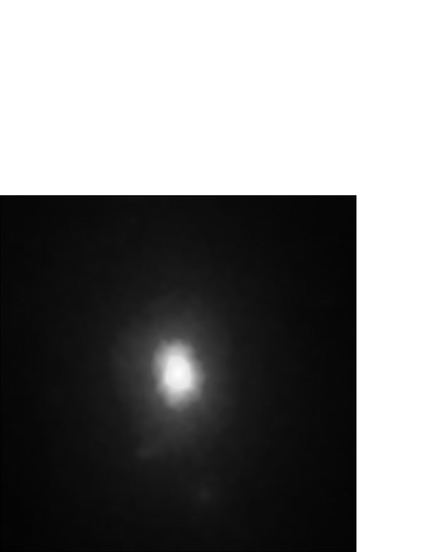
Figure 1.— A $\sim 370^{\prime\prime}\times 370^{\prime\prime}$ surface density map of the numerical cluster used to test our lens parameter estimation method.

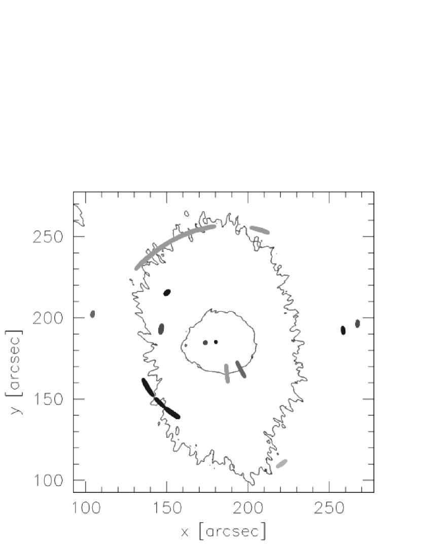
Figure 2.— The central region of Figure 1, illustrating the critical lines for the numerical cluster as well as examples of arcs produced by this cluster lens. We used such systems of arcs to test our method of lens parameter estimation.

A bundle of $2048\times 2048$ light rays is traced from the observer through the central quarter of the lens plane and their deflection due to the cluster mass distribution is calculated as described in several earlier papers (see e.g. Meneghetti et al. 2000, 2001, 2003b, 2003a). The arrival positions of the light rays on the source plane, which we place at redshift $z_{\mathrm{s}}=2$, are used to reconstruct the lensed images of several sources distributed around the caustic curves so as to produce strong lensing features. The sources are modeled as ellipses, with random orientation and axial ratios randomly drawn with equal probability from $[0.5,1]$. Their equivalent diameter (the diameter of the circle enclosing the same area as the source) is $r_{\mathrm{e}}=1^{\prime\prime}$. Several arc configurations have been used to test our method, and some of these are illustrated in Figure 2.

We conduct a blind test of our parameter estimation method by applying it to the simulated cluster and arcs without knowledge of any of the cluster’s physical properties but its position. We permit knowledge of the cluster’s position because when we model an HST cluster, we determine the positions of its galaxy lenses on the HST image with SExtractor.

We model the simulated cluster based on the cluster position and arc points, which is the same information we have when we model HST clusters. Applying the parameter estimation method described in § 2, we estimate the scale convergence, scale radius, ellipticity, and position angle of the simulated cluster. We then compare with the true values of these parameters in the simulated cluster mass distribution.

Table 1Best-fit parameters to lenses in the cluster sample.

Cluster	Lens	$\kappa_{\mathrm{s}}$	$r_{\mathrm{s}}\,(h^{-1}\,\mathrm{kpc})$	$e$	$\theta\,(^{\circ})$
Cl 2244$-$02		$0.178\pm 0.003$	$260\pm 20$	$0.113\pm 0.005$	$179\pm 1$
Abell 370	G1	$0.164\pm 0.007$	$254\pm 2$	$0.28\pm 0.01$	$78\pm 2$
	G2	$0.165\pm 0.004$	$212\pm 1$	$0.073\pm 0.004$	$167\pm 1$
3C 220.1		$0.178\pm 0.002$	$226\pm 4$	$0.265\pm 0.005$	$25\pm 1$
MS 2137$-$23		$0.67\pm 0.02$	$64\pm 2$	$0.11\pm 0.02$	$95\pm 3$
Cl 140933$+$5226		$0.099\pm 0.001$	$241\pm 2$	$0.033\pm 0.001$	$79\pm 2$
MS 0451.6$-$0305		$0.276\pm 0.006$	$262\pm 8$	$0.215\pm 0.004$	$156\pm 1$
MS 1137$+$66		$0.256\pm 0.002$	$279\pm 1$	$0.143\pm 0.005$	$58\pm 2$
Cl 0054$-$27	G1	$0.047\pm 0.001$	$340\pm 20$	$0.175\pm 0.003$	$92\pm 1$
	G2	$0.100\pm 0.001$	$259\pm 7$	$0.14\pm 0.01$	$18.6\pm 0.8$
Cl 0016$+$1609	DG 256	$0.102\pm 0.003$	$270\pm 10$	$0.123\pm 0.002$	$64.7\pm 0.4$
	DG 251	$0.087\pm 0.001$	$192\pm 4$	$0.121\pm 0.005$	$11.0\pm 0.5$
	DG 224	$0.219\pm 0.004$	$261\pm 7$	$0.1691\pm 0.0008$	$7.1\pm 0.4$
Cl 0939$+$4713	G1	$0.126\pm 0.005$	$136\pm 6$	$0.364\pm 0.008$	$2.65\pm 0.03$
	G2	$0.114\pm 0.002$	$190\pm 10$	$0.215\pm 0.008$	$73\pm 1$
	G3	$0.156\pm 0.005$	$170\pm 1$	$0.044\pm 0.003$	$87\pm 3$
Cl 0024$+$17	#362	$0.158\pm 0.003$	$198\pm 2$	$0.059\pm 0.002$	$6.6\pm 0.2$
	#374	$0.170\pm 0.002$	$250\pm 7$	$0.153\pm 0.006$	$135\pm 7$
	#380	$0.116\pm 0.003$	$285\pm 2$	$0.0020\pm 0.0001$	$58.1\pm 0.8$

Table 2Estimated cluster lens masses.

Cluster	Lens	$z_{\mathrm{arc}}$	$r_{\mathrm{s}}$	$M\,(\leq r_{\mathrm{s}})$	Reference
			$(h^{-1}\,\mathrm{kpc})$	$(h^{-1}\,M_{\odot})$
Cl 2244$-$02		2.237	260	$9.33\times 10^{13}$	1
Abell 370	G1	0.724/0.806/1.3	254	$1.31\times 10^{14}$	2
	G2	0.724/0.806/1.3	212	$9.21\times 10^{13}$	2
3C 220.1		1.49	226	$7.65\times 10^{13}$	3
MS 2137$-$23		1.501	64	$2.3\times 10^{13}$	4
Cl 140933$+$5226		2.811	241	$3.78\times 10^{13}$	5
MS 0451.6$-$0305		0.917/2.911	262	$2.38\times 10^{14}$	6
Cl 0939$+$4713	G1	3.98	136	$1.52\times 10^{13}$	7
	G2	3.98	190	$2.68\times 10^{13}$	7
	G3	3.98	170	$2.92\times 10^{13}$	7
Cl 0024$+$17	#362	1.675	198	$4.75\times 10^{13}$	8
	#374	1.675	250	$8.17\times 10^{13}$	8
	#380	1.675	285	$7.21\times 10^{13}$	8

References. — (1) Smail et al. (1997b); (2) Bézecourt et al. (1999); (3) Ota et al. (2000); (4) Gavazzi (2005); (5) Lubin et al. (2000); (6) Borys et al. (2004); (7) Trager et al. (1997); (8) Broadhurst et al. (2000).

In the simulation, the cluster is found to be well-described as an NFW ellipsoid with $\kappa_{\mathrm{s}}=0.54$, $r_{\mathrm{s}}=92.4^{\prime\prime}$, $e=0.18$, and $\theta=99^{\circ}$. With our arc modeling method, we found the cluster’s best-fit parameters to be $\kappa_{\mathrm{s}}=0.55$, $r_{\mathrm{s}}=88.9^{\prime\prime}$, $e=0.17$, and $\theta=96^{\circ}$, which are within 4% of the parameter values used to approximate the cluster. This is a convincing match, even more so because the true cluster parameters are the results of a fit and carry errors themselves. Hence, we proceed with confidence in our lens parameter estimation routine to model our sample of HST clusters.

5. Cluster Mass Estimates

If we know the lens parameters of a cluster and the source and lens redshifts, we can determine the mass of the lens within a given radius. We assume the lens is described by an NFW density profile, where the characteristic density is the density at the scale radius, given by $\rho_{\mathrm{s}}=\kappa_{\mathrm{s}}\Sigma_{\mathrm{crit}}/r_{\mathrm{s}}$. If we define $x\equiv r/r_{\mathrm{s}}$, then the mass contained within a (three-dimensional) radius $R$ is

$$M(\leq R) = 4\pi r_{\mathrm{s}}^{3}\rho_{\mathrm{s}}\,\int_{0}^{R}\frac{x^{2}\d{x}}{x(1+x)^{2}}$$ (10)

$$= 4\pi\Sigma_{\mathrm{crit}}\kappa_{\mathrm{s}}r_{\mathrm{s}}^{2}\,\left[\ln(1+y)-\frac{y}{1+y}\right]\;,$$

where $y\equiv R/r_{\mathrm{s}}$. The critical surface-mass density is given in equation (2).

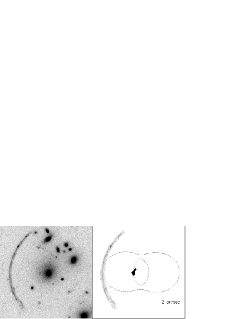
Figure 3.— A $20^{\prime\prime}\times 20^{\prime\prime}$ section of the F555W WFPC2 image of Cl 2244$-$02 (left) and the same section of the best fit (right). The plot on the right illustrates the reproduced giant arc (gray points), the predicted source (black points), and the lens’s critical curves. The gray image points are scaled such that darker grays denote brighter points in the image.

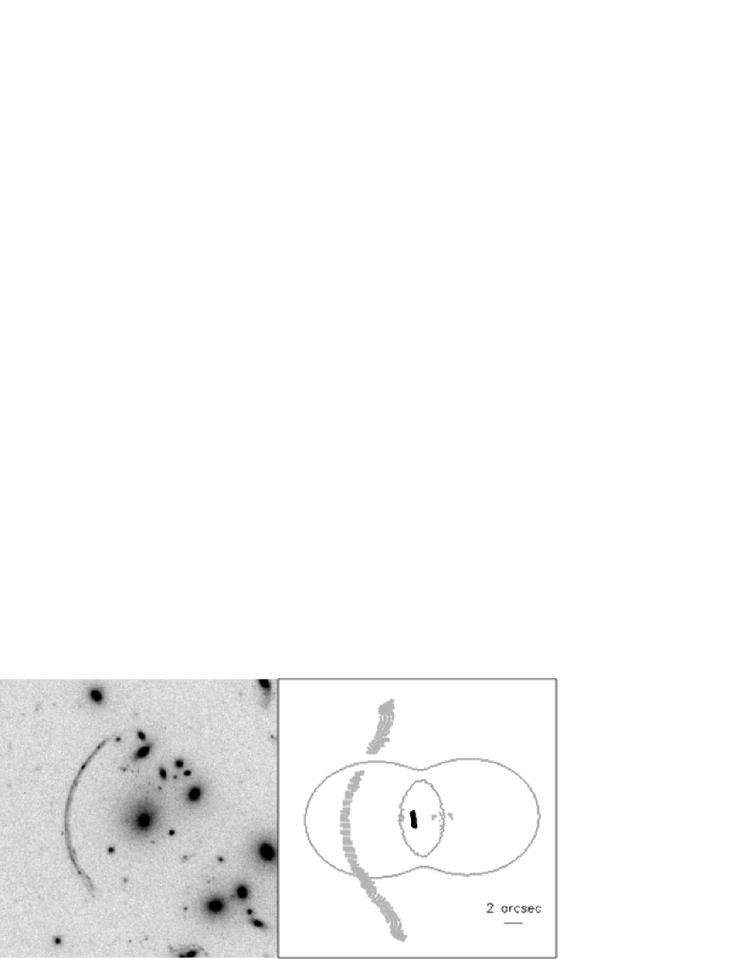
Figure 4.— As Figure 3, but enlarged to $30^{\prime\prime}\times 30^{\prime\prime}$ and using a model with lens parameters 3-$\sigma$ greater than the best-fit parameters (right).

For each lens in a cluster, we calculate the projected mass contained within the lens’s scale radius. We note that for the clusters in our sample without published arc redshifts (MS 1137, Cl 0054, and Cl 0016), we cannot estimate the lens masses.

6. Parameterizations and Mass Estimates of the Clusters

Here we present the best fit to each cluster based on the observed arcs, as described in § 2. We will discuss each cluster individually. For a summary of the best-fit parameters for all sampled clusters, see Table 1. Our mass results are summarized in Table 4, which includes the reference for each cluster’s arc redshifts.

• Cl 2244$-$02: The cluster Cl 2244$-$02 has a redshift $z=0.33$ and hosts a spectacular tangential arc (Smail et al., 1997b). Lynds & Petrosian (1989) discovered this giant luminous arc, which is located near the cluster center. The arc is a partial Einstein ring, and we take the lens to be the large galaxy seen in Figure 3 near where the Einstein ring is centered.

  Although the errors we calculated for the best-fit parameters are as small as half a percent, they are indeed realistic. In Figure 4 we illustrate what the predicted source and images would be for a lens defined by parameters 3-$\sigma$ greater than our best-fit values to Cl 2244$-$02. The predicted giant arc is much larger than that observed, and is broken into two sections. Also, two small images are produced near the source that are not seen in observations.

  Changing the lens parameters by only 3-$\sigma$ significantly alters the lensed images, which indicates that the lens parameters must be tightly constrained around our best-fit values. We use this example to justify the small errors we find for Cl 2244$-$02, and extend the argument also to the small errors we find for clusters that follow.

  

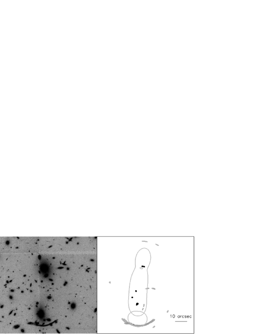
  Figure 5.— As Figure 3, showing an $80^{\prime\prime}\times 80^{\prime\prime}$ section of the F675W WFPC2 image of Abell 370.

  

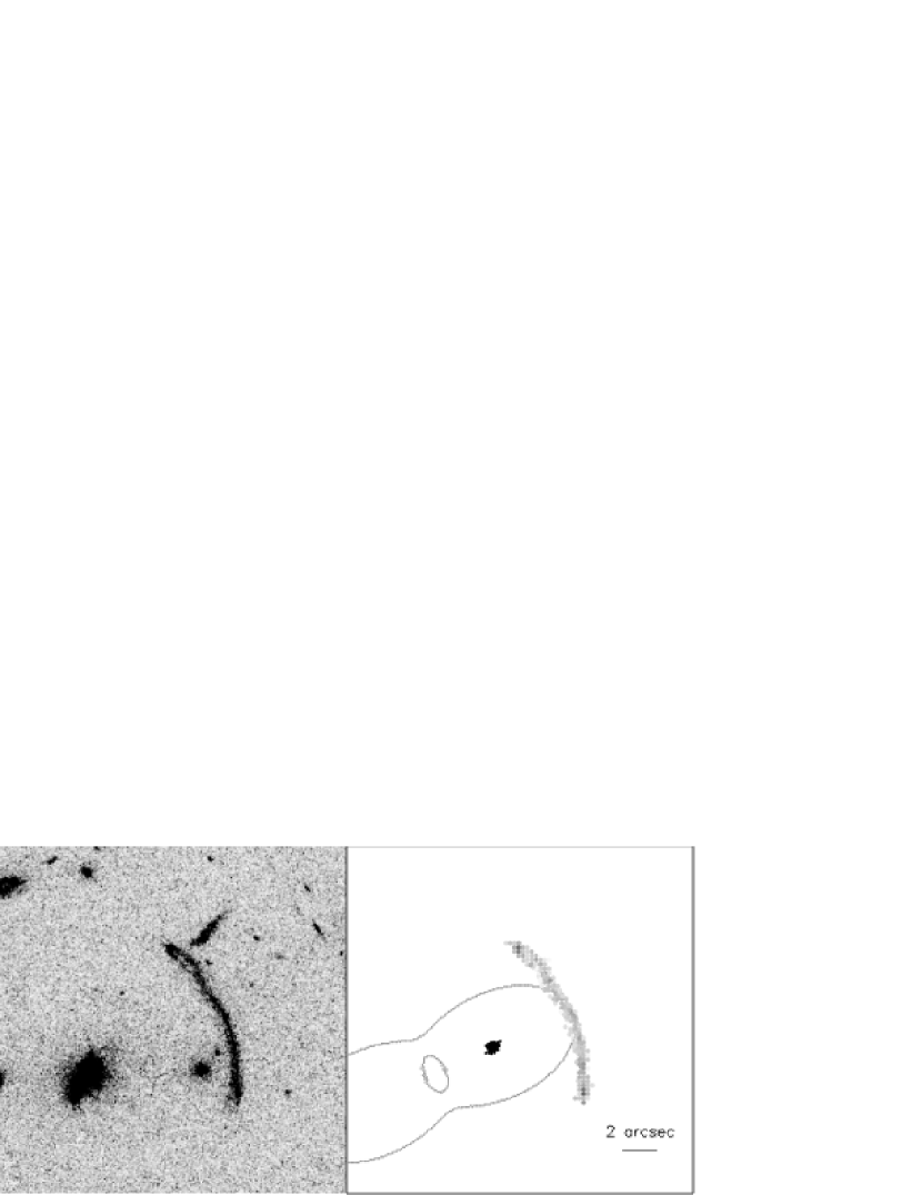
  Figure 6.— As Figure 3, showing a $20^{\prime\prime}\times 20^{\prime\prime}$ section of the F555W WFPC2 image of 3C 220.1.

• Abell 370: The rich cluster Abell 370 is at redshift $z=0.375$ (Abdelsalam et al., 1998) and has a bimodal mass distribution with two cD galaxies. These two galaxies mark the centers of two mass components in our model, and we identify the northern cD as G1 and the southern cD as G2.

  By the classification of Bézecourt et al. (1999), the giant arc is A0, the nearby radial and two tangential arcs are R, B2, and B3, and the upper tangential arcs are A1 and A2. These six arcs, as well as the cD galaxy lenses, are visible in Figure 5.

  We assume A1 and A2 to be at the same redshift as the dominant arc A0. They are likely to form a double image of the same source. Arcs B2 and B3 share the same redshift and are images of a separate source; R is an image of yet another source (Bézecourt et al., 1999). Accordingly, our best-fit model produces four independent sources for these six arcs.

  Our best fit also produces three additional images that we did not identify in our initial arc sample. They correspond to fuzzy patches on the HST image which may reflect actual images. The exact number of arcs in the cluster is unclear; Bézecourt et al. (1999) identify as many as 81 arclets. Further study would offer more insight into the complex nature of Abell 370.

  

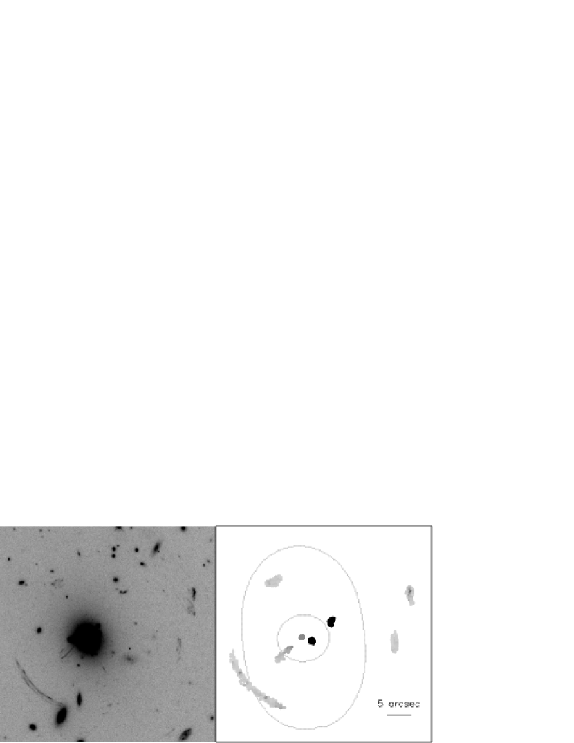
  Figure 7.— As Figure 3, showing a $45^{\prime\prime}\times 45^{\prime\prime}$ section of the F702W WFPC2 image of MS 2137$-$23.

  

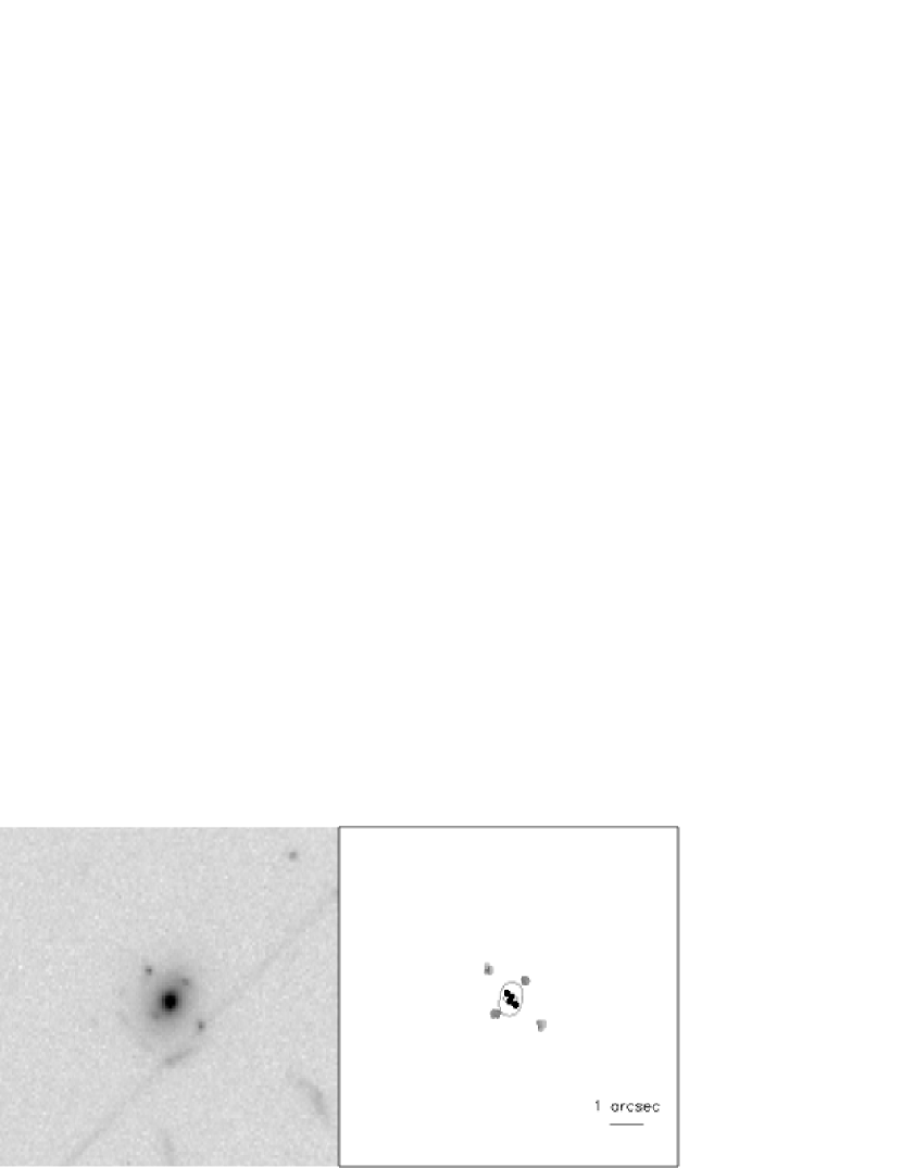
  Figure 8.— As Figure 3, showing a $10^{\prime\prime}\times 10^{\prime\prime}$ section of the F702W WFPC2 image of Cl 140933$+$5226.

• 3C 220.1: The cluster containing the radio galaxy 3C 220.1 is at redshift $z=0.62$ and hosts a giant arc (Ota et al., 2000). The lens responsible for producing this arc is 3C 220.1, which is identifiable as the largest source in the HST image on the left of Figure 6.

• MS 2137$-$23: MS 2137$-$23 is a rich cluster at redshift $z=0.313$ that contains a giant luminous arc and several arclets (Gavazzi, 2002). The cluster is dominated by a single cD galaxy, which we define as the lens. Adopting the classification system of Gavazzi (2002), the giant arc is A0, the radial arc near the cD galaxy is A1, the arc to the left of the cD galaxy in Figure 7 is A2, and the two arcs to the right of the cD galaxy are A4 and A5. The lens and the five arcs are visible in the HST image of MS 2137$-$23 shown in Figure 7.

  Gavazzi (2005) also fit an NFW model to MS 2137$-$23, and the ellipticity found in that paper is within the error bars of our best-fit ellipticity. However, our scale radius is $\sim 30\%$ smaller than, and our scale convergence is twice as large as, the corresponding values found in Gavazzi (2005). Despite these discrepancies, both our findings and those of Gavazzi (2005) agree that the concentration of the cD galaxy in MS 2137$-$23 is high.

  Our lens model predicts an additional arc, near the center of the cD galaxy, which was also discussed and possibly detected by Gavazzi et al. (2003). Gavazzi (2002) suggests that the arcs in MS 2137$-$23 can be categorized into two different systems, each with a unique source. The arcs A0, A2, and A4 are images of one source, and A1 and A5 are images of a separate source. We use these correlations to constrain the lens parameters, and Figure 7 illustrates the two unique sources predicted by our best-fit lens model.

  

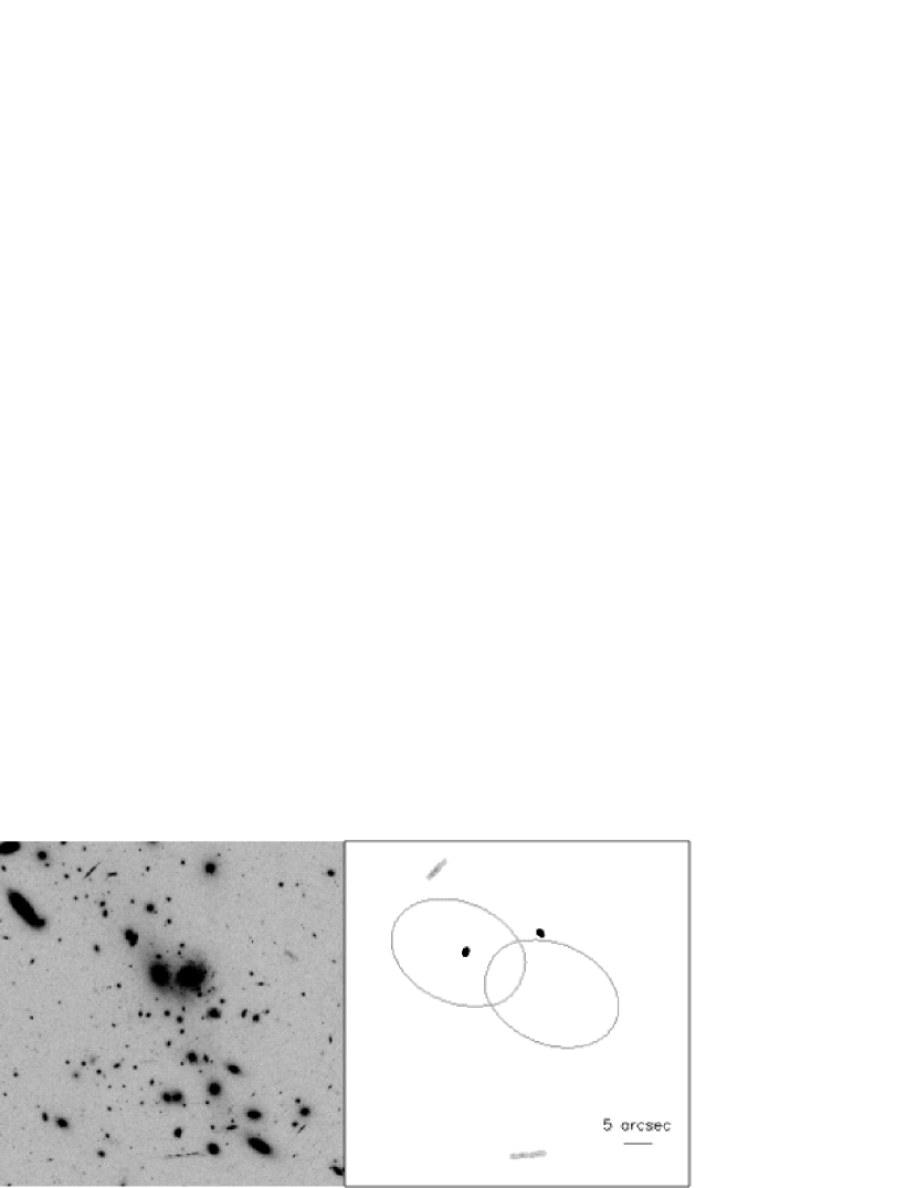
  Figure 9.— As Figure 3, showing a $60^{\prime\prime}\times 60^{\prime\prime}$ section of the F702W WFPC2 image of MS 0451.6$-$0305.

  

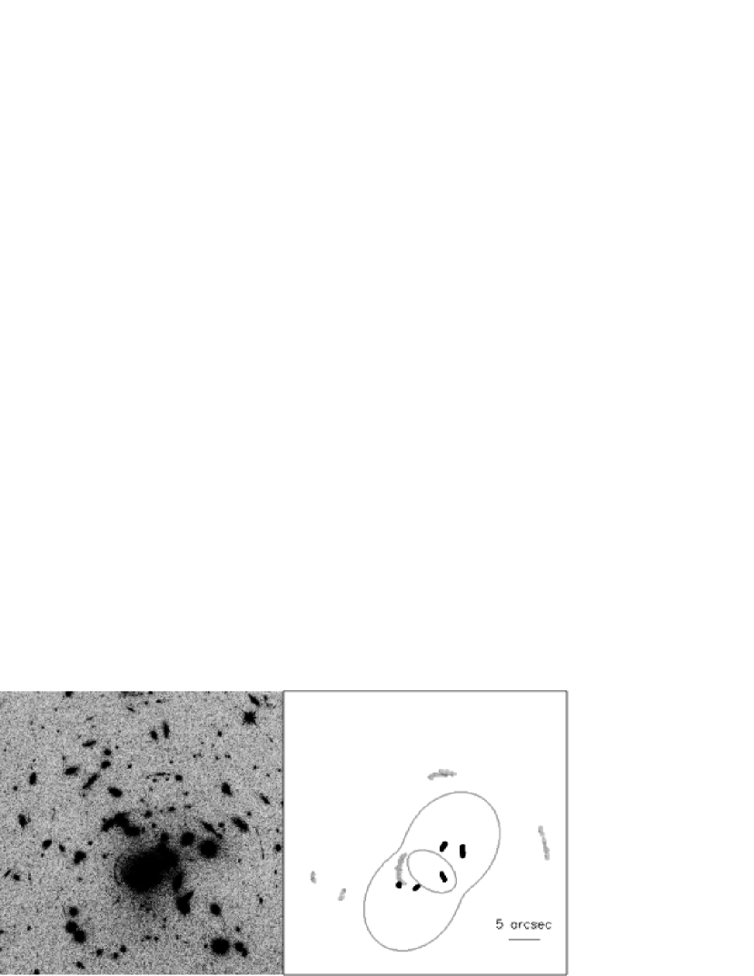
  Figure 10.— As Figure 3, showing a $45^{\prime\prime}\times 45^{\prime\prime}$ section of the F814W WFPC2 image of MS 1137$+$66.

• Cl 140933$+$5226: Fischer et al. (1998) discovered a quadruple lens in the $z=0.46$ cluster Cl 140933$+$5226, also known as 3C 295. The Einstein cross, as well as the lens galaxy at its center, is visible in Figure 8.

  As expected, the four images are due to a single source at the center of the Einstein cross.

• MS 0451.6$-$0305: The cluster MS 0451.6$-$0305 is located at $z=0.55$ and hosts two tangential arcs (Borys et al., 2004). The two arcs, as well as the cD galaxy lens, are apparent in the HST image in Figure 9. Following the classification of Borys et al. (2004), the lower arc in the figure is ARC1 and the upper arc is ARC2.

  Borys et al. (2004) note that the two arcs in MS 0451.6$-$0305 are at different redshifts and thus are not images of a single source. These two separate sources can be seen in our fit, shown in Figure 9.

  

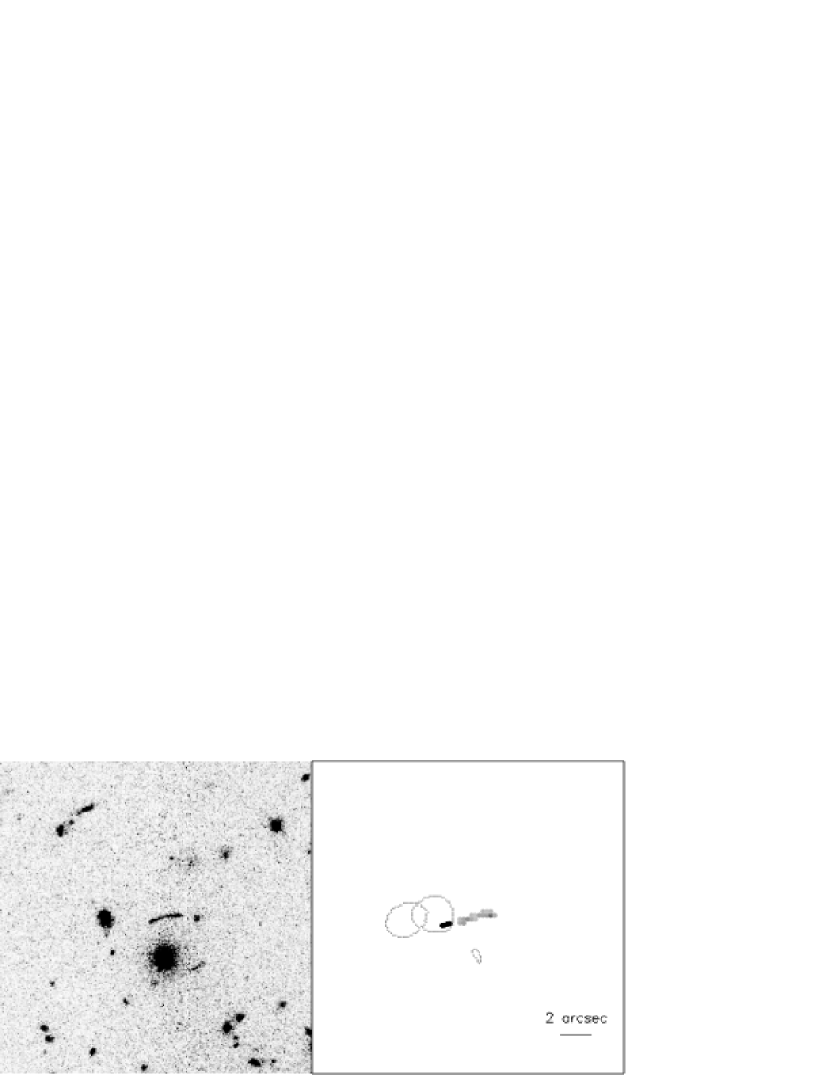
  Figure 11.— As Figure 3, showing a $20^{\prime\prime}\times 20^{\prime\prime}$ section of the F555W WFPC2 image of Cl 0054$-$27.

  

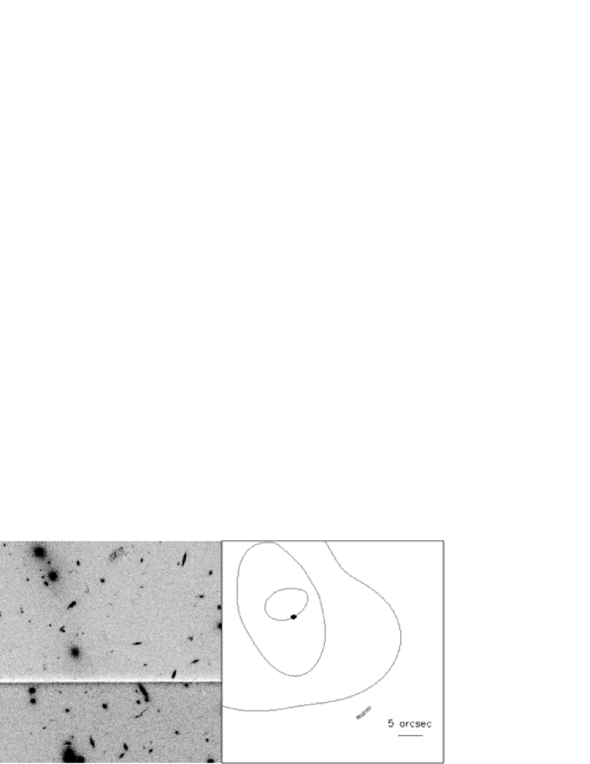
  Figure 12.— As Figure 3, showing a $45^{\prime\prime}\times 45^{\prime\prime}$ section of the F555W WFPC2 image of Cl 0016$+$1609.

• MS 1137$+$66: The lensing cluster MS 1137$+$66 at $z=0.783$ (Clowe et al., 1998) has the highest redshift of the clusters in our sample and hosts several faint arcs. We model five arcs, and because there are no published redshifts for the arcs, for simplicity we assume that they are all at the same redshift. The lens in our model is the cD galaxy at the center of the cluster.

  The lens defined by the parameters in Table 1 accurately reproduces the five observed arcs, as seen in Figure 10. Each arc has its own independent source.

  We cannot estimate the mass of the cD galaxy lens because there are no published redshifts for the arcs in MS 1137$+$66.

  

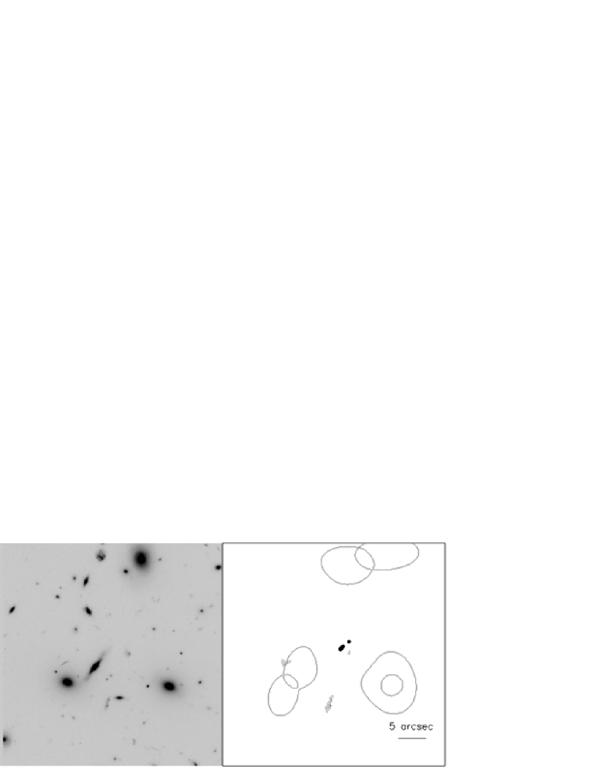
  Figure 13.— As Figure 3, showing a $40^{\prime\prime}\times 40^{\prime\prime}$ section of the F702W WFPC2 image of Cl 0939$+$4713.

  

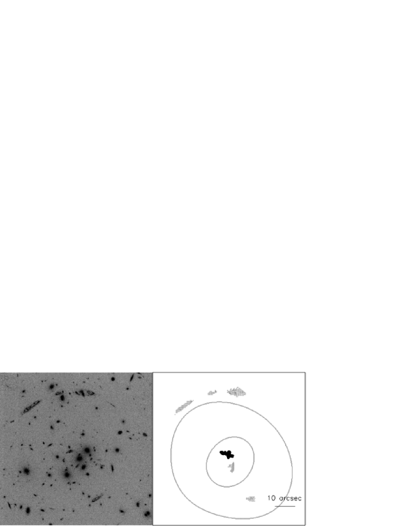
  Figure 14.— As Figure 3, showing a $75^{\prime\prime}\times 75^{\prime\prime}$ section of the F450W WFPC2 image of Cl 0024$+$17.

• Cl 0054$-$27: The cluster Cl 0054$-$27 is located at redshift $z=0.56$ and has one lensed arc (Smail et al., 1997a). To reproduce the arc, we take the two lenses in the cluster to be the central galaxy (which we call G1) and the upper left galaxy (which we call G2) in Figure 11.

  These two lenses combined reproduce the observed arc accurately. A mass estimate of the two lenses in Cl 0054$-$27 is impossible because there is no published redshift for the arc.

• Cl 0016$+$1609: The cluster Cl 0016$+$1609, at redshift $z=0.545$, has one thin lensed arc (Lavery, 1996). The three approximately collinear elliptical galaxies seen in Figure 12 define the center of the cluster and are the lenses we use to reproduce the observed arc. These three giant galaxies are, from top to bottom in Figure 12, DG 256, DG 251, and DG 224.

  The combination of these three lenses reproduces the single thin arc convincingly. Because there is no published redshift for the arc, we are unable to estimate the masses of the lenses in Cl 0016$+$1609.

• Cl 0939$+$4713: The cluster Cl 0939$+$4713 is at redshift $z=0.41$ and has three radial arcs near its center (Seitz et al., 1996). Three giant elliptical galaxies are visible in Figure 13, and these galaxies make up the cluster’s core. We take these galaxies to be the gravitational lenses, and call the upper one in Figure 13 G1, the leftmost one G2, and the rightmost one G3. The three arcs are also visible in Figure 13.

  Defined by their best-fit parameters given in Table 1, the three lenses are able to reproduce the three arcs observed in Cl 0939$+$4713. Trager et al. (1997) argue that two of the arcs in Cl 0939$+$4713 are likely images of the same source, whereas the third arc is probably an image of a separate galaxy. Consistent with this expectation, our model predicts two unique sources for the arc system.

• Cl 0024$+$17: The cluster Cl 0024$+$17 has redshift $z=0.395$ and hosts five images of a single background galaxy (Ota et al., 2004). The three central elliptical galaxies in the cluster, seen roughly collinear in Figure 14, act as the lenses for this system. From left to right in Figure 14, these galaxies are labeled #362, #374, and #380 in the Czoske et al. (2001) catalog.

  As lenses, these three central galaxies can accurately reproduce the five observed arcs in Cl 0024$+$17, as shown in Figure 14. Ota et al. (2004) note that all five arcs are images of a single background galaxy, and our results are consistent with that observation.

7. Conclusions

We have modeled 11 clusters hosting gravitational arcs and observed with HST as systems of dark matter halo lenses defined by elliptical NFW density profiles. Given its position on the HST image, each lens is completely defined by its scale convergence, scale radius, ellipticity, and position angle. We use a minimization routine to vary these parameters for each lens until the reproduced images match the observed arcs in the cluster, and each observationally confirmed family of arcs belongs to a unique source. We also require that the predicted sources are compact. With this routine, we find the best-fit scale convergence, scale radius, ellipticity, and position angle for each lens in each cluster.

Our main results can be summarized as follows:

1. Each cluster in our sample is successfully modeled as a system of mass components with asymmetric NFW density profiles. The model produces images that correspond to observed arcs in the cluster, and the system of arc sources suggested by observations is reproduced.

2. The best-fit parameters to each modeled cluster fall within the range of reasonable values set by simulations. Also, our estimates of the lens masses are reasonable for large galaxies.

3. The accuracy of our minimization technique for finding the best-fit parameters to a system of NFW ellipsoids is verified by our fit to a simulated cluster with arcs. The cluster was simulated as an NFW ellipsoid, and we successfully reproduced the simulated cluster’s parameters to within $4\%$.

Clusters containing arcs have been commonly and successfully modeled using mass components defined with spherical or ellipsoidal isothermal density profiles. We show, however, that galaxy clusters can also be convincingly modeled with NFW ellipsoids. The NFW profile is predicted for dark matter halos in numerical simulations of cosmological structure formation, and our result lends more credibility to NFW profiles as models of actual observed galaxy clusters.

References

- Abdelsalam et al. (1998) Abdelsalam, H. M., Saha, P., & Williams, L. L. R. 1998, MNRAS, 294, 734
- Athreya et al. (2002) Athreya, R., Mellier, Y., van Waerbeke, L., Fort, B., Pelló, R., & Dantel-Fort, M. 2002, A&A, 384, 743
- Bézecourt et al. (1999) Bézecourt, J., Kneib, J. P., Soucail, G., & Ebbels, T. M. D. 1999, A&A, 347, 21
- Bartelmann & Meneghetti (2004) Bartelmann, M., & Meneghetti, M. 2004, A&A, 418, 413
- Bertin & Arnouts (1996) Bertin, E., & Arnouts, S. 1996, A&AS, 117, 393
- Borys et al. (2004) Borys, C., Chapman, S., Donahue, M., Fahlman, G., Halpern, M., Kneib, J.-P., Newbury, P., Scott, D., & Smith, G. P. 2004, MNRAS, 352, 759
- Brewer & Lewis (2005) Brewer, B. J., & Lewis, G. F. 2005, ArXiv Astrophysics e-prints
- Broadhurst et al. (2000) Broadhurst, T., Huang, X., Frye, B., & Ellis, R. S. 2000, ApJ, 534, L15
- Bullock et al. (2001) Bullock, J., Kolatt, T., Sigad, Y., Somerville, R., Kravtsov, A., Klypin, A., Primack, J., & Dekel, A. 2001, MNRAS, 321, 559
- Clowe et al. (2000) Clowe, D., Luppino, G. A., Kaiser, N., & Gioia, I. M. 2000, ApJ, 539, 540
- Clowe et al. (1998) Clowe, D., Luppino, G. A., Kaiser, N., Henry, J. P., & Gioia, I. M. 1998, ApJ, 497, L61+
- Clowe & Schneider (2001) Clowe, D., & Schneider, P. 2001, A&A, 379, 384
- Czoske et al. (2001) Czoske, O., Kneib, J.-P., Soucail, G., Bridges, T. J., Mellier, Y., & Cuillandre, J.-C. 2001, A&A, 372, 391
- Dolag et al. (2004) Dolag, K., Bartelmann, M., Perrotta, F., Baccigalupi, C., et al. 2004, A&A, 416, 853
- Eke et al. (2001) Eke, V., Navarro, J., & Steinmetz, M. 2001, ApJ, 554, 114
- Fischer et al. (1998) Fischer, P., Schade, D., & Barrientos, L. F. 1998, ApJ, 503, L127+
- Gavazzi (2002) Gavazzi, R. 2002, New Astronomy Review, 46, 783
- Gavazzi (2005) Gavazzi, R. 2005, in IAU Symposium, 179–184
- Gavazzi et al. (2003) Gavazzi, R., Fort, B., Mellier, Y., Pelló, R., & Dantel-Fort, M. 2003, A&A, 403, 11
- Hockney & Eastwood (1988) Hockney, R., & Eastwood, J. 1988, Computer simulation using particles (Bristol: Hilger, 1988)
- Keeton (2001) Keeton, C. R. 2001, ApJ, 561, 46
- Kneib et al. (2003) Kneib, J., Hudelot, P., Ellis, R. S., Treu, T., Smith, G. P., Marshall, P., Czoske, O., Smail, I., & Natarajan, P. 2003, ApJ, 598, 804
- Kneib et al. (1993) Kneib, J., Mellier, Y., Fort, B., & Mathez, G. 1993, A&A, 273, 367
- Kneib et al. (1996) Kneib, J.-P., Ellis, R. S., Smail, I., Couch, W. J., & Sharples, R. M. 1996, ApJ, 471, 643
- Lavery (1996) Lavery, R. J. 1996, AJ, 112, 1812
- Lubin et al. (2000) Lubin, L. M., Fassnacht, C. D., Readhead, A. C. S., Blandford, R. D., & Kundić, T. 2000, AJ, 119, 451
- Lynds & Petrosian (1989) Lynds, R., & Petrosian, V. 1989, ApJ, 336, 1
- Meneghetti et al. (2003a) Meneghetti, M., Bartelmann, M., & Moscardini, L. 2003a, MNRAS, 346, 67
- Meneghetti et al. (2003b) —. 2003b, MNRAS, 340, 105
- Meneghetti et al. (2000) Meneghetti, M., Bolzonella, M., Bartelmann, M., Moscardini, L., & Tormen, G. 2000, MNRAS, 314, 338
- Meneghetti et al. (2001) Meneghetti, M., Yoshida, N., Bartelmann, M., Moscardini, L., Springel, V., Tormen, G., & White, S. 2001, MNRAS,, 325, 435
- Miralda-Escudé (1995) Miralda-Escudé, J. 1995, ApJ, 438, 514
- Moore et al. (1998) Moore, B., Governato, F., Quinn, T., Stadel, J., & Lake, G. 1998, ApJL, 499, L5
- Navarro et al. (1996) Navarro, J., Frenk, C., & White, S. 1996, ApJ, 462, 563
- Navarro et al. (1997) —. 1997, ApJ, 490, 493
- Navarro et al. (2004) Navarro, J. F., Hayashi, E., Power, C., Jenkins, A. R., Frenk, C. S., White, S. D. M., Springel, V., Stadel, J., & Quinn, T. R. 2004, MNRAS, 349, 1039
- Ota et al. (2000) Ota, N., Mitsuda, K., Hattori, M., & Mihara, T. 2000, ApJ, 530, 172
- Ota et al. (2004) Ota, N., Pointecouteau, E., Hattori, M., & Mitsuda, K. 2004, ApJ, 601, 120
- Power et al. (2003) Power, C., Navarro, J., Jenkins, A., Frenk, C., White, S., Springel, V., Stadel, J., & Quinn, T. 2003, MNRAS, 338, 14
- Press et al. (1992) Press, W., Teukolsky, S., Vetterling, W., & Flannery, B. 1992, Numerical Recipes in Fortran, 2nd edn. (Cambridge: Cambridge University Press)
- Puchwein et al. (2005) Puchwein, E., Bartelmann, M., Dolag, K., & Meneghetti, M. 2005, A&A, 442, 405
- Rusin et al. (2003) Rusin, D., Kochanek, C. S., & Keeton, C. R. 2003, ApJ, 595, 29
- Rusin & Ma (2001) Rusin, D., & Ma, C. 2001, ApJL, 549, L33
- Sand et al. (2004) Sand, D. J., Treu, T., Smith, G. P., & Ellis, R. S. 2004, ApJ, 604, 88
- Seitz et al. (1996) Seitz, C., Kneib, J.-P., Schneider, P., & Seitz, S. 1996, A&A, 314, 707
- Sheldon et al. (2001) Sheldon, E. S., Annis, J., Böhringer, H., Fischer, P., Frieman, J. A., Joffre, M., Johnston, D., McKay, T. A., Miller, C., Nichol, R. C., Stebbins, A., Voges, W., Anderson, S. F., Bahcall, N. A., Brinkmann, J., Brunner, R., Csabai, I., Fukugita, M., Hennessy, G. S., Ivezić, Ž., Lupton, R. H., Munn, J. A., Pier, J. R., & York, D. G. 2001, ApJ, 554, 881
- Smail et al. (1997a) Smail, I., Ellis, R. S., Dressler, A., Couch, W. J., Oemler, A. J., Sharples, R. M., & Butcher, H. 1997a, ApJ, 479, 70
- Smail et al. (1997b) Smail, I., Ivison, R. J., & Blain, A. W. 1997b, ApJL, 490, L5+
- Sofue & Rubin (2001) Sofue, Y., & Rubin, V. 2001, ARA&A, 39, 137
- Tormen et al. (1997) Tormen, G., Bouchet, F., & White, S. 1997, MNRAS, 286, 865
- Trager et al. (1997) Trager, S. C., Faber, S. M., Dressler, A., & Oemler, A. J. 1997, ApJ, 485, 92
- Treu & Koopmans (2004) Treu, T., & Koopmans, L. V. E. 2004, ApJ, 611, 739