Turbulent Mixing in the Outer Solar Nebula

Abstract

The effects of turbulence on the mixing of gases and dust in the outer Solar nebula are examined using 3-D MHD calculations in the shearing-box approximation with vertical stratification. The turbulence is driven by the magneto-rotational instability. The magnetic and hydrodynamic stresses in the turbulence correspond to an accretion time at the midplane about equal to the lifetimes of T Tauri disks, while accretion in the surface layers is thirty times faster. The mixing resulting from the turbulence is also fastest in the surface layers. The mixing rate is similar to the rate of radial exchange of orbital angular momentum, so that the Schmidt number is near unity. The vertical spreading of a trace species is well-matched by solutions of a damped wave equation when the flow is horizontally-averaged. The damped wave description can be used to inexpensively treat mixing in 1-D chemical models. However, even in calculations reaching a statistical steady state, the concentration at any given time varies substantially over horizontal planes, due to fluctuations in the rate and direction of the transport. In addition to mixing species that are formed under widely varying conditions, the turbulence intermittently forces the nebula away from local chemical equilibrium. The different transport rates in the surface layers and interior may affect estimates of the grain evolution and molecular abundances during the formation of the Solar system.

1 INTRODUCTION

The compositions of the gas giant planets and the comets reflect the conditions that were found in the outer Solar nebula. Jupiter, Saturn, Uranus and Neptune are enriched in volatiles relative to the Sun (Lunine et al., 2000; Young, 2003). The volatiles may have been accreted on the planets while trapped in ices (Lunine & Stevenson, 1985; Bar-Nun et al., 1988; Hersant et al., 2004), but the efficiency of this process depends on the poorly-known molecular compositions of the protoplanetary feeding zones, which depend in turn on the chemical reactions at work in different parts of the nebula and the effectiveness of transport by accretion and mixing. Some comets contain crystalline silicate grains (Wooden et al., 1999) and some have HCN molecules with deuterium to hydrogen ratios intermediate between the Sun and molecular clouds (Lunine et al., 2000). These results are puzzling because the midplane temperatures where the comets formed, near 30 AU, were too low for either the annealing of silicates or the destruction of primordial ices. The anomalous compositions of the comets could be due to gas and dust transported from the surface layers of the nebula or from nearer the Sun, where the temperatures were higher.

The molecular makeup of the Solar nebula was profoundly affected by chemical reactions in the gas phase and on grain surfaces, by ionizing radiation from the young Sun (Willacy & Langer, 2000) and by the mixing of materials formed at hot and cold locations (Morfill & Völk, 1984; Gail, 2001). Measurements of the millimeter molecular line fluxes in present-day protostellar disks are translated into abundances using detailed models in which the rates of transfer of material between different regions are a major uncertainty. Calculations without turbulent mixing indicate a layered structure in the outer nebula due to ultraviolet surface irradiation and interior freeze-out (Aikawa et al., 2002). Molecules such as CO and N₂ form from photodissociation products in warm surface layers, and freeze on grain surfaces near the midplane (Ceccarelli & Dominik, 2005). Including vertical turbulent mixing leads to significant changes in the chemical composition in models spanning radial distances 1–10 AU (Ilgner et al., 2004) as well as outside 100 AU (Willacy et al., 2006). The turbulence in these chemical models is assumed to act like a diffusion process. The importance of the mixing relative to the overall accretion flow toward the young star depends on the ratio between the material diffusion and angular momentum transfer coefficients (Stevenson, 1990), typically assumed to be unity.

The growth of solid bodies in protostellar disks depends fundamentally on the motions of the gas. Interstellar grains can grow larger than 30 $\mu$m in $10^{4}$ yr through collisions in turbulence of moderate strength (Suttner & Yorke, 2001). Small grains are removed so efficiently by coagulation that the overall infrared excess should fall below observed values long before the disk reaches an age of $10^{6}$ yr typical of T Tauri stars (Dullemond & Dominik, 2005). This problem may be resolved if the small particles are replenished by the break-up of aggregate grains in high-speed collisions. Many models of the particle size evolution include collisions resulting from a parametrized turbulence. The velocity fluctuations are often chosen to be an arbitrary fixed fraction of the sound speed and independent of height at each distance from the star. Better characterization of the turbulence is needed to further understand how the solid bodies are assembled.

A possible driver of turbulence in the Solar nebula is the magneto-rotational instability or MRI (Balbus & Hawley, 1991). The MRI occurs where weak magnetic fields are present and sufficiently coupled to the orbiting gas. Magnetic fields are detected in the molecular cloud cores that collapse to form protostars (Troland et al., 1996) and in the disks around T Tauri stars (Tamura et al., 1999). Remanent magnetization is found in meteoroids that solidified early in the history of the Solar system (Cisowski & Hood, 1991). The coupling between the disk gas and the fields depends on the conductivity. The outer Solar nebula was too cool for thermal ionization, and the conductivity is determined by balancing recombination on grain surfaces with the ionization due to cosmic rays (Wardle & Ng, 1999) or X-rays (Ilgner & Nelson, 2005). We are interested here in the region near the present orbit of Neptune, where the conductivity models indicate the MRI was active for reasonable grain parameters (Sano et al., 2000). The instability leads to turbulence in which accretion is driven by the transfer of orbital angular momentum outward along magnetic field lines (Hawley, Gammie, & Balbus, 1995). The mean accretion stress due to the magnetic forces is several times greater than that due to gas pressure gradients. The magnetic fields are anisotropic, with the azimuthal component strongest because of the differential rotation, the radial component next due to the radial stretching of field lines during the angular momentum transfer, and the vertical component weakest. The fields are buoyant, leading to the formation of a magnetized corona above and below the disk in calculations including the vertical stratification (Miller & Stone, 2000). The velocity dispersion in the corona is greater than in the disk interior.

Accretion and mixing act together to redistribute material through protostellar disks. Existing results on the relative importance of these two processes in MRI turbulence are as follows. The angular momentum transfer coefficient is an order of magnitude greater than the turbulent diffusion coefficient of a passive tracer species, in calculations with a net vertical magnetic field by Carballido et al. (2005) using the Zeus MHD code. On the other hand, the mixing of a dust fluid coupled to the gas by friction forces occurs at rates similar to the accretion in calculations with zero net magnetic flux by Johansen & Klahr (2005) using the Pencil code. Both studies involve unstratified shearing-box calculations. Our work resembles Carballido et al. (2005) in following a passive tracer with the Zeus code. We consider both zero and non-zero magnetic fluxes and include the effects of vertical stratification. The equations and method of solution are described in section 2, the domain and initial conditions in section 3. The results are divided into two sections. The spreading of an initial concentration enhancement in the turbulence is compared with solutions of a damped wave equation in section 4. The approximate steady state resulting from transport of material away from a fixed source and the chemical histories of individual Lagrangian fluid elements are discussed in section 5. A summary and conclusions are in section 6.

2 EQUATIONS AND METHOD OF SOLUTION

The domain is a small patch of the disk, centered at the midplane a distance $R$ from the axis of rotation. The effects of the radial gradient in orbital angular speed are treated using the local shearing box approximation (Hawley, Gammie, & Balbus, 1995) with vertical stratification included. Curvature along the direction of orbital motion is neglected, and the resulting Cartesian coordinate system co-rotates at the Keplerian orbital frequency $\Omega=\left(GM/R^{3}\right)^{1/2}$ for domain center with a stellar mass $M$. Coriolis and tidal forces in the rotating frame and the component of gravity perpendicular to the midplane are all included. The local coordinates $(x,y,z)$ correspond to distance from the domain center along the radial, orbital, and vertical directions, respectively. The azimuthal boundaries are periodic and the radial boundaries are shearing-periodic. Fluid passing through one radial boundary reappears on the other at an azimuth which varies in time according to the difference in orbital speed across the box. The difference is computed using a Keplerian profile linearized about domain center. The vertical boundaries are open and allow gas to flow out but not in.

The equations of isothermal ideal magnetohydrodynamics (MHD) are solved in the co-rotating frame. Conservation of mass and momentum and the evolution of magnetic fields are described by

$${{\partial\rho}\over{\partial t}}+{\bf\nabla\cdot}(\rho{\bf v})=0,$$ (1)

$${{\partial{\bf v}}\over{\partial t}}+{\bf v\cdot\nabla v}=-{{\bf\nabla}p\over\rho}+{1\over 4\pi\rho}({\bf\nabla\times B}){\bf\times B}-2{\bf\Omega\times v}+3\Omega^{2}{\bf\hat{x}}-\Omega^{2}{\bf\hat{z}},$$ (2)

and

$${\partial{\bf B}\over\partial t}={\bf\nabla\times}({\bf v\times B}),$$ (3)

together with the isothermal equation of state $p=c_{s}^{2}\rho$, which depends on the isothermal sound speed, $c_{s}$. The density, velocity, gas pressure and magnetic field are $\rho$, ${\bf v}$, $p$ and ${\bf B}$, respectively. The equations are integrated using the standard Zeus code (Stone & Norman, 1992a, b; Hawley & Stone, 1995). The flow of a trace contaminant is followed by solving an additional continuity equation

$${{\partial C}\over{\partial t}}+{\bf\nabla\cdot}(C{\bf v})=0$$ (4)

for the volume mass density, $C$.

We also wish to track the paths of individual fluid elements through the flow. Advanced trajectory integration methods offer few benefits here because MRI-driven turbulence is chaotic and the streamlines diverge exponentially with an $e$-folding time similar to the orbital period (Winters et al., 2003). An appropriate choice is an integration method that is slightly more accurate than the hydrodynamic part of the calculations. We use a classical fourth-order Runge-Kutta particle orbit integrator. Gas quantities are interpolated to the particle positions using the same second-order accuracy as in the hydrodynamics. Tests show the method has the expected order of convergence. In one example, a washing-machine problem, a circulating velocity field oscillates in time. The error in the particle position has the $(\Delta t)^{4}$ dependence of the fourth-order method and is dominated by roundoff error when the number of timesteps per oscillation is large.

3 DOMAIN AND INITIAL CONDITIONS

The surface density and temperature for the calculations are chosen based on observations of disks around T Tauri stars. The domain is centered 30 AU from an object of one Solar mass so that the orbital period $2\pi/\Omega=164$ years. The surface density $\Sigma=25$ g cm^-2 is consistent with fits to the spectral energy distributions of young stars (D’Alessio et al., 2001). The equilibrium temperature of a blackbody 30 AU from the Sun is 50 K, but detailed radiative transfer calculations show the midplane of the Solar nebula was colder than a blackbody in direct sunlight, due to the obscuration by the inner disk. For a T Tauri star of 0.5 Solar mass and 0.9 Solar luminosity, the midplane temperature at 30 AU is estimated to be about 25 K (D’Alessio et al., 2001). Temperatures above and below the midplane are greater because the material is externally-heated by thermal emission from grains in surface layers exposed to the stellar irradiation (Chiang & Goldreich, 1997). For our calculations spanning the midplane we use an isothermal equation of state with temperature $T=25$ K throughout. The optical depth of the disk to its own thermal radiation is about 0.05, so that internal temperature fluctuations are quickly erased by radiation losses.

The initial state is in radial and vertical hydrostatic equilibrium. The density varies with height as $\rho=\rho_{0}\exp({-z^{2}/2H^{2}})$ having scale height $H=c_{s}/\Omega=1.64$ AU. The uniform sound speed $c_{s}=0.298$ km s^-1 is appropriate for a mean molecular weight $\mu=2.34$, while the midplane density $\rho_{0}=4.05\times 10^{-13}$ g cm^-3 is chosen to give the desired surface mass density. The resulting structure is locally gravitationally stable, as the Toomre parameter $Q=\Omega c_{s}/(\pi G\Sigma)=7$. Small dust particles are well-coupled to the gas throughout the domain by the Epstein drag force. Compact spherical ice grains less than 100 $\mu$m in radius have any motions with respect to the gas damped within 0.1 orbits even at the lowest gas densities.

The coupling between gas and magnetic fields in the outer Solar nebula depends on the balance between recombination on grain surfaces and ionization by cosmic rays and X-rays. The conductivity varies with the total grain surface area per unit gas mass (Wardle & Ng, 1999). For an interstellar particle size distribution, the surface area lies mostly on the smallest grains of about 0.005 $\mu$m (Draine & Lee, 1984). Under the conditions at the midplane in our calculations, the free charge resides largely on the grains, the ionization fraction is very low, and the magneto-rotational instability is absent (Sano et al., 2000). However if the smallest grains are agglomerated into larger bodies and the remaining surface area is dominated by 0.1-$\mu$m grains, the largest contributions to the conductivity are from electrons and ions (Wardle & Ng, 1999). The conductivity is ample for MRI (Sano et al., 2000), but ambipolar diffusion may be present. Ambipolar diffusion can lead to weaker turbulence (Hawley & Stone, 1998). If the grain surface area is reduced to negligible levels and the magnetic pressure is much less than the gas pressure, the Hall term is the largest non-ideal effect (Sano & Stone, 2002a; Salmeron & Wardle, 2005). The magnetic field is tied to the gas and the instability leads to turbulence with properties similar to those in ideal MHD (Sano & Stone, 2002b). Given the rapid removal of small grains by coagulation in the existing models (Dullemond & Dominik, 2005) and the observational evidence for grains in disks larger than in the interstellar medium (Cotera et al., 2001; D’Alessio et al., 2001; McCabe et al., 2003; Shuping et al., 2003), we consider the case where gas and fields are well-coupled.

The initial $y$-velocities in our calculations are chosen for radial force balance between gravity and rotation. The $x$- and $z$-velocities in each grid zone are initially set to random values with maximum magnitudes 1% of the sound speed. The domain size in the radial, azimuthal and vertical directions is $L_{x}\times L_{y}\times L_{z}=3\times 12\times 12$ AU and the grid extends $3.7H$ either side of the midplane. The standard resolution is $32\times 64\times 128$ grid zones, corresponding to a zone aspect ratio $1:2:1$. An additional calculation is made with the spatial resolution doubled giving twice as many zones along each direction.

The magnetic field has zero net flux. The vertical component is initially proportional to $\sin\left(2\pi x/L_{x}\right)$ and the azimuthal component to $\cos\left(2\pi x/L_{x}\right)$, so that the field lines are straight, the magnetic pressure is uniform and there are no magnetic forces. The initial field strength $4.9\times 10^{-3}$ Gauss corresponds to a magnetic pressure 379 times smaller than the midplane gas pressure $\rho_{0}c_{s}^{2}$. The wavelength $2\pi v_{A}/\Omega$ of the magneto-rotational instability at the midplane is eight times the vertical grid spacing or $0.45H$. During the calculations, large Alfvén speeds $v_{A}$ and small timesteps are prevented by imposing a density floor $10^{-18}$ g cm^-3 that lies in the range expected for material falling in from a surrounding protostellar envelope. A check on the effects of the density floor is described in section 4.2. The field on the vertical boundaries is evolved by applying the condition $\partial{\bf\cal E}/\partial z=0$ to the electromotive force ${\bf\cal E}\equiv{\bf v\times B}$.

At the start of each calculation, the magneto-rotational instability grows to non-linear amplitudes over about two orbits. The flow then becomes turbulent and after four orbits the total kinetic energy varies little with time. At ten orbits, the magnetic field is thoroughly tangled and the flow has reached a time-averaged steady state. A contaminant is then added and its motions tracked.

4 SPREADING OF AN INITIAL CONCENTRATION ENHANCEMENT

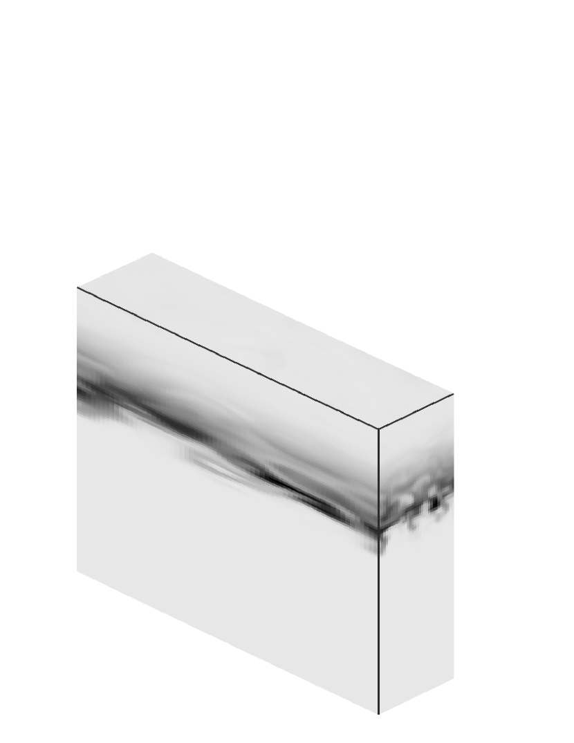
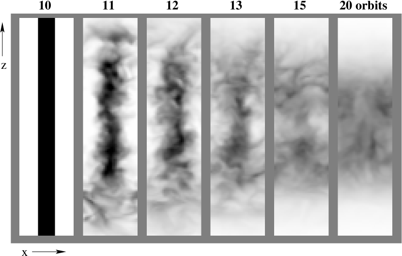
In the fiducial calculation, the contaminant is initially placed in a thin horizontal layer, centered 3 AU above the midplane and 0.375 AU thick. The density of the contaminant is set to $C_{0}$ in the layer and zero elsewhere. The contaminant spreads irregularly due to the turbulent motions, as shown in figure 1 by a snapshot at 15 orbits.

Figure 1: Spreading of a layer of contaminant in a 3-D MHD calculation of the turbulence driven by MRI. The layer is added at ten orbits, when the turbulence is well-developed, and results are shown five orbits later. The gray levels indicate the contaminant density on the domain walls. The darkest shades correspond to 37% of the initial value. The radial coordinate increases toward top right, the azimuthal coordinate toward top left. An MPEG animation in the online edition shows the evolution from 10 to 20 orbits. The contaminant density color scale in the animation is logarithmic between $\leq$1% (black) and $\geq$100% of the initial value (white).

We wish to describe the turbulent mixing using a simple one-dimensional equation. The result is most easily written in terms of the concentration, or contaminant per unit mass, $Q=C/\rho$. The concentration is split into mean and fluctuating parts,

$$Q={\bar{Q}}+q,$$ (5)

where ${\bar{Q}}$ is averaged over the horizontal extent of the domain,

$${\bar{Q}}={1\over L_{x}L_{y}}\int\int Q\,dxdy.$$ (6)

A similar horizontal average of the velocity is zero since there is no overall expansion or contraction of the disk. Writing the flux of the contaminant ${\bf F}=Q{\bf v}$ and its horizontal average ${\bf\bar{F}}=\overline{q{\bf v}}$, the contaminant continuity equation is

$${\partial Q\over\partial t}=-{\bf\nabla\cdot F}+Q{\bf\nabla\cdot v}$$ (7)

and its mean

$${\partial{\bar{Q}}\over\partial t}=-{\bf\nabla\cdot{\bar{F}}}.$$ (8)

Extra terms in equation 8 are zero because the time-steady mean density profile implies ${\overline{\bf\nabla\cdot v}}=0$, while ${\overline{q{\bf\nabla\cdot v}}}=0$ since $q$ and ${\bf\nabla\cdot v}$ are uncorrelated and both have zero mean. We now construct a damped wave equation (Blackman & Field, 2003; Brandenburg et al., 2004) to avoid the infinite signal speeds associated with a diffusion description. The mean continuity equation is divided by a characteristic time $\tau$ and added to its time derivative, yielding

$${\partial^{2}{\bar{Q}}\over\partial t^{2}}+{1\over\tau}{\partial{\bar{Q}}\over\partial t}=-{\bf\nabla\cdot}\left({\partial{\bf\bar{F}}\over\partial t}+{{\bf\bar{F}}\over\tau}\right).$$ (9)

To obtain an equation in ${\bar{Q}}$, we eliminate fluctuating quantities. The time-derivative of the flux has a term $\overline{q{\dot{\bf v}}}$ that vanishes since the acceleration and the density are uncorrelated and each averages to zero. The remaining term $\overline{{\dot{q}}{\bf v}}$ is evaluated using ${\dot{q}}={\dot{Q}}-{\dot{\bar{Q}}}=-{\bf\nabla\cdot F}+Q{\bf\nabla\cdot v}+{\bf\nabla\cdot{\bar{F}}}$, leading to

$${\partial{\bf\bar{F}}\over\partial t}=-\overline{{\bf vv\cdot\nabla}q}-\overline{{\bf vv}}{\bf\cdot}{\bf\nabla}{\bar{Q}}.$$ (10)

The first term on the right is a triple-correlation of fluctuating quantities and can be approximated by the ratio of the flux to the characteristic time, $-{\bf\bar{F}}/\tau$ (Blackman & Field, 2003). The evolution equation 9 for the horizontally-averaged contaminant density then takes the form of a damped wave equation,

$${\partial^{2}{\bar{Q}}\over\partial t^{2}}+{1\over\tau}{\partial{\bar{Q}}\over\partial t}={\partial\over\partial z}\left({\overline{v_{z}^{2}}}{\partial{\bar{Q}}\over\partial z}\right).$$ (11)

Equation 11 is a diffusion equation with a second time derivative term added on the left to make a damped wave equation. The diffusion coefficient is the product of the characteristic time and the squared velocity dispersion, so that we can identify the characteristic time as the correlation time of the turbulence. Including the wave term gives the desirable property that the transport is no faster than the RMS turbulent speed.

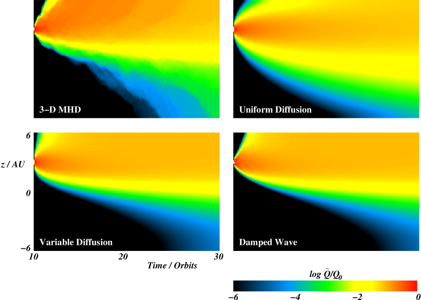
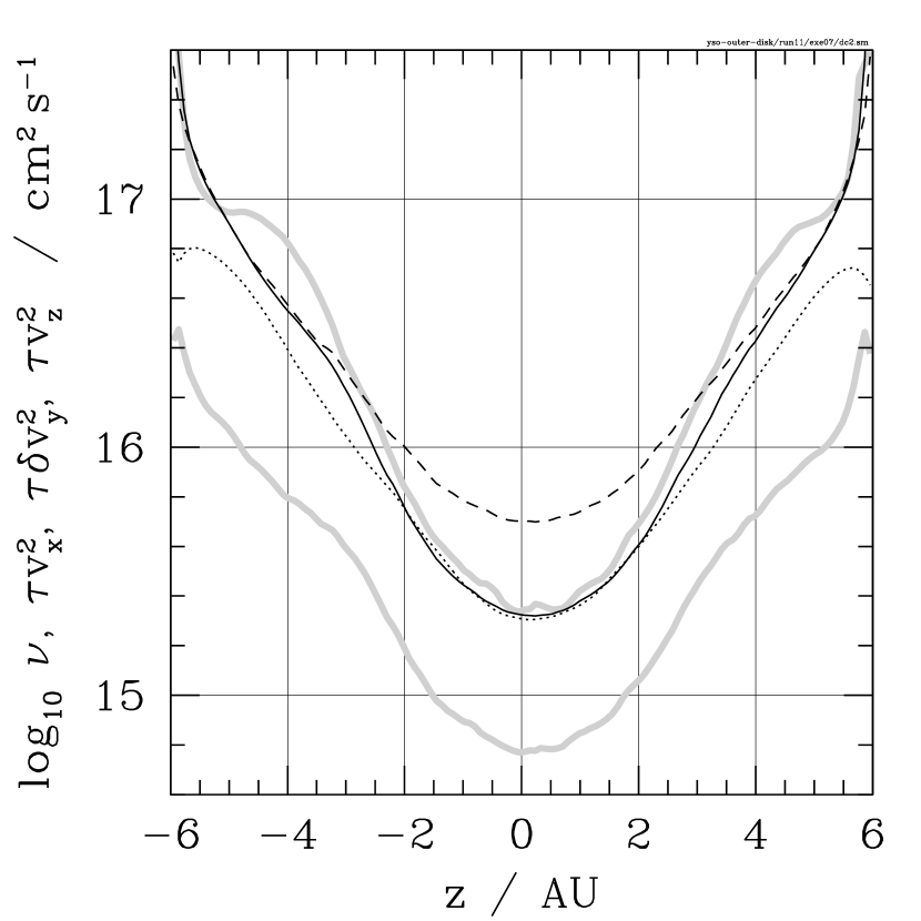
The two parameters in equation 11 are readily measured in the MHD calculation. The correlation time $\tau={\bar{F}_{z}}/(\overline{v_{z}{\bf v\cdot\nabla}q})$ between 10 and 30 orbits has a median value of 0.163 orbits, comparable to the shear time $(\frac{3}{2}\Omega)^{-1}=0.106$ orbits. The range of values is rather wide and is shown in figure 2. The RMS vertical speed $(\overline{v_{z}^{2}})^{1/2}$ ranges from 5% of the sound speed at the midplane to one-quarter the sound speed near the domain top and bottom, as shown in figure 3. Slower speeds within 0.5 AU of the boundaries are due to the restriction of the vertical movement by the no-inflow condition. Solutions of equation 11 using the measured coefficients are compared against the MHD spreading results in figure 4. Three cases are shown. The common practice in past chemical models is followed at top right, where the second time derivative term is neglected and the diffusion equation is solved with a uniform coefficient corresponding to the domain-averaged total accretion stress. At lower left, the diffusion coefficient $\tau{\overline{v_{z}^{2}}}$ is allowed to vary with height. At lower right, all the terms are included in the damped wave equation. The damped wave solution best matches the MHD results.

Figure 2: Histogram of turbulent correlation times $\tau$ measured in the MHD calculation between 10 and 30 orbits. The measurements are made every 0.1 orbits at each height on the computational grid. Zero correlation time, indicated by a vertical dashed line, occurs less often than small positive and negative values. The median correlation time is 0.163 orbits.

Figure 3: Density profile (top) and vertical velocity dispersion (bottom) in the MHD calculation. Both are averaged horizontally and over time from 10 to 30 orbits, and are plotted against height. The velocity dispersion is scaled using the isothermal sound speed $c_{s}$.

Figure 4: Horizontally-averaged contaminant concentration $\bar{Q}$ (colors) versus height and time in the MHD calculation (top left) and three models. The solution of the diffusion equation with uniform coefficient is shown at top right, the diffusion equation with height-dependent coefficient at bottom left, and the damped wave equation 11 at bottom right. In the uniform diffusion case the contaminant spreads too quickly in the interior and too slowly in the surface layers. In the variable diffusion case the contaminant spreads too quickly in the first few orbits. The best match is with the full damped wave solution.

4.1 Accretion and Mixing

To find whether the mixing driven by the MRI is faster or slower than the accretion, we compare the turbulent diffusion coefficients for mixing in the radial and vertical directions with the angular momentum transfer coefficient or kinematic viscosity corresponding to the stress,

$$\nu={w_{xy}\over\rho\left|{\partial\Omega/\partial\ln R}\right|}.$$ (12)

The radial mixing is examined using a version of the fiducial run with the contaminant placed initially in the middle third of the domain width, and distributed uniformly in height and along the orbit. Radial and vertical mixing occur together because the disk is stratified. As shown in figure 5, the mixing is quickest in the surface layers.

Figure 5: Spreading of a contaminant in the radial and vertical directions. A uniform layer perpendicular to the $x$-direction is placed in the turbulence at ten orbits. Snapshots of the azimuthally-averaged contaminant density are shown at six times. The fastest spreading is in the radial direction in the surface layers. After five orbits the remaining radial gradients are small. The vertical mixing and the compression of gas moving toward the midplane become the main effects. The gray scale is linear between zero (white) and the initial value (black).

The turbulent mixing and angular momentum transfer coefficients are plotted against height in figure 6. The results from the fiducial run have been averaged from 10 to 90 orbits, and the turbulent correlation times for the radial and azimuthal mixing are set equal to that measured for the vertical mixing. There is an overall height variation, with both accretion and mixing fastest in the outer layers of the disk where the velocity dispersion is greatest. The accretion time $R^{2}/\nu$ of three million years at the midplane is similar to the duration of the disk accretion phase in star formation (Strom et al., 1989, 1993; Haisch et al., 2001; Metchev et al., 2004), while the accretion time at a height of 4 AU is just $10^{5}$ yr.

Accretion and vertical mixing occur at similar rates near the midplane, while at heights of 4 AU the coefficient for radial angular momentum transfer is about twice that for vertical diffusion. The radial mixing is faster than the vertical at all heights, in agreement with the results shown in figure 5 and also consistent with the relative sizes of the velocity fluctuation components in the calculations by Miller & Stone (2000). The importance of uncorrelated velocity fluctuations for the mixing is shown by the large ratios of the diffusion coefficients to the kinematic viscosity corresponding to the hydrodynamic part of the accretion stress. The hydrodynamic stress results only from correlated fluctuations in the radial and azimuthal velocities.

Figure 6: Time- and horizontally-averaged angular momentum transfer and turbulent mixing coefficients versus height. Thick gray lines show the total kinematic viscosity corresponding to the accretion stress, $(\frac{3}{2}\Omega)^{-1}\langle-B_{x}B_{y}/4\pi\rho+v_{x}\delta v_{y}\rangle$ (upper), and the hydrodynamic part alone (lower). Thin black curves mark the turbulent diffusion coefficients for mixing in the radial (dashed), azimuthal (solid) and vertical directions (dotted). A coefficient $10^{16}$ cm²s^-1 corresponds to a radial mixing time of 0.64 Myr.

4.2 Effects of the Spatial Resolution and Boundaries

The dependence of the results on the grid resolution is explored using a version of the fiducial run with the number of zones along each axis doubled to $64\times 128\times 256$. Over twenty orbits, the time- and horizontally-averaged profiles of the accretion stress and mixing coefficient differ from the fiducial version by less than the range of time variation. Any sensitivity to the grid spacing is weak.

Possible effects of the vertical boundaries are checked by repeating the first thirty orbits of the fiducial calculation in a taller domain. The height and the number of grid zones in the vertical direction are increased by 25%, to 7.5 AU either side of the midplane and 160 zones. The resulting vertical profiles of the density, accretion stress, and mixing coefficient are similar where the two calculations overlap, except within 0.7 AU of the top and bottom boundaries. The time-averaged accretion stress at the boundaries of the fiducial calculation is up to twice that at the same height in the taller version, due to magnetic forces where field lines exit the domain. The mixing coefficient in the taller calculation increases smoothly with height through 6 AU, while in the fiducial run the mixing coefficient declines within 0.7 AU of the boundaries. We conclude that the mixing rates are affected by the boundaries only in the top and bottom 6% of the domain height. Solutions of equation 11 without the boundary effects can be obtained by projecting the approximately cubic height dependence of the diffusion coefficient from nearer the midplane.

The density floor is generally applied only in a few zones near the vertical boundaries. The application of the floor in the fiducial run between 10 and 30 orbits increases the mean density by less than one part in $10^{7}$. As a further check, a version of the taller calculation with the floor reduced tenfold to $10^{-19}$ g cm^-3 is run to twenty orbits. The mean profiles of the pressure, accretion stress and mixing coefficient are not significantly different from those above.

The effects of the radial box size are tested by repeating the first sixty orbits of the fiducial calculation in a box with the width and the number of grid zones in the radial direction doubled, so that there are $64\times 64\times 128$ zones. The horizontally-averaged accretion stress and velocity fluctuations are similar to those in the fiducial run.

4.3 Vertical Magnetic Fields

The calculations described above have zero net vertical magnetic flux. A mean vertical field leads to larger accretion stresses (Hawley, Gammie, & Balbus, 1995). The flow is dominated by the repeated formation and break-up of approximately axisymmetric pairs of inward and outward-moving layers, in unstratified shearing-box calculations with the MRI wavelength a few times shorter than the domain height (Sano & Inutsuka, 2001), while in stratified calculations, the strong magnetic fields in the layers disrupt the disk (Miller & Stone, 2000). A similar disruption occurs in a version of our fiducial run with the same uniform initial magnetic pressure but the field lines vertical throughout. The MRI reaches non-linear amplitudes at 2.5 orbits, strong radial and azimuthal fields are generated, the mean magnetic pressure exceeds the gas pressure at 2.9 orbits, the ram pressure of the velocity fluctuations is greater than the gas pressure after 3.6 orbits, and the calculation is halted as mass and magnetic fields are ejected rapidly through the top and bottom boundaries. The shearing-box approximation is unsuited to study vertical mixing in this situation. Disk annuli threaded by net vertical magnetic fields will be violently active and may be short-lived, if the MRI wavelength is similar to the disk thickness.

5 STEADY-STATE AND FLUCTUATIONS

In the final set of calculations we examine the distribution of the contaminant in the presence of fixed sources. The release of a molecular species into the gas phase in the disk surface layers is represented by holding the contaminant density fixed at its initial value in the top and bottom ten percent of the domain height. Two calculations are carried out starting at ten orbits, after the turbulence is well-established. In the first, the concentration is initially zero except in the surface-layer sources. The contaminant spreads gradually into the interior through the turbulent motions, and the midplane concentration increases with time. The compression of the gas moving from the surface layers to the midplane leads to midplane contaminant densities greater than the density at the source. The gas density at the midplane averages 59 times greater than at the inner edge of the source region, while after eighty orbits of mixing, the contaminant density at the midplane is 5.4 times that at the source and still increasing. The time for the interior to reach equilibrium with the source is clearly greater than the run length of $13\,000$ years. A rough estimate of the equilibration time is obtained using the distance from source to midplane and the turbulent diffusion coefficient at the midplane, where the mixing is slowest (figure 6). The result, $(4.8{\rm AU})^{2}/(\tau\overline{u_{z}^{2}}[z=0])=80\,000$ yr, is about six times the run duration.

In the second calculation with fixed sources, the contaminant density in the disk interior is initially set to the steady-state solution of the damped wave equation 11. The damped wave and diffusion equations have the same equilibrium solution since they differ only by a time-derivative term. The diffusion coefficient is obtained by averaging horizontally and over time in the previous MHD calculation. The horizontally-averaged profile of the contaminant remains near the steady-state solution for eighty orbits despite fluctuations in the mixing rate, as shown in figure 7. The midplane contaminant density varies around its starting point, with the largest value just 8% greater than the smallest, and the time average 25 times that at the source. The equilibrium contaminant concentration is least at the midplane, where the mixing is slowest.

Figure 7: The vertical profile of contaminant concentration (top panel), averaged over horizontal planes and over time (thick solid line), in the calculation starting with the steady-state solution of the damped wave equation 11. The initial state is marked by circles and the time variation is shown by the profiles at the times of lowest and highest midplane density, 10.4 and 54.6 orbits, respectively (thin solid lines). A vertical dashed line lies at the boundary of the source region where the contaminant density is fixed, and a horizontal dashed line shows the concentration at the source. In the bottom panel the diffusion coefficient is plotted against height (thick solid line). The coefficient is taken from the previous MHD calculation and is averaged horizontally as well as between the top and bottom halves of the domain and over time. Also shown are the horizontally-averaged profiles at 20, 40, 60 and 80 orbits (thin solid, dotted, dashed and long-dashed curves, respectively) together with the kinematic viscosity (thick horizontal dashed line) computed from the domain-averaged total accretion stress and the domain-averaged gas density.

While the horizontally-averaged profile remains near a steady state, large horizontal fluctuations in the contaminant density persist throughout the run, due to changes in the rate and direction of the turbulent transport. The largest contaminant density at a height of 4 AU is two to seven times greater than the smallest. The density range and its time variations are shown in figure 8. The variations occur over timescales from the turbulent correlation time up to the duration of the calculation. Variations of this kind are missing from hydrostatic models and are large enough to be important for the overall chemical evolution of protostellar disks.

Figure 8: Maximum, average and minimum contaminant densities on the horizontal surface 4 AU above the midplane, as functions of time in the MHD calculation near steady-state. The contrast is typically about a factor three. The densities are measured relative to the value in the source layers.

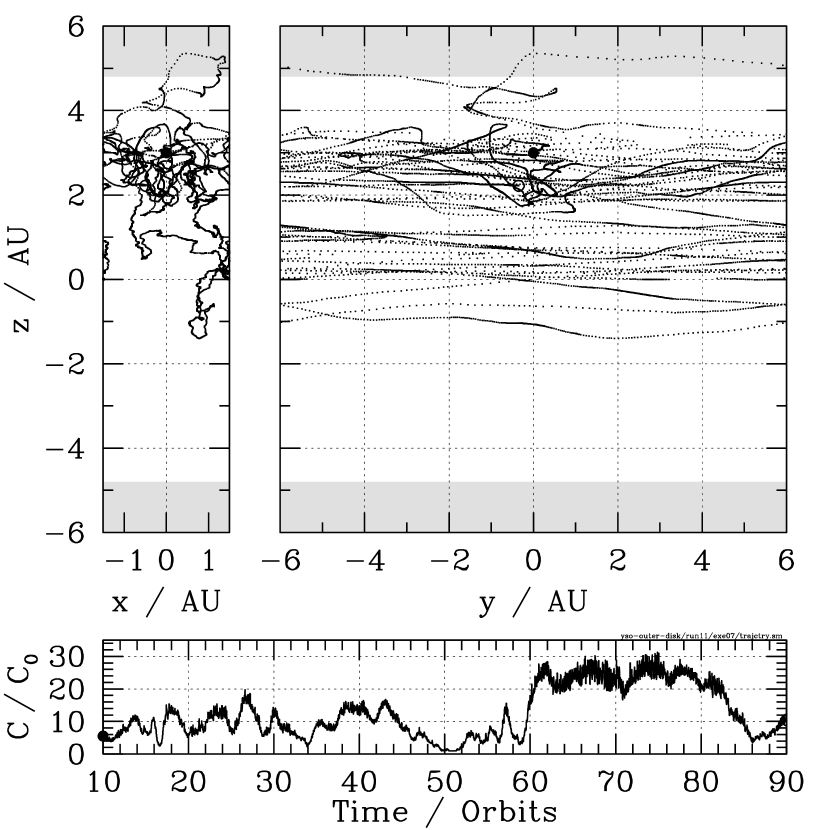
Individual fluid elements in the disk may pass through a wide range of environments on their paths through the turbulence. The chemical compositions of the fluid elements will reflect the histories of local conditions if the chemical reactions fail to reach equilibrium over the flow timescales. The history of a representative fluid element in the MHD calculation with the contaminant near steady-state is shown in figure 9. Over $13\,000$ years the element traverses the whole range of heights. The ambient contaminant density varies by around 20% on the turbulent correlation timescale of 30 years, and by factors of three over a few hundred years due to horizontal motions through fluctuations like those shown in figure 8. The density occasionally changes by an order of magnitude within a thousand years as the fluid element moves rapidly in height. Note that the path as viewed along the $x$-direction in the top right panel of figure 9 is broken where the element crosses the shearing-periodic radial boundary, leading to an offset along the $y$-direction. Paths like that in figure 9 will also be traced by dust grains that are well-coupled to the gas by drag forces.

Figure 9: Trajectory of a fluid element in the turbulence, projected onto the $x-z$ plane (top left) and the $y-z$ plane (top right). The element lies 3 AU above the origin at 10 orbits (filled circles) and follows a path that takes it into the upper contaminant source layer (gray) and across the midplane, and at 90 orbits (open circles) returns near the original location. The time history of the local contaminant density is plotted in the bottom panel.

6 SUMMARY AND CONCLUSIONS

We have followed the mixing of a passive trace species and the trajectories of individual fluid elements in the outer Solar nebula, using 3-D MHD calculations. A small patch of the nebula centered at a radius of 30 AU is modeled in the shearing-box approximation, with the vertical component of the gravity of the young Sun included. The mixing is caused by the turbulence driven by the magneto-rotational instability. The magnetic and hydrodynamic stresses in the turbulence correspond to a kinematic accretion viscosity that is greatest in the surface layers because of (1) the density stratification and (2) the stronger magnetic fields in the surface layers. The mixing along the vertical direction is well-matched by the solutions of a one-dimensional damped wave equation, with damping coefficient approximately the product of the shear time and the mean squared vertical turbulent speed. A similar horizontally-averaged diffusion description of the mixing without the wave term gives a poorer fit to the MHD results: the contaminant spreads faster than the RMS turbulent speed at early times, owing to the infinite signal propagation speeds that occur generically in solutions of the diffusion equation. The horizontal averaging used in both the damped wave and diffusion pictures glosses over some details of the flow that could affect the chemical evolution. The contaminant density in the MHD calculations varies substantially across horizontal planes at any given time, due to fluctuations in the speed and direction of the gas flows. The mixing caused by the turbulence is erratic, and can be expected to intermittently force the nebula away from local chemical equilibrium. Also, individual fluid elements sometimes move between the interior and the surface layers in a small fraction of the time needed to reach an overall mixing equilibrium. However an improvement over existing one-dimensional treatments of vertical mixing can be obtained by solving equation 11.

The measured vertical mixing coefficient varies with height in a similar way to the angular momentum transfer coefficient. The two are equal at the midplane, while at 4 AU the mixing coefficient is about half the local kinematic viscosity, so that the Schmidt number ranges from one to two. The accretion time in the midplane is three million years, comparable to the lifetimes of the disks around T Tauri stars. The accretion time in the surface layers is less than $10^{5}$ yr, and similar to the timescale for vertical mixing to the midplane. The transport times suggest a picture in which the fastest way to move midplane material from one radius to another is by first mixing it out to the surface layers. In this scenario, only the solid particles small enough to be suspended in the low-density surface-layer gas are carried efficiently. Larger bodies remain near the midplane where both accretion and mixing are slow. Such fast surface-layer transfer could lead to size-dependent composition differences among primordial dust grains and could affect the molecular abundances in the region where the giant planets formed. The height dependence of the mixing rate means that concentration gradients persist even in the steady state. The stratification of the turbulence may also be significant for grain growth. The RMS velocity fluctuations increase with height, exceeding 100 m s^-1 above 4 AU. Aggregate icy grains can be broken apart in impacts at these speeds (Dominik & Tielens, 1997), while bodies that settle near the midplane will experience mostly slower collisions leading to compaction or sticking. The vertical mixing may lie behind the difference in HCN deuterium fraction between comets and the interstellar medium. Molecules formed in the surface layers of the nebula, where warm temperatures led to lower deuteration, could have been incorporated into bodies assembled near the midplane. There is a need for grain growth and chemical evolution calculations that include the effects of both radial and vertical transport.

References

- Aikawa et al. (2002) Aikawa, Y., van Zadelhoff, G. J., van Dishoeck, E. F., & Herbst, E. 2002, A&A, 386, 622
- Balbus & Hawley (1991) Balbus, S. A., & Hawley, J. F. 1991, ApJ, 376, 214
- Balbus & Hawley (1998) Balbus, S. A., & Hawley, J. F. 1998, Rev. Mod. Phys. 70, 1
- Bar-Nun et al. (1988) Bar-Nun, A., Kleinfeld, I., & Kochavi, E. 1988, Phys. Rev. B, 38, 7749
- Blackman & Field (2003) Blackman, E. G., & Field, G. B. 2003, Phys. of Fluids, 15, L73
- Brandenburg et al. (2004) Brandenburg, A., Käpylä, P. J., & Mohammed, A. 2004, Phys. of Fluids, 16, 1020
- Carballido et al. (2005) Carballido, A., Stone, J. M., & Pringle, J. E. 2005, MNRAS, 358, 1055
- Ceccarelli & Dominik (2005) Ceccarelli, C., & Dominik, C. 2005, A&A, 440, 583
- Chiang & Goldreich (1997) Chiang, E. I., & Goldreich, P. 1997, ApJ, 490, 368
- Cisowski & Hood (1991) Cisowski, S. M., & Hood, L. L. 1991, in The Sun in Time (Tucson: University of Arizona Press), 761
- Cotera et al. (2001) Cotera, A. S., et al. 2001, ApJ, 556, 958
- D’Alessio et al. (2001) D’Alessio, P., Calvet, N., & Hartmann, L. 2001, ApJ, 553, 321
- Dominik & Tielens (1997) Dominik, C., & Tielens, A. G. G. M. 1997, ApJ, 480, 647
- Draine & Lee (1984) Draine, B. T., & Lee, H. M. 1984, ApJ, 285, 89
- Dullemond & Dominik (2005) Dullemond, C. P., & Dominik, C. 2005, A&A, 434, 971
- Gail (2001) Gail, H.-P. 2001, A&A, 378, 192
- Haisch et al. (2001) Haisch, K. E., Lada, E. A., & Lada, C. J. 2001, ApJ, 553, 153
- Hawley, Gammie, & Balbus (1995) Hawley, J. F., Gammie, C. F., & Balbus, S. A. 1995, ApJ, 440, 742
- Hawley & Stone (1995) Hawley, J. F., & Stone, J. M. 1995, Comp. Phys. Comm., 89, 127
- Hawley & Stone (1998) Hawley, J. F., & Stone, J. M. 1998, ApJ, 501, 758
- Hersant et al. (2004) Hersant, F., Gautier, D., & Lunine, J. I. 2004, Planetary & Space Sci. 52, 623
- Ilgner et al. (2004) Ilgner, M., Henning, Th., Markwick, A. J., & Millar, T. J. 2004, A&A, 415, 643
- Ilgner & Nelson (2005) Ilgner, M., & Nelson, R. P. 2005, astro-ph/0509553
- Johansen & Klahr (2005) Johansen, A., & Klahr, H. 2005, astro-ph/0501641
- Lunine & Stevenson (1985) Lunine, J. I., & Stevenson, D. J. 1985, ApJS, 58, 493
- Lunine et al. (2000) Lunine, J. I., Owen, T. C., & Brown, R. H. 2000, in: Mannings V., Boss A. & Russell S. S., Editors, 2000. Protostars and Planets IV (Univ. of Arizona Press: Tucson), 1055
- McCabe et al. (2003) McCabe, C., Duchêne, G. & Ghez, A. M. 2003, ApJ, 588, L113
- Metchev et al. (2004) Metchev, S. A., Hillenbrand, L. A., & Meyer, M. R. 2004, ApJ, 600, 435
- Miller & Stone (2000) Miller, K. A., & Stone, J. M. 2000, ApJ, 534, 398
- Morfill & Völk (1984) Morfill, G. E., & Völk, H. J. 1984, ApJ, 287, 371
- Salmeron & Wardle (2005) Salmeron, R., & Wardle, M. 2005, MNRAS, 361, 45
- Sano & Inutsuka (2001) Sano, T., & Inutsuka, S. 2001, ApJ, 561, L179
- Sano et al. (2000) Sano, T., Miyama, S. M., Umebayashi, T., & Nakano, T. 2000, ApJ, 543, 486
- Sano & Stone (2002a) Sano, T., & Stone, J. M. 2002a, ApJ, 570, 314
- Sano & Stone (2002b) Sano, T., & Stone, J. M. 2002b, ApJ, 577, 534
- Shuping et al. (2003) Shuping, R. Y., Bally, J., Morris, M., & Throop, H. 2003, ApJ, 587, L109
- Stevenson (1990) Stevenson, D. J. 1990, ApJ, 348, 730
- Stone & Norman (1992a) Stone, J. M., & Norman, M. L. 1992a, ApJS, 80, 753
- Stone & Norman (1992b) Stone, J. M., & Norman, M. L. 1992b, ApJS, 80, 791
- Strom et al. (1989) Strom, K. M., Strom, S. E., Edwards, S., Cabrit, S., & Skrutskie, M. F. 1989, AJ, 97, 1451
- Strom et al. (1993) Strom, S. E., Edwards, S., & Skrutskie, M. F. 1993, in: Levy, E. H., & Lunine, J. I., Editors, 1993. Protostars and Planets III (Univ. of Arizona Press: Tucson), 837
- Suttner & Yorke (2001) Suttner, G., & Yorke, H. W. 2001, ApJ, 551, 461
- Tamura et al. (1999) Tamura, M., Hough, J. H., Greaves, J. S., Morino, J.-I., Chrysostomou, A., Holland, W. S., & Momose, M. 1999, ApJ, 525, 832
- Troland et al. (1996) Troland, T. H., Crutcher, R. M., Goodman, A. A., Heiles, C., Kazès, I., & Myers, P. C. 1996, ApJ, 471, 302
- Wardle & Ng (1999) Wardle, M., & Ng, C. 1999, MNRAS, 303, 239
- Willacy & Langer (2000) Willacy, K., & Langer, W. D. 2000, ApJ, 544, 903
- Willacy et al. (2006) Willacy, K., Langer, W. D., & Allen, M. A. 2006, ApJ, submitted
- Winters et al. (2003) Winters, W. F., Balbus, S. A. & Hawley, J. F. 2003, MNRAS, 340, 519
- Wooden et al. (1999) Wooden, D. H., Harker, D. E., Woodward, C. E., Butner, H. M., Koike, C., Witteborn, F. C. & McMurtry, C. W. 1999, ApJ, 517, 1034
- Young (2003) Young, R. E. 2003, New Astronomy Reviews, 47, 1