A New Time-Symmetric Block Time-Step Algorithm for N-Body Simulations

Abstract

Time-symmetric integration schemes share with symplectic schemes the property that their energy errors show a much better behavior than is the case for generic integration schemes. Allowing adaptive time steps typically leads to a loss of symplecticity. In contrast, time symmetry can be easily maintained, at least for a continuous choice of time step size. In large-scale N-body simulations, however, one often uses block time steps, where all time steps are forced to take on values as powers of two. This greatly facilitates parallelization, and hence code efficiency. Straightforward implementation of time-symmetry, translated to block time steps, faces significant hurdles. For example, iteration can lead to oscillatory behavior, and even when such behavior is suppressed, energy errors show a linear drift in time. We present an approach that circumvents these problems.

1 Introduction

For long-term N-body simulations, it is essential that the drift in the values of conserved quantities is kept to a minimum. The total energy is often used as an indicator of such a drift. During the last fifteen years, two approaches have been put forward to improve numerical conservation of energy and other theoretically conserved quantities: symplectic integration schemes, where the simulated system is guaranteed to follow a slightly perturbed Hamiltonian system, and time-symmetric integration schemes, where the simulated system follows the same trajectory in phase space, when run backwards or forwards

In both cases, for symplectic as well as for time-symmetric schemes, the introduction of adaptive time steps tends to destroy the desired properties. Symplectic schemes are perturbed to different Hamiltonians at different choices of time step length, and therefore lose their global symplecticity. Time-symmetric schemes typically determine their time step length at the beginning of a step, which implies that running a step backwards gives a slightly different length for that step. See Leimkuhler & Reich (2005) for a recent review of various attempts to remedy this situation.

In practice, many large-scale simulations in stellar dynamics use a block time-step approach, where the only allowed values for the time step length are powers of two (Aarseth, 2003). The name derives from the fact that, with this recipe, many particles will share the same step size, which implies that their orbit integration can be performed in parallel. An added benefit, in the case of individual time steps, is the fact that block time steps allow one to predict the positions of all particles only once per block time step, rather than separately for each particle that needs to be moved forward. Since parallelization is rapidly becoming essential for any major simulation, we explore in this paper the possibility to extend time symmetry to the use of block time steps.

In Section 2, we analyze some of the problems that occur when applying existing methods to the case of block time steps, and we offer a novel solution, with a truly time symmetric choice of time step, with the restriction that we only allow changes of a factor two in the direction of increasing and decreasing the time step. In Section 3, we present numerical tests of our new scheme, which show the superiority of our approach over various alternatives. Section 4 sums up.

2 Block Time Steps

2.1 Implicit Iterative Time Symmetrization

It is surprisingly easy to introduce a time-symmetric version for any adaptive self-starting integration scheme. Let $\xi=(r,v)$ be the $2N$-dimensional phase space vector for a system with $N$ degrees of freedom, and let $f(\xi_{i},\delta t_{i})$ be the operator that maps the phase space vector of the system at time $t_{i}$ to a new phase space vector at time $t_{i+1}=t_{i}+\delta t_{i}$. Any choice of self-starting integration scheme, together with a recipe to determine the next time step $\delta t_{i}$, at time $t_{i}$ and phase space value $\xi_{i}(t_{i})$, defines the precise form of $f(\xi_{i},\delta t_{i})$.

The recipe for making any such scheme time-symmetric was given by Hut, Makino & McMillan (1995), as:

$$\left\{\begin{array}[]{lcl}\xi_{i+1}&=&f(\xi_{i},\delta t_{i}),\\ \phantom{1}&\phantom{1}&\phantom{1}\\ \delta t_{i}&=&{\displaystyle\frac{h(\xi_{i})+h(\xi_{i+1})}{2}}\end{array}\right.$$ (1)

where $h(\xi)$ can be any time step criterion. Note that this recipe leads to an implicit integration scheme, which can be solved most easily through iteration. In practice, one or two iterations suffice to get excellent accuracy, but at the cost of doubling or tripling the number of force calculations that need to be performed. Extensions of this implicit symmetrization idea have been presented by Funato et al. (1996) and Hut et al. (1997).

Since we will need to inspect the idea of iteration below in more detail, let us write out the process here explicitly. We start with the given state $\xi_{i}$ and the implicit equation for $\xi_{i+1}$ of the form

$$\xi_{i+1}=f(\xi_{i},\delta t_{i}(\xi_{i},\xi_{i+1}))$$ (2)

The first guess for $\xi_{i+1}$ is

$$\xi_{i+1}^{(0)}=f(\xi_{i},\delta t_{i}(\xi_{i},\xi_{i}))$$ (3)

and we can consider this as our zeroth-order iteration. With this guess in hand, we can now start to iterate, finding

$$\xi_{i+1}^{(1)}=f(\xi_{i},\delta t_{i}(\xi_{i},\xi_{i+1}^{(0)}))$$ (4)

as our first-order iteration. This will already be much closer to the final value, as long as the time steps are small enough and the function $\delta t_{i}$ does not fluctuate too rapidly. In general, the $k^{th}$ iteration will yield a value for $\xi_{i+1}$ of

$$\xi_{i+1}^{(k)}=f(\xi_{i},\delta t_{i}(\xi_{i},\xi_{i+1}^{(k-1)}))$$ (5)

We will now consider the application of these techniques to block time steps. For the purpose of illustrating the use of block time steps, it will suffice to use the leapfrog scheme (also known as the Verlet-Störmer-Delambre scheme, according to the authors who rediscovered this scheme at roughly century-long intervals), which we present here in a self-starting, but still time-symmetric form:

$$r_{i+1} = r_{i}+v_{i}\delta t+a_{i}(\delta t)^{2}/2$$

$$v_{i+1} = v_{i}+(a_{i}+a_{i+1})\delta t/2$$ (6)

2.2 Flip-Flop Problem

To start with, we apply the recipe of Hut, Makino & McMillan (1995) to block time steps. Let us define a block time step at level $n$ as having a length:

$$\Delta t_{n}=\frac{\Delta t_{1}}{2^{n-1}}.$$ (7)

where $\Delta t_{1}$ is the maximum time step length. Starting with the continuum choice of

$$\delta t_{c,i}=\frac{h(\xi_{i})+h(\xi_{i+1})}{2}$$ (8)

we now force each time step to take on the block value $\delta t_{i}=\Delta t_{n}$ for the smallest $n$ value that obeys the condition $\Delta t_{n}\leq\delta t_{c,i}$. In more formal terms, $\delta t_{i}=\delta t_{i}(\delta t_{c,i})=\Delta t_{n}$ for the unique $n$ value for which

$$n=\min_{k\geq 1}\left\{k\ \Big{|}\ \frac{1}{2^{k-1}}\leq\frac{h(\xi_{i})+h(\xi_{i+1})}{2}\right\}$$ (9)

The problem with this approach is that we are no longer guaranteed to find convergence for our iteration process, as can be seen from the following example. Let $h(\xi_{i})=0.502$ and let the time derivative of $h(\xi_{i}(t))$ along the orbit be $(d/dt)h(\xi_{i}(t))=-0.01$. We then get the following results for our attempt at iteration.

$$\xi_{i+1}^{(0)} = f(\xi_{i},\delta t_{i}(\xi_{i},\xi_{i}))=f(\xi_{i},\delta t_{i}(h(\xi_{i})))$$ (10)

$$= f(\xi_{i},\delta t_{i}(0.502))=f(\xi_{i},0.5)$$

$$\xi_{i+1}^{(1)} = f(\xi_{i},\delta t_{i}(\xi_{i},\xi_{i+1}^{0}))=f(\xi_{i},\delta t_{i}([h(\xi_{i})+h(\xi_{i+1}^{0})]/2))$$ (11)

$$= f(\xi_{i},\delta t_{i}([0.502+(0.502+0.5*(-0.01))]/2))$$

$$= f(\xi_{i},\delta t_{i}([0.502+0.497]/2))$$

$$= f(\xi_{i},\delta t_{i}(0.4995))=f(\xi_{i},0.25)$$

$$\xi_{i+1}^{(2)} = f(\xi_{i},\delta t_{i}(\xi_{i},\xi_{i+1}^{1}))=f(\xi_{i},\delta t_{i}([h(\xi_{i})+h(\xi_{i+1}^{1})]/2))$$ (12)

$$= f(\xi_{i},\delta t_{i}([0.502+(0.502+0.25*(-0.01))]/2))$$

$$= f(\xi_{i},\delta t_{i}([0.502+0.4995]/2))$$

$$= f(\xi_{i},\delta t_{i}(0.50075))=f(\xi_{i},0.5)$$

And from here on, $\xi_{i+1}^{(k)}=f(\xi_{i},0.25)$ for every odd value of $k$ and $\xi_{i+1}^{(k)}=f(\xi_{i},0.5)$ for every even value of $k$: the process of iteration will never converge.

Under realistic conditions, for slowly varying $h$ functions and small time steps, this flip-flop behavior will not occur often, but it will occur sometimes, for a non-negligible fraction of the time. We can see this already from the above example: for a linear decrease in the $h$ function of $(d/dt)h(\xi_{i}(t))=-0.01$, we will get flip-flopping not only for $h(\xi_{i})=0.502$ but for any value in the finite range $0.50125<h(\xi_{i})<0.5025$.

Since iteration converges correctly over the rest of the interval $0.5<h(\xi_{i})<1$, we conclude that in this particular case flip-flopping occurs about one quarter of one percent of the time, over this interval. This is far too frequent to be negligible in a realistic situation.

Clearly, a straightforward extension of the implicit iterative time symmetrization approach does not work for block time steps, because iteration does not converge. We have to add some feature, in some way. Our first attempt at a solution is to take the smallest of the two values in a flip-flop situation.

2.3 Flip-Flop Resolution

The most straightforward solution of the flip-flop dilemma is like cutting the Gordian knot: we just take the lowest value of the two alternate states. The drawback of this solution is that in general we need at least two iterations for each time step, to make sure that we have spotted, and then correctly treated, all flip-flop situation. In general, it is only at the third iteration that it becomes obvious that a flip-flop is occurring. To see this, consider the previous example with a starting value of $h(\xi_{i})=0.501$. In that case we will get $\xi_{i+1}^{(0)}=f(\xi_{i},0.5)$ and $\xi_{i+1}^{(1)}=f(\xi_{i},0.25)$, just as when we started with $h(\xi_{i})=0.502$. The difference shows up only at the second iteration, where we now find $\xi_{i+1}^{(2)}=f(\xi_{i},0.25)$, a value that will hold for all higher iterations as well.

The original iterative approach to time symmetry in practice already gives good results when we use only one iteration. This implies a penalty, in terms of force calculations per time steps, of a factor two compared to non-time-symmetric explicit integration. Now the use of flip-flop resolution will force us to always take at least two iterations per step, raising the penalty to become at least a factor of three.

However, there is a more serious problem: there is still no guarantee that taking the lowest value in a flip-flop situation leads to a time-symmetric recipe. In fact, what is even more important, we have not yet checked whether our symmetric block time-step scheme is really time symmetric, in the absence of flip-flop complications.

In order to investigate these questions, let us return to the example we used above, but instead of a linear time derivative, let us now use a quadratic time derivative for the $h$ function that gives the estimate for the time step size. Rather than writing a formal definition, let us just state the values, while shifting the time scale so that $t=0$ coincides with the particle position being $\xi_{i}$:

$$h(0.00) = 0.502$$

$$h(0.25) = 0.499$$

$$h(0.50) = 0.499$$ (13)

When we start at time $t=0$, and we integrate forwards. we find:

$$\xi_{i+1}^{(0)} = f(\xi_{i},\delta t_{i}(\xi_{i},\xi_{i}))=f(\xi_{i},\delta t_{i}(h(\xi_{i})))$$ (14)

$$= f(\xi_{i},\delta t_{i}(0.502))=f(\xi_{i},0.5)$$

$$\xi_{i+1}^{(1)} = f(\xi_{i},\delta t_{i}(\xi_{i},\xi_{i+1}^{0}))=f(\xi_{i},\delta t_{i}([h(\xi_{i})+h(\xi_{i+1}^{0})]/2))$$ (15)

$$= f(\xi_{i},\delta t_{i}([0.502+0.499]/2))$$

$$= f(\xi_{i},\delta t_{i}(0.5005))=f(\xi_{i},0.5)$$

and so on: all further $k$th iterations will result in $\xi_{i+k}^{(1)}=f(\xi_{i},0.5)$. There is no flip-flop situation, when moving forward in time.

However, when we now turn the clock backward, after taking this step of half a time unit, we start with the value $h(0.50)=0.499$, which leads to a first step back of $\delta t=0.25$. The end point of the first step back is $t=0.25$ with $h(0.25)=0.499$. Therefore, also here there is no flip-flop situation: all iterations, while going backward, result in a time step size of $\delta t=0.25$.

We have thus constructed a counter example, where forward integration would proceed with time step $\delta t=0.5$ and subsequent backward integration would proceed with time step $\delta t=0.25$. Clearly, our scheme is not yet time symmetric, even in the absence of a flip-flop case.

2.4 A First Attempt at a Solution

Let us rethink the whole procedure. The basic problem has been that the very first step in any of our algorithms proposed so far has not been time symmetric. The very first step moves forward, and leads to a newly evolved system at the end of the first step. Only after making such a trial integration, do we look back, and try to restore symmetry. However, as we have seen, the danger is large that this trial integration is not exhaustive: it may already go too far, or not far enough, and thereby it may simply overlook a type of move that the same algorithm would make if we would start out in the time-reversed direction.

Formulating the problem in this way, immediately suggests a solution. At any point in time, let us first try to make the largest step that is allowed. If that step turns out to be too large for our algorithm, we try a step that is half that size. if that step is too large still, we again half the size, and so on, until we find a step size that agrees with our algorithm, when evaluated in both time directions. A similar treatment has been described by Quin et al (1997).

This type of approach is clearly more symmetric than what we have attempted so far. Instead of using information of the physical system at the starting point of the next integration step, we only use a mathematical criterion to find the largest time step size allowed at that point, and we then apply the physical criteria symmetrically in both directions.

Let us give an example. If the largest time step size is chosen to be unity, then at time $t=0$ we start by considering this time step. We try, in this order $\delta t=1$, $\delta t=0.5$, $\delta t=0.25$, and so on, until we find a time step for which integration starting in the forward direction, and integration starting in the backward direction, both result in the new time step being acceptable. Let us say that this is the case for $\delta t=0.125$.

After taking this step, we are at time $t=0.125$. The largest time step allowed at that point, forward or backward, is $\delta t=0.125$. Any larger time step would result in non-alignment of the block time steps: in the backward direction it would jump over $t=0$. So at this point we start by considering once more $\delta t=0.125$. If that time step is too large, we try half that time step, halving it successively until we find a satisfactory time step size.

Imagine that the second time step size is also $\delta t=0.125$. In that case, we land at $t=0.25$. From there on, the maximum allowed time step size is $\delta t=0.25$, so the first try should be that size.

In principle, this approach seems to be really time symmetric. However, there is a huge problem with this type of scheme, as we have just formulated it. Imagine the system to crawl along with time steps of, say $\delta t=1/1024$, and reaching time $t=1$. Our new recipe then suggests to start by trying $\delta t=1$, a 1024-fold increase in time step! Whatever subtle physical effect it was that forced us to take such small time steps, is completely ignored by the mathematical recipe that forces us to look at such a ridiculously large time step.

For example, in the case of stellar dynamics, a double star may force the stars that orbit each other to take time steps that are necessarily far shorter than the orbital period. Starting out with a trial step size that is far larger than an orbital period may or may not give spuriously safe-looking results. Clearly, we have to exclude such enormous jumps in time step.

2.5 A Second Attempt at a Solution

The simplest solution to taming sudden unphysical increases in time steps is to allow at most an increase of a factor two, in either the forward or the backward direction. This then implies that we can only allow decreases of a factor two, and not more than two, in either direction. The reason is that a decrease of a factor four in one direction in time would automatically translate into an increase of a factor four in the other direction.

Note that we have to be careful with our time step criterion. If we allow time steps that are too large, we may encounter situations where our time step criterion would suggest us to shrink time steps by a factor of four, from one step to the other. Since our algorithm does not allow this, we can at most shrink by a factor of two, which may imply an unacceptably large step. However, if our time step criterion is sufficiently strict, allowing only reasonably small time steps too start with, it will be able to resolve the gradients in the criterion in such as way as to handle all changes gracefully through halving and doubling.

When we apply this restriction to the scheme outlined in the previous subsection, we arrive at the following compact algorithm.

First a matter of notation. Any block time step, of size $\delta t=1/2^{k}$, connects two points in time, only one of which can be written at $t=Z/2^{(k-1)}$, with $Z$ an integer. Let us call that time value an even time, from the point of view of the given time step size, and let us call that other time value an odd time. To give an example, if $\delta t=0.125$, than $t=0,0.25,0.5,0.75,1$ are all even times, while $t=0.125,0.375,0.625,0.875$ are all odd times.

Here is our algorithm:

• When we start in a given direction in time, at a given point in time, we should determine the time step size of the last step made by the system. In that way, we can determine whether the current time is even or odd, with respect to that last time step.

• If the current time is odd, our one and only choice is: to continue with the same size time step, or to halve the time step. First, we try to continue with the same time step. If, upon iteration, that time step qualifies according to the time-symmetry criterion used before, Eq. 9, we continue to use the same time step size as was used in the previous time step. If not, we use half of the previous time step.

• If the current time step is even, we have a choice between three options for the new time step size: doubling the previous time step size, keeping it the same, or halving it. We first try the largest value, given by doubling. If Eq.9 shows us that this larger time step is not too large, we accept it, otherwise we consider keeping the time step size the same. If Eq.9 shows us that keeping the time step size the same is okay, we accept that choice, otherwise we just halve the time step, in which case no further testing is needed.

Note that in this scheme, we always start with the largest possible candidate value for the time step size. Subsequently, we may consider smaller values, but the direction of consideration is always from larger to smaller, never from smaller to larger. This guarantees that we do not run into the flip-flop problem mentioned above.

3 Numerical Tests

We present here the results for a gravitational two-body integration. The relative orbit of the two point masses forms an ellipse with an eccentricity of $e=0.99$. We have chosen a time unit such that the period of the orbit is $T=2\pi$.

We have implemented four different integration schemes:

0) the original time-symmetric integration scheme described by Hut, Makino & McMillan (1995), where there is a continuous choice of time step size. This is the approach described in section 2.1. We have used five iterations for each step.

1) a block-time-step generalization, with a fixed number of iterations. This is the approach analyzed in section 2.2. Here, too, we chose five iterations for each step.

2) a block time step generalization, with a variable number of iterations. If after five iterations, the fourth and the fifth iterations still give a different block time step size, then we choose the smallest of the two. This recipe avoids flip-flop situations. It is the approach described in section 2.3.

The algorithm described in the next section, 2.4, we have not implemented here, because it is guaranteed to lead to large errors in those cases where a new large time step is allowed again just before pericenter passage. We therefore switched directly to the following section:

3) the implementation of our favorite algorithm, where we start with a truly time symmetric choice of time step, with the restrictions that we only allow changes of a factor two in the direction of increasing and decreasing the time step, and that we only allow an increase of time step on the so-called even time boundaries. This is the approach given in section 2.5.

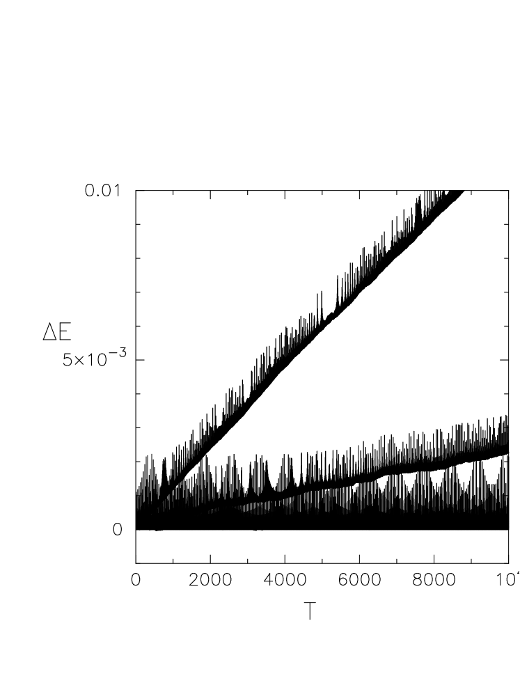
Figure 1: Energy errors for a two-body integration of a bound orbit with eccentricity $e=0.99$. The top line with highest slope corresponds to algorithm 1, the line with intermediate slope corresponds to algorithm 2, and below those the two lines for algorithms 0 and 3 are indistinguishable in this figure.

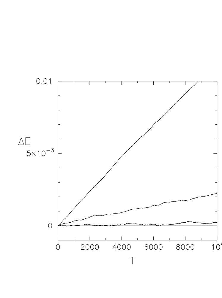
Figure 2: The energy errors at apocenter. The four lines, from top to bottom, correspond to algorithms 1, 2, 3, and 0.

In figures 1 and 2 we show the results of integrating our highly eccentric binary with these four integration schemes. In each case, the largest errors are produced by algorithm 1), smaller errors are produced by algorithm 2), and even smaller errors appear with algorithm 3). Finally, algorithm 0) gives the smallest errors.

Figure 1 shows the energy error in the two-body integration as a function of time. As is generally the case for time-symmetric integration, the errors that occur during one orbit are far larger than the systematic error that is generated during a full orbit. To bring this out more clearly, figure 2 shows the error only one time per orbit, at apocenter, the point in the orbit where the two particles are separated furthest from each other, and the error is the smallest.

Finally, figure 3 shows the same data as figure 2, but for a period of time that is ten times longer. In both figures 2 and 3, it is clear that the first two block time steps algorithms, 1) and 2), both show a linear drift in energy. This is a clear sign of the fact that they violate time symmetry. Note that in both figures algorithm 3) gives rise to a time dependency that looks like a random walk. This may well be the best that can be done with block time steps, when we require time symmetry.

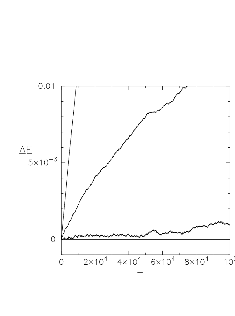
Figure 3: Same as Fig. 2, but for a duration that is ten times longer.

4 Summary

To sum up, we have succeeded in constructing an algorithm for time symmetrizing block time steps that does not show a linear growth of energy errors. As far as we know, this is the first such algorithm that has been discovered. We expect this algorithm to have practical value for a wide range of large-scale parallel N-body simulations.

We acknowledge conversations with Joachim Stadel at the IPAM workshop on N-Body Problems in Astrophysics, in April 2005, where he presented a time symmetric version of the preprint by Quinn et al. (1997) which is similar to our first attempt at a solution, described in section 2.4. See also his PhD thesis, available as “www-theorie.physik.unizh.ch/~stadel/downloads/thesis.ps”. M.K. and H.S. acknowledge research support from ITU-Sun CEAET grant 5009-2003-03. P.H. thanks Prof. Ninomiya for his kind hospitality at the Yukawa Institute at Kyoto University, through the Grants-in-Aid for Scientific Research on Priority Areas, number 763, “Dynamics of Strings and Fields”, from the Ministry of Education, Culture, Sports, Science and Technology, Japan.

References

- (1)
- Aarseth (2003) Aarseth, J., S., 2003, Gravitational N-Body Simulations, Cambridge University Press.
- Hut et al. (1997) Hut, P., Funato, Y., Kokubo, E., Makino, J. & McMillan, S., 1997, Time Symmetrization Meta-Algorithms, in Computational Astrophysics, eds. D. A. Clarke and M. J. West, ASP Conference Series, Vol. 123 (San Francisco: ASP), pp. 26-31.
- Funato et al. (1996) Funato, Y., Hut, P., McMillan, S. & Makino, J., 1996, Time-Symmetrized Kustaanheimo-Stiefel Regularization, Astron. J. 112, 1697-1708.
- Hut, Makino & McMillan (1995) Hut, P., Makino, J. & McMillan, S., 1995, Building A Better Leapfrog, Astrophysical Journal 443, L93-L96.
- Leimkuhler & Reich (2005) Leimkuhler, B. & Reich, S., 2005, Simulating Hamiltonian Dynamics, Cambridge University Press.
- Makino (1991) Makino, J., 1991, Optimal Order and Time-Step Criterion for Aarseth-Type N-body Integrations, Astrophysical Journal 369, 200-212.
- Quinn et al. (1997) Quinn, T., Katz, N., Stadel, J. & Lake, G., 1997, Time stepping N-body simulations, preprint, archived on http://arxiv.org/ps/astro-ph/9710043.