Variations in the spectral slope of Sgr A* during a NIR flare

Abstract

We have observed a bright flare of Sgr A* in the near infrared with the adaptive optics assisted integral field spectrometer SINFONI. Within the uncertainties, the observed spectrum is featureless and can be described by a power law. Our data suggest that the spectral index is correlated with the instantaneous flux and that both quantities experience significant changes within less than one hour. We argue that the near infrared flares from Sgr A* are due to synchrotron emission of transiently heated electrons, the emission being affected by orbital dynamics and synchrotron cooling, both acting on timescales of $\approx 20$ minutes.

1. Introduction

The detection of stellar orbits (Schödel et al., 2002; Eisenhauer et al., 2005; Ghez et al., 2003, 2005a) close to Sgr A* has proven that the Galactic Center (GC) hosts a massive black hole (MBH) with a mass of $(3.6\pm 0.2)\times 10^{6}\,\mathrm{M}_{\odot}$. Sgr A* appears rather dim in all wavelengths, which is explained by accretion flow models (Narayan et al., 1995; Quataert & Narayan, 1999; Melia et al., 2000, 2001). In the near infrared (NIR) it was detected after diffraction limited observations at the 8-m class telescopes had become possible (Genzel et al., 2003; Ghez et al., 2004). Usually the emission is not detectable. However, every few hours Sgr A* flares in the NIR, reaching up to $K\approx 15\,$mag. A first flare spectrum was obtained by Eisenhauer et al. (2005), showing a featureless, red spectrum ($\nu S_{\nu}\sim\nu^{\beta}$ with $\beta\approx-3$).

2. Observations and data reduction

We observed the GC on 2005 June 18 from 2:40 to 7:15 UT with SINFONI (Eisenhauer et al., 2003; Bonnet et al., 2004), an adaptive optics (AO) assisted integral field spectrometer which is mounted at the Cassegrain focus of ESO-VLT Yepun (UT4). The field of view was 0.8”$\times$0.8” for individual exposures, mapped onto 64$\times$32 spatial pixels. We observed in K-band with a spectral resolution of FWHM $0.5\,$nm. The first 12 integrations lasted $5\,$min each. During those we noticed NIR activity of Sgr A* and we switched to 4 minute exposures. We followed Sgr A* for another 32 exposures. In total we interleaved nine integrations on a specifically chosen off field (712” W, 406” N of Sgr A*). The seeing was $\approx\,$0.5” and the optical coherence time $\approx 3\,$ms, some short-time deteriorations excluded. The AO was locked on the closest optical guide star ($m_{R}=14.65$, 10.8” E, 18.8” N of Sgr A*), yielding a spatial resolution of $\approx 80\,$mas FWHM, close to the diffraction limit of UT4 in K-band ($\approx 60\,$mas).

Our detection triggered immediate follow-up observations with VISIR, a mid-infrared (MIR) instrument mounted at ESO-VLT Melipal (UT3). From 5:25 UT onwards VISIR was pointing to the GC. At the position of Sgr A* no significant flux was seen. A conservative upper limit of 40 mJy (not dereddened) at 8.59$\,\mu$m is reported (Lagage et al., in prep).

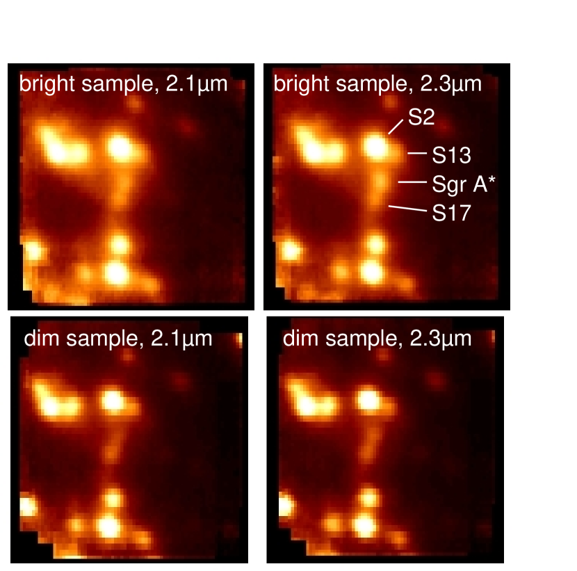
Figure 1.— The Galactic Center as seen with SINFONI. Channel maps from the bright and the dim sample obtained by taking the mean in spectral dimension from $2.05\,\mu$m to $2.15\,\mu$m and from $2.25\,\mu$m to $2.35\,\mu$m. All images are scaled the same way and use an identical color map. Sgr A* is brighter in the longer wavelength maps, indicating that it is is redder than the field stars. Furthermore, the effect is more pronounced in the dim sample, meaning that Sgr A* is redder therein than in the bright sample.

The reduction of the SINFONI data followed the standard steps: From all source data we subtracted the respective sky frames to correct for instrumental and atmospheric background. We applied flatfielding, bad pixel correction, a search for cosmic ray hits, and a correction for the optical distortions of SINFONI. We calibrated the wavelength dimension with line emission lamps and tuned on the atmospheric OH-lines of the raw frames. Finally we assembled the data into cubes with a spatial grid of 12.5 mas/pix.

3. Analysis

Figure 2.— Lightcurve and variation of the spectral power law index $\beta$ during the flare. Time is counted from 2:40 UT. Top: Flux ratio flare/S2. Thin dots are exposures affected by bad seeing. Middle/top: $\beta$ using the small apertures background. Middle/bottom: $\beta$ using the off state subtraction background. Bottom: $\beta$ using the constant subtraction background.

3.1. Flux determination

For all 44 cubes we extracted a collapsed image (median in spectral dimension) of a rectangular region (0.25”$\times$0.5”) centered on Sgr A* and containing the three S-stars S2, S13, and S17. We determined the flux of Sgr A* from a fit with five Gaussians to each of these images. Four Gaussians with a common width describe the four sources. The fifth Gaussian (with a width $3.5\times$ wider, typical for the halo from the imperfect AO correction) accounts for the halo of the brightest star S2 ($K\approx 14\,$mag). The halos of the weaker sources (all $K<15\,$mag) could be neglected for the flux measurement. We fixed the positions of all sources (known a-priori from a combined cube) and the amplitude ratios for the stars. Five parameters were left free: An overall amplitude, the background, the width, the flux ratio halo/S2, and $\cal{F}$, the flux ratio Sgr A*/S2. This procedure disentangles real variability from variations in the background, the Strehl ratio, and the seeing.

As a crosscheck we determined $\cal{F}$ in a second way for all images; for both Sgr A* and S2 we measured the flux difference between a signal region centered on source and a reasonable, symmetric background region. The such determined values agreed very well with the fits. For further analysis we used the fitted ratios and included the difference between the two estimates in the errors.

3.2. Choice of background

The value of the spectral power law index $\beta$ crucially depends on the background subtraction. Subtracting too much light would artificially make the signal look redder than it is. Hence, a reasonable choice for the background region excludes the nearby sources S2 and S17. Furthermore, the background flux is varying spatially. Actually Sgr A* lies close to a saddle point in the background light distribution, caused by S2 and S17 (see Fig. 1). In the East-West direction the background has a maximum close to Sgr A* and in the North-South direction a minimum. A proper estimate of the background can be achieved in two ways: a) working with small enough, symmetric apertures, and b) subtracting from the signal an off state obtained at the position of Sgr A* from cubes in which no emission is seen. We used the first method as well as two variants of the second.
Small apertures: The local background at a position $\vec{x}$ can be estimated by averaging over a small, symmetric region centered on $\vec{x}$. Given the background geometry we have chosen a ring with inner radius $3\,$pix and outer radius $7\,$pix. The circular symmetry was only broken since we explicitely excluded those pixels with a distance to S17 and S2 smaller than 3 and 7 pixels respectively. Unfavorable of this method is that the local background is only approximated, since a sufficiently large region has to be declared as signal region.
Off state subtraction: The local background can be extracted from cubes in which no signal is seen. Since the seeing conditions change from cube to cube, one still has to correct for the varying amount of stray light in the signal region. We estimate this variation by measuring the difference spectrum between signal and off cube in a stray light region. The latter must not contain any field stars and should be as far away from the nearby sources as Sgr A*. We used two stray light regions to the left and to the right of Sgr A*, between 5 and 10 pixels away. The disadvantage of this method is that one needs a suitable off state. The latter point is critical for our data. Even though Sgr A* has not been detected directly in the first three cubes, the light at its position appears redder than the local background. Assuming that this light is due to a very dim, red state of Sgr A*, we would subtract too much red light and artificially make the flare too blue. In this sense, this method yields an upper limit for $\beta$.
Constant subtraction: The off state method can be varied to obtain a lower limit for $\beta$. Assuming that the true off state spectrum has the color of S2, one can demand that it is flat after division by S2. In our data, the S2 divided off state spectrum is rising towards longer wavelengths. Hence, in this third method we estimate the background at blue wavelengths and use that constant as background for all spectral bins.

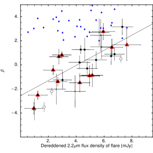
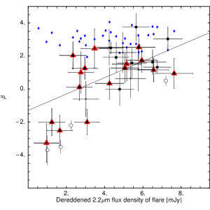
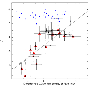
Figure 3.— Correlation plots between the flare flux and the spectral index $\beta$. Points with error bars represent the flare, blue dots are $\beta_{S17}$. Thick black dots mark the points with an error $\Delta\beta<1$, red triangles mark the data with good seeing (FWHM $<75\,$ mas). The line is a fit to the thick black dots. Open circles denote the data from Eisenhauer et al. (2005) - near 2 mJy - and Ghez et al. (2005b) - near 7 mJy. Left: Small apertures method; middle: off state subtraction method; right: constant subtraction method.

3.3. Determination of spectral power law index

We obtained spectra as the median of all pixels inside a disk with radius $3\,$pix centered on source minus the median spectrum of the pixels in the selected off region. In order to correct for the interstellar extinction we then divided by the S2-spectrum (obtained in the same way as the signal). Next the temperature of S2 is corrected by multiplying by the value of $\nu S_{\nu}$ of a blackbody with $T\approx 25000\,$K. After binning the data into 60 spectral channels it is finally fit with a power law $\sim\nu^{\beta}$. With this definition, red emission has $\beta<0$. The error on $\beta$ is obtained as the square sum of the formal fit error and the standard deviation in a sample of 20 estimates for $\beta$ obtained by varying the on and off region selection.

4. Results

We observed a strong (flux density up to $8\,$mJy or $\nu L_{\nu}\approx 10^{35}\,$ergs/s), long (more than 3 hours) flare which showed significant brightness variations on timescales as short as 10 minutes (Fig. 2, top). While the data is not optimal for a periodicity search (poorer sampling than our previous imaging data), it is worth noting that the highest peak in the periodogram (significance of $\approx 2\,\sigma$) lies at a period of $\approx 18\,$min. This is also the timescale found by Genzel et al. (2003), who identify the quasi-periodicity with the orbital time close to the last stable orbit (LSO) of the MBH.

We divided the data into three groups: a) the cubes of the first peak near $t=50\,$min (”preflare”), b) the cubes at $t>100\,$min with $\cal{F}\,$$<$ 0.25 (”dim state”), and c) the cubes at $t>100\,$min with $\cal{F}\,$$>$ 0.25 (”bright state”). For the three sets we created combined cubes in which we determined $\beta$, using all three background estimates. In all cases we obtained the correct spectral index $2.9\pm 0.5$ for S17 (a star with a spectrum similar to S2 but a flux comparable to Sgr A*). For Sgr A* we get:

$\beta\,\,$	preflare	dim state	bright state
off state subtr.	$-1.4\pm 0.4$	$-0.7\pm 0.4$	$+0.4\pm 0.2$
small apertures	$-1.8\pm 0.3$	$-1.7\pm 0.4$	$-0.1\pm 0.3$
constant subtr.	$-3.4\pm 0.4$	$-2.3\pm 0.3$	$-0.3\pm 0.2$

The values obtained from the small apertures lie between the values from the other two methods, consistent with the idea that they yield upper and lower limits. The absolute values vary systematically according to the chosen background method. However, independent from that, it is clear that the preflare is redder than the dim state which in turn is redder than the bright state. An obvious question then is whether flux and $\beta$ are directly correlated.

Hence, we applied the spectral analysis to the individual cubes. We kept the data in which Sgr A* is detected, the error $\Delta\beta<1.5$ and the spectral index for S17 does not deviate more than $1.5$ from the expected value. The resulting spectral indices appear to be correlated with the flux (Fig. 2, 3). The values match the results in Eisenhauer et al. (2005) and Ghez et al. (2005b). Bright flares are indeed bluer than weak flares, as suspected by Ghez et al. (2005b) and consistent with the earlier multi-band observations of Genzel et al. (2003). Our key new result is that this even holds within a single event.

For all three background methods it is clear that the main event was preceded by a weak, red event. For the small apertures and the constant subtraction method instantaneous flux and spectral index are correlated. For the off state subtraction method one could instead group the data into a preflare at the beginning and a bluer, brighter main event.

We checked our data for contamination effects. If stray light would affect the flare signal, $\beta$ should be correlated with the seeing (measured by the width from the multiple fits). Since we did not find such a correlation, we exclude significant contamination.

5. Interpretation

Theoretical models predict that the mm-IR emission from Sgr A* is synchrotron emission from relativistic electrons close to the LSO (Liu & Melia, 2001; Quataert, 2003; Liu et al., 2004, 2006). Radiatively inefficient accretion flow (RIAF) models with a thermal electron population ($T_{\mathrm{e}}\approx 10^{11}\,$K) produce the observed peak in the submm but fail to produce enough flux at 2$\,\mu$m. The NIR emission requires transiently heated or accelerated electrons as proposed by Markoff et al. (2001).

A conservative interpretation of our data is suggested by Fig. 3, middle. There was a weak, red event before and possibly independent from the main flare which was a much bluer event. Plausibly the preflare is then due to the high-energetic tail of the submm peak (Genzel et al., 2003). The main flare requires nevertheless a population of heated electrons.

A more progressive interpretation follows from the correlation between flux and $\beta$ (Fig. 3, left & right). It suggests that the NIR variability is caused by the combination of transient heating with subsequent cooling and orbital dynamics of relativistic electrons. In the following subsections we will exploit this idea.

5.1. Synchrotron emission

In the absence of continued energy injection, synchrotron cooling will suppress the high energy part of the electron distribution function. This results in a strong cutoff in the NIR spectrum with a cutoff frequency decreasing with time. At a fixed band one expects that the light becomes redder as the flux decreases. This can cause the correlation between flux and $\beta$. The observed flare apparently needs several heating and cooling events.

The synchrotron cooling time is comparable to the observed timescale of decaying flanks as in Fig. 2 (top) or Genzel et al. (2003). In a RIAF model (Yuan et al., 2003) the magnetic field $B$ is related to the accretion rate $\dot{M}$. For disk models with $\dot{M}\approx 10^{-8}\,M_{\odot}/$yr (Agol, 2000; Quataert & Gruzinov, 2000) one has $B\approx 30\,$G at a radial distance of $3.5\,R_{\mathrm{S}}$ (Schwarzschild radii). The cooling time for electrons emitting at $\lambda=2\,\lambda_{2}\,\mu$m for $B=30\,B_{30}\,$G is

$$t_{\rm cool}\approx 8\,B_{30}^{-3/2}\,\lambda_{2}^{1/2}\,{\rm min}\,\,.$$ (1)

This is similar to the orbital timescale, making it difficult to disentangle flux variations due to heating and cooling from dynamical effects due to the orbital motion.

5.2. Orbital dynamics

The timescale of $\approx 20$ minutes for the observed variations suggests orbital motion close to the LSO as one possible cause. Any radiation produced propagates through strongly curved space-time. Beaming, multiple images, and Doppler shifts have to be considered (Hollywood et al., 1997, 1999). Recent progress has been made in simulating these effects when observing a spatially limited emission region orbiting the MBH (Paumard et al., 2005; Broderick & Loeb, 2005a, b, c).

That the emission region is small compared to the accretion disk can be deduced from X-ray observations. Eckart et al. (2004, 2005) report similar timescales for X-ray- and IR-flares. This excludes that the X-ray emission is synchrotron light as one would expect cooling times $<1\,$min (eq. 1). The X-ray emission is naturally explained by IC scattering of the transiently heated electrons that have a $\gamma$-factor of $\gamma\approx 10^{3}$. The IC process scatters the seed photon field up according to $\nu_{\mathrm{IC}}\approx\gamma^{2}\,\nu_{\mathrm{seed}}$. Given $\nu_{\mathrm{IC}}\approx 10^{18}\,$Hz for X-rays the seed photon frequency is $\nu_{\mathrm{seed}}\approx 10^{12}\,$Hz - the submm regime. The X-ray intensity for the synchrotron-self-Compton case is given by

$$X/IR=L_{\mathrm{SSC}}/L_{\mathrm{sync}}\approx 10^{-2}L_{35}\left(R/R_{\mathrm{S}}\right)^{-2}B_{30}^{-2}\,\,,$$ (2)

where $L_{35}$ is the seed photon field luminosity in units of $10^{35}\,$ergs/s and $R$ the radius of the emission region. The highest value of $L_{35}$ compatible with the MIR- and submm-data is reached for a flat spectrum ($\beta=0$) of the heated electrons. Thus, $L_{35}\lesssim 1$. Via equation (2) we have $R/R_{\mathrm{S}}\approx 0.1\sqrt{L_{35}/(X/IR)}$. From the observed ratios $X/IR\approx[0.1\,-\,1]$ we derive $R<0.3\,R_{\mathrm{S}}$. That means, the emission region has to be a small spot.

A plausible dynamical model is discussed in Paumard et al. (in prep). It reproduces typical lightcurves as observed by Genzel et al. (2003) or in Fig. 2. Due to the Doppler effect the observed light corresponds to different rest frame frequencies depending on the orbital phase. If the source spectrum is curved, flux and spectral index appear correlated. Following this interpretation, the emission during the brightest part originates from a rest-frequency with larger $\beta$ than the dimmer state emitted at shorter wavelengths. Such a concavely curved spectrum is naturally expected from the synchrotron models.

References

- Agol (2000) Agol, E. 2000, ApJ, 538, L121
- Bonnet et al. (2004) Bonnet, H. et al. 2004, ESO Messenger, 117, 17
- Broderick & Loeb (2005a) Broderick, A. & Loeb, A. 2005, MNRAS, 363, 353
- Broderick & Loeb (2005b) Broderick, A. & Loeb, A., ApJ, 636, L109
- Broderick & Loeb (2005c) Broderick, A. & Loeb, A., MNRAS, submitted (astro-ph/0509237)
- Eckart et al. (2004) Eckart, A. et al. 2004, A&A, 427, 1
- Eckart et al. (2005) Eckart, A. et al., A&A, in press (astro-ph/0512440)
- Eisenhauer et al. (2003) Eisenhauer, F. et al. 2003, Proc. SPIE, 4841, 1548
- Eisenhauer et al. (2005) Eisenhauer, F. et al. 2005, ApJ, 628, 246
- Genzel et al. (2003) Genzel, R. et al. 2003, Nature, 425, 934
- Ghez et al. (2003) Ghez, A. et al. 2003, ApJ, 586, L127
- Ghez et al. (2004) Ghez, A. et al. 2004, ApJ, 601, L159
- Ghez et al. (2005a) Ghez, A., Salim, S., Hornstein, S., Tanner, A., Lu, J., Morris, M. & Becklin, E. 2005, ApJ, 620, 744
- Ghez et al. (2005b) Ghez, A. et al. 2005, ApJ, 635, in press
- Hollywood et al. (1997) Hollywood, J. & Melia, F. 1997, ApJS, 112, 423
- Hollywood et al. (1999) Hollywood, J., Melia, F., Close, L., McCarthy, D., Dekeyser, T. 1999, ApJ, 448,
- Liu & Melia (2001) Liu, S. & Melia, F. 2001, ApJ, 561, L77
- Liu et al. (2004) Liu, S., Petrosian, V. & Melia, F. 2004, ApJ, 611, L101
- Liu et al. (2006) Liu, S., Melia, F. & Petrosian, V. 2006, ApJ, 636, L798
- Markoff et al. (2001) Markoff, S., Falcke, H., Yuan, F. & Biermann, P. 2001, A&A, 379, L13
- Melia et al. (2000) Melia, F., Liu, S. & Coker, R. 2000, ApJ, 545, L117
- Melia et al. (2001) Melia, F., Liu, S. & Coker, R. 2001, ApJ, 553, 146
- Narayan et al. (1995) Narayan, R., Yi, I., & Mahadevan, R. 1995, Nature, 374, 623
- Paumard et al. (2005) Paumard, T. et al. 2005, AN, 326, 568
- Quataert & Narayan (1999) Quataert, E. & Narayan, R. 1999, ApJ, 520, 298
- Quataert & Gruzinov (2000) Quataert, E. & Gruzinov, A. 2000, ApJ, 539, 809
- Quataert (2003) Quataert, E. 2003, ANS, 324, 435
- Schödel et al. (2002) Schödel, R. et al. 2002, Nature, 419, 694
- Yuan et al. (2003) Yuan, F., Quataert, E. & Narayan, R. 2003 ApJ, 598, 301