About putative Neptune-like extrasolar planetary candidates

Abstract

Context. We re-analyze the precision radial velocity (RV) data of HD 208487, HD 190360, HD 188015 and HD 114729. These stars are supposed to host Jovian companions in long-period orbits.

Aims. We test a hypothesis that the residuals of the 1-planet model of the RV or an irregular scatter of the measurements about the synthetic RV curve may be explained by the existence of additional planets in short-period orbits.

Methods. We perform a global search for the best fits in the orbital parameters space with genetic algorithms and simplex method. This makes it possible to verify and extend the results obtained with an application of commonly used FFT-based periodogram analysis for identifying the leading periods.

Results. Our analysis confirms the presence of a periodic component in the RV of HD 190360 which may correspond to a hot-Neptune planet. We found four new cases when the 2-planet model yields significantly better fits to the RV data than the best 1-planet solutions. If the periodic variability of the residuals of single-planet fits has indeed a planetary origin then hot-Neptune planets may exist in these extrasolar systems. We estimate their orbital periods in the range of 7–20 d and minimal masses about of 20 masses od the Earth.

1 Introduction

The precision radial velocity (RV) surveys for extrasolar planets approach the limit of detection of Neptune-like companions. In the past year, 14-Earth mass planet has been announced by Santos et al. (2004). A low-mass companion has been found in the ${\rho}^{1}$ Cancri system (McArthur et al., 2004). Almost at the same time, a Neptune-like planet has been also discovered by Butler et al. (2004). Very recently, Rivera et al. (2005) announced a discovery of $\sim 7$ Earth-mass planet in $\sim 2$d orbit about the famous Gliese 876 planetary system. Also Vogt et al. (2005) announced a new multi-planet system about HD 190360 involving a Neptune-mass planet in $\simeq 17.1$d orbit with a Jupiter-like companion with $\sim 3000$d orbital period. These discoveries change the view of multi-planet systems. The found low-mass planets likely are rocky bodies rather than massive gaseous hot-Jupiters. The architecture of their environment, involving also giant planets in relatively distant orbits, begin to resemble our own Solar system.

There are already speculations as to which of the extrasolar systems involving Jupiter-like planets can contain smaller companions. At present, such objects cannot be clearly detected because of small amplitude of the contributed RV signal and not frequent enough observations. Nevertheless, the existence of such planets seems to be natural. The dynamical relaxation of planetary systems (Adams & Laughlin, 2003) can lead to final configurations with orbits filling up the dynamically available space of stable orbits (Laskar, 2000). In particular, many extrasolar systems containing distant Jupiter-like planets may contain smaller, still undetectable companions, which can easily survive in a close neighborhood of the parent star. Baraffe et al. (2005) show that the three recently detected hot-Neptune planets (about GJ 436, $\rho^{1}$ Cnc, $\mu$ Arae) may originate from more massive gas giants which have undergone significant evaporation. This work suggests that hot-Neptunes and hot-Jupiters may share the same origin and evolution history and they can be as frequent as are hot-Jupiters. The numerical simulations by Brunini & Cionco (2005) show that the formation of compact systems of Neptune-like planets close to solar type stars could be a common by-product of planetary accretion. In turn, these theoretical works are supported by several new detections of hot-Neptune and hot-Saturn candidates (e.g., Bonfils et al., 2005; Udry et al., 2005; Curto et al., 2005; Fischer et al., 2005).

The detection of Neptune-mass exoplanets is a breakthrough in the field but the inevitable problem still lies in the limitations of the Doppler technique. The radial velocity signal of small, Neptune-like planets revolving close to the host star has the semi-amplitude of a few meters per second, i.e., at a similar range as the measurement errors and chromospheric variability of the RV. This can be a source of erroneous interpretation of the observations. For instance, in a recent work, Wisdom (2005) claims that the orbital period of 2.38d of companion d detected by McArthur et al. (2004) in ${\rho}^{1}$ Cancri system is an alias of two periods originating from the orbital motion of planets b and c and, instead, he found an evidence of an another planet in $\sim 261$ d orbit. Actually, a proper interpretation of the observations is still very difficult. Often, they can be equally well modeled by qualitatively different configurations and even the number of planets cannot be resolved without doubt. An example will be given in this paper too.

In this work, for a reference and a test of our approach, we re-analyze the published RV data of two stars: HD 208487 (Tinney et al., 2005)— Gregory (2005a) claims that a second planet accompanies a confirmed Jovian companion b, and HD 190360 (Vogt et al., 2005)—the discovery team claims the existence of a hot-Neptune and a Jovian planet in long-period orbit. Next, using the same method, we study other three extrasolar systems: HD 188015 (Marcy et al., 2005b), HD 114729 (Butler et al., 2003) and HD 147513 (Mayor et al., 2004), in which Jupiter-like companions have been discovered in long-period orbits. However, the residuals of the 1-Keplerian fits are either relatively large or we see ”suspicious” scatter of the residuals. We use the available measurements to test a hypothesis that additional short-period planets exist in these systems and their signals may be already hidden in the existing data, but likely at the detection limit. Our reasoning follows the theoretical predictions that Neptune-like planets can easily form and survive close to the parent star. The main difficulty is a small number of measurements, typically about of 30–40 data points spread over several years. It makes it very difficult to determine orbits of such planetary candidates without a doubt. In particular, this concerns the identification of the orbital periods with the application of somehow traditional Fourier-based analysis. Instead, we prefer a global search for the best-fit 2-planet configurations using the genetic algorithms and scanning ${(\chi^{2}_{\nu})^{1/2}}$ in the multidimensional space of orbital parameters. This could be an alternative to the already classic Lomb-Scargle periodogram (e.g., Butler et al., 2004) or sophisticated Bayesian-based analysis, which is recently proposed by Gregory (2005a, b). That author claims an evidence of additional planets using the same RV measurements which are modeled by 1-planet configurations by the discovery teams, about HD 73526 and HD 208487.

2 The fitting algorithm, numerical setup and tests

In all cases studied in this paper, we assume that the second, putative planet is closer to the star than the already known companion b in relatively long-period orbit. To model the RV signal, we use the standard formulae (e.g., Smart, 1949). For every planet, the contribution to the reflex motion of the star at time $t$ is the following:

$$V_{{\mbox{\scriptsize r}}}(t)=K[\cos(\omega+\nu(t))+e\cos\omega]+V_{0},$$ (1)

where $K$ is the semi-amplitude, $\omega$ is the argument of pericenter, $\nu(t)$ is the true anomaly involving implicit dependence on the orbital period $P$ and the time of periastron passage $T_{{\mbox{\scriptsize p}}}$, $e$ is the eccentricity, $V_{0}$ is the velocity offset. There are some arguments that is best to interpret the derived fit parameters $(K,P,e,\omega,T_{{\mbox{\scriptsize p}}})$ in terms of Keplerian elements and minimal masses related to Jacobi coordinates (Lee & Peale, 2003; Goździewski et al., 2003).

To search for the best-fit solutions, we applied a kind of hybrid optimization. A single program run starts the genetic algorithms (GAs) optimization. In particular, we use the PIKAIA code by Charbonneau (1995). The GAs has many advantages over more popular gradient-type algorithms, for instance, the Levenberg-Marquardt scheme (Press et al., 1992). The power of GAs lies in their global nature, the requirement of knowing only the ${(\chi^{2}_{\nu})^{1/2}}$ function and an ease of constrained optimization. In particular, GAs permit to define parameter bounds or add a penalty term to ${(\chi^{2}_{\nu})^{1/2}}$ (Goździewski et al., 2003, 2005).

In our code, the initial population of randomly chosen 2048 members represents potential solutions to the RV model. The code produce 128 new off-spring generations. The best fit found by PIKAIA is refined by the simplex algorithm of Melder and Nead (Press et al., 1992). In that method, we set the fractional tolerance for ${(\chi^{2}_{\nu})^{1/2}}$ variability to $10^{-15}$. Such procedure runs thousands of times for every analyzed data set. Thanks to non-gradient character of both algorithms we may bound the space of examined parameters, according to specific requirements. Usually, due to a small number of measurements, the best-fit $e_{{\mbox{\scriptsize c}}}$ is barely constrained and tends to be large, in particular in the range of very short periods. Nevertheless, we assumed that the tidal circularization limits the eccentricity of the short-period orbit and we arbitrarily set its upper bound to 0.3. The orbital periods of putative planets are searched in the range of [2,136] d.

The internal errors of the RV data are rescaled according to $\sigma^{2}=\sigma_{{\mbox{\scriptsize m}}}^{2}+\sigma_{{\mbox{\scriptsize j}}}^{2},$ where $\sigma$ is the joint uncertainty, $\sigma_{{\mbox{\scriptsize m}}}$ and $\sigma_{{\mbox{\scriptsize j}}}$ is the internal error and adopted variance of stellar jitter, respectively. Typically, we choose $\sigma_{{\mbox{\scriptsize j}}}$ following estimates for Sun-like dwarfs (Wright, 2005) or we set its value as quoted by the discovery teams. The particular estimates are given in Table 1.

The best fits found in the entire hybrid search are illustrated by projections onto planes of particular parameters of the RV model, Eq. 1. Usually, we choose the $(P,K)$- and $(P,e)$-planes. Marking the elements within the formal $1\sigma,2\sigma,3\sigma$ confidence intervals of the best-fit solution (which is always marked in the maps by two crossing lines) we have a convenient way of visualizing the shape of the local minima of ${(\chi^{2}_{\nu})^{1/2}}$ and to obtain reasonable estimates of the fit errors (Bevington & Robinson, 2003).

Still, even we find very good best-fit configurations, a problem persists: is the obtained fit not an artifact caused by specific time-distribution of measurements or the stellar jitter? In order to answer for this question we apply the test of scrambled velocities (Butler et al., 2004). We remove the synthetic RV contribution of the firstly confirmed planet from the RV data, according to its best-fit parameters. Next, the residuals are randomly scrambled, keeping the exact moments of observations, and we search for the best-fit elements of the second (usually, inner) planet. For uncorrelated residual signal we should get close to the Gaussian distribution of ${(\chi^{2}_{\nu})^{1/2}}$. For every synthetic data set, the minimization is performed with the hybrid method. Let us note, that in this case we deal with 1-planet model (and 6 parameters only) thus the large population in the GA step and precise simplex code assure that the best-fit solution can be reliably found in one single run of the hybrid code. The runs of the code are repeated at least 20,000 times for every analyzed data set. If the best fit corresponding to the real (not scrambled) data lies on the edge of this distribution, such experiment assure us that the real data produce much smaller ${(\chi^{2}_{\nu})^{1/2}}$ (and an rms) than the most frequent outcomes obtained for the scrambled data. Such a test provides a reliable indication that the residuals are not randomly distributed. A likelihood $p_{{\mbox{\scriptsize H}}}$ that the residuals are only a white noise can be measured by the ratio of the best fits with ${(\chi^{2}_{\nu})^{1/2}}$ less or equal to that one corresponding to the real data against all possible solutions.

Unfortunately, even with a positive outcome of the test of scrambled residuals we still are not done. Even if we find a strong indication that the residuals are not randomly distributed, and we find a periodic component in the residual signal, then we still cannot be sure that it has a planetary origin and it does not eliminate jitter as a source of the RV signal. We are warned by the referee (and here we literally follow his arguments) that jitter can have some spectral power usually associated with the rotation period of the star, but other peaks can be present. The spectral structure of very low-amplitude jitter is not well-known yet, but for large amplitude jitter in active star, the power spectrum can show several peaks and aliases. One example is HD 128311 in Butler et al. (2003); an another one is, possibly, HD 147513 (Mayor et al., 2004) analyzed in this work. Therefore, the noisy periodic signal may be due to jitter and it may be possible that some secondary periods, which are present in the residual signals, are corresponding to aliases of the stellar rotation period reinforced by the noise. This is the main reason why our work cannot be considered in terms of a discovery paper; additional measurements and analysis are required to confirm (or withdraw) the hypothesis about the planetary nature of the RV variability. Our basic goal is to test the approach on a few non-trivial and, possibly, representative examples. We try to find characteristics of the RV data sets which can confirm the periodogram-based approach (e.g., Butler et al., 2004) and, possibly, may be helpful to extend its results. Our analysis may be useful to speed-up the detections of new planets and planning the strategy of future observations.

2.1 Test case I: HD 208487

The first test case of HD 208487 (Tinney et al., 2005) illustrates nuances of modeling the RV data. The observational window of this star spans about of 2500 d but the number of data points is only 31. The discovery team found a planetary companion with minimal mass of 0.7 $m_{{\mbox{\scriptsize J}}}$ and orbital period about of 130 d. An rms of this 1-planet solution is $\sim 7$ m/s, while the joint uncertainty is about of $6$ m/s, assuming jitter estimate of 3 m/s, a reasonable value for the quiet, 6 Gyr old star with $R_{HK}^{\prime}\simeq-4.90$ (Tinney et al., 2005). The data have been reanalyzed by Gregory (2005a). He applied his Bayes-periodogram method and found much better 2-planet solution, explaining the residual signal of the 1-planet solution by the presence of a distant, second companion in 998 d orbit. This solution has significantly better rms of 4.2 m/s and ${(\chi^{2}_{\nu})^{1/2}}\simeq 0.83$ than the best single planet solution, ${(\chi^{2}_{\nu})^{1/2}}=1.27$.

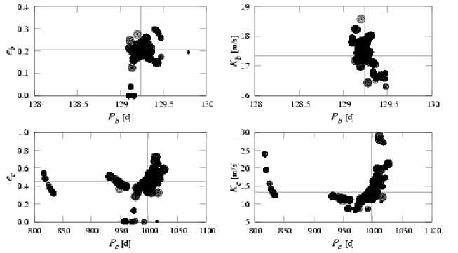
Figure 1: The parameters of the best-fit solutions to the 2-planet model of the HD 208487 RV data projected onto the ($P,e$)- and ($P,K$)-plane. In this search, a more distant companion to the formerly known Jupiter-like body in $\simeq 130$ d orbit is assumed. Upper plots are for the inner planet, bottom plots are for the outer companion. The values of ${(\chi^{2}_{\nu})^{1/2}}$ of the best-fit solutions are marked by the size of symbols. Largest circle is for ${(\chi^{2}_{\nu})^{1/2}}$ equal to 0.619 ; smaller symbols are for 1$\sigma$ solutions with ${(\chi^{2}_{\nu})^{1/2}}\in[0.619,0.710)$, 2$\sigma$ solutions with ${(\chi^{2}_{\nu})^{1/2}}\in[0.710,0.841)$ and 3$\sigma$ solutions with ${(\chi^{2}_{\nu})^{1/2}}\in[0.841,1.0)$ (smallest, filled circles), respectively.

The analysis of the HD 208487 data is a good reference for our simpler approach. First we did the hybrid search for the best 2-planet configurations, assuming that 130 d $<P_{{\mbox{\scriptsize c}}}<$ 1200 d. The results of this search are illustrated in Fig. 1. Curiously, the best-fit has ${(\chi^{2}_{\nu})^{1/2}}\simeq 0.62$ and an rms $\simeq 3.1$ m/s, so it is apparently better than the fit quoted by Gregory (2005a). The best-fit parameters $(K,P,e,\omega,T_{{\mbox{\scriptsize p}}}-T_{0})$ are: $(17.532\leavevmode\nobreak\ \mbox{m/s},129.224\leavevmode\nobreak\ \mbox{d},0.195,188^{\circ}.232,1421.112\leavevmode\nobreak\ \mbox{d})$ and $(13.117\leavevmode\nobreak\ \mbox{m/s},997.953\leavevmode\nobreak\ \mbox{d},0.433,190^{\circ}.470,2358.258\leavevmode\nobreak\ \mbox{d})$ for the inner and outer planet, respectively (where $T_{0}$=JD 2,450,000) and $V_{0}=9.64$ m/s. Note much larger eccentricity of the outer planet than in the fit by Gregory (2005a), $e_{{\mbox{\scriptsize c}}}\simeq 0.2$. The $1\sigma$ scatter of the derived solutions around the best-fit (Fig. 1) provides the error estimate of the orbital elements. In general, the parameters of the inner planet are well fixed, while the elements of the outer body have much larger formal uncertainties. The errors of $K_{{\mbox{\scriptsize c}}},P_{{\mbox{\scriptsize c}}},e_{{\mbox{\scriptsize c}}}$ are about of 100 d, 0.3, and $10$ m/s, respectively.

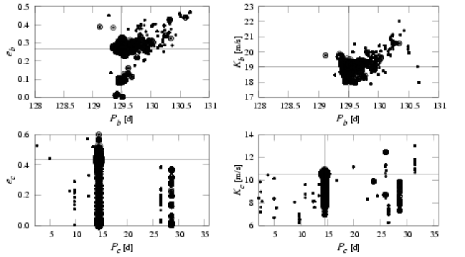
Figure 2: The parameters of the best-fit solutions to the 2-planet model of the HD 208487 RV data projected onto ($P,e$)- and ($P,K$)-plane. In this search, an inner companion to the formerly known Jovian planet in $\simeq 130$ d orbit is assumed. Upper plots are for the outer planet, bottom plots are for the inner companion. The values of ${(\chi^{2}_{\nu})^{1/2}}$ of the best-fit solutions are marked by the size of symbols. Largest circle is for ${(\chi^{2}_{\nu})^{1/2}}=0.581$ (the best-fit solution, Table 1); smaller symbols are for solutions within $1\sigma$ interval of the best-fit with ${(\chi^{2}_{\nu})^{1/2}}\in[0.581,0.677)$, 2$\sigma$ solutions with ${(\chi^{2}_{\nu})^{1/2}}\in[0.677,0.813)$ and 3$\sigma$ solutions with ${(\chi^{2}_{\nu})^{1/2}}\in[0.813,0.98)$ (smallest, filled circles), respectively.

Figure 3: Stability analysis of the orbital fit with putative Neptune-like body in the HD 208487 system. The upper panel is for the eccentricities, the lower panel is for MEGNO computed for $3\cdot 10^{5}$ orbital periods of the outer companion.

Next, we explored the inner space to the $\sim 130$ d orbit, assuming 2 d $<P_{{\mbox{\scriptsize c}}}<$ 130 d. Surprisingly, we found ever better fit, given in Table 1, with ${(\chi^{2}_{\nu})^{1/2}}\simeq 0.581$ and an rms $\simeq 2.82$ m/s. The orbital elements of the best-fit solutions found in the entire search are projected onto the parameter planes and they are illustrated in Fig. 2. Note a small scatter of the elements of the outer planet and two sharp minima in $P_{{\mbox{\scriptsize c}}}$. The best-fit has $P_{{\mbox{\scriptsize c}}}\simeq 14.5$ d and $e_{{\mbox{\scriptsize c}}}\simeq 0.42$. Such large eccentricity may contradict the requirement of a tidally circularized orbit. However, the orbital evolution of the whole system reveals large-amplitude variations of $e_{{\mbox{\scriptsize c}}}$ (Fig. 3) which are forced by the mutual interactions between companions. We also face an another trouble, a small periastron-apoastron distance of the two putative planets $\sim 0.2$ AU. Nevertheless, the system appears to be dynamically stable. The evolution of the MEGNO indicator (Goździewski et al., 2001) computed over $3\cdot 10^{5}P_{{\mbox{\scriptsize b}}}$ is illustrated in the lower panel of Fig. 3. Its oscillations about of 2 mean a quasi-periodic configuration and strictly confirm apparently regular behavior of $e_{{\mbox{\scriptsize b,c}}}$.

Figure 4: Lomb-Scargle periodogram of the residuals of the Jupiter-like companion’s with $P_{{\mbox{\scriptsize b}}}\sim 130$ d about HD 208487.

Figure 5: Synthetic RV signals of the two solutions to the RV data of HD 208487. The thick line is for the outer companion to the known $130$ d planet. The thin line is for the putative inner companion. The original RV data are marked with error-bars. For a clear illustration, only a part of the second curve is plotted.

For a reference, we computed the Lomb-Scargle (LS) periodogram (Fig. 4) of the residuals of the dominant 1-planet signal having the period of $130$ d. The largest peaks about of 28 d and 998 d (the period of a hypothetic long-period planet) most possibly are aliasing with the best-fit period $\simeq 14.5$ d. However, this period is favored by the smallest ${(\chi^{2}_{\nu})^{1/2}}$. The aliasing of the two dominant periods is illustrated in Fig. 5. This figure shows the synthetic RV signals of the putative configurations with the short- and long-period companions of planet b. Curiously, the orbital periods of the two planets in the model with the short-period orbit are very close to the 9:1 ratio. This again could be an effect of aliasing, nevertheless the best-fit solution with single planet has $P_{{\mbox{\scriptsize b}}}$ about of $14.5$ d and much larger rms $\sim 7$ m/s than in the best 2-planet solution.

Some more interesting results brings the test of scrambled residuals, Fig. 6. It appears that the real residual signal lies far from the maximum of the Gaussian-like distribution and it is unlikely that the residuals are only a white noise ($p_{{\mbox{\scriptsize H}}}\simeq 3\cdot 10^{-5}$). Also $K_{{\mbox{\scriptsize b}}}\simeq 10.5$ m/s is much larger than the joint uncertainty of the measurements. Because HD 208487 is a very old and quiet G-dwarf with low chromospheric activity (Tinney et al., 2005), the hypothesis of a hot sub-Neptune planet in this extrasolar system seems to be very appealing. A peculiarity of this system could be the proximity to the 9:1 mean motion resonance of its companions.

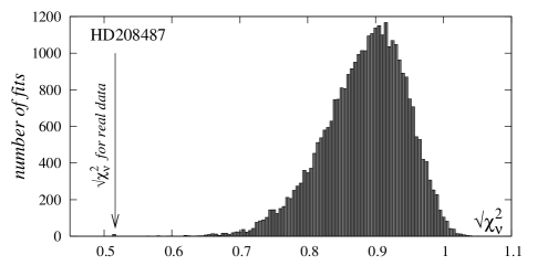
Figure 6: A histogram of ${(\chi^{2}_{\nu})^{1/2}}$ for Keplerian fits to 33,000 sets of scrambled RV residuals of the synthetic signal of the Jupiter-like planet in $\sim 130$ d orbit (HD 208487, see Table 1). The position of the best-fit to the real data is marked with an arrow.

2.2 Test case II: HD 190360

In a recent paper, Vogt et al. (2005) published the precision RV data for HD 190360. The variability of the RV is explained by the existence of two planetary companions: a Jupiter-like planet in long-period orbit, $P_{{\mbox{\scriptsize b}}}\sim 3000$ d, and a Neptune-like body in $\simeq 17.1$ d orbit. The authors conclude that the existence of the smaller planet is the best explanation of the residual signal of the single planet solution. Its contribution has small semi-amplitude $K\simeq 4.6$ m/s. Yet the orbital period is about of a half of the rotational period of the star, 36–44 d, and the RV variability may be an effect of spot complexes on the stellar surface (Vogt et al., 2005).

Figure 7: The parameters of the best-fit solutions to the 2-planet model of the HD 190360 RV data projected onto the ($P,e$)- and ($P,K$)-plane. Upper plots are for the outer planet, bottom plots are for the inner companion. The values of ${(\chi^{2}_{\nu})^{1/2}}$ of the best-fit solutions are marked by the size of symbols. Largest circle is for ${(\chi^{2}_{\nu})^{1/2}}\simeq 0.679$ (the best-fit solution, Table 1); smaller symbols are for 1$\sigma$ solutions with ${(\chi^{2}_{\nu})^{1/2}}\in[0.679,0.70)$, 2$\sigma$ solutions with ${(\chi^{2}_{\nu})^{1/2}}\in[0.70,0.74)$ and 3$\sigma$ solutions with ${(\chi^{2}_{\nu})^{1/2}}\in[0.74,0.79)$ (smallest, filled circles), respectively.

The elements of a few hundred fits gathered by the hybrid search are illustrated in Fig. 7 (the elements of the best-fit are given in Table 1). The period of the inner planet corresponds to a single, very deep minimum of ${(\chi^{2}_{\nu})^{1/2}}$. It is clear, that $e_{{\mbox{\scriptsize c}}}$ has a large error $\sim 0.15$. Our fit is slightly better than that one quoted by Vogt et al. (2005) but $e_{{\mbox{\scriptsize c}}}\simeq 0.2$ is also different as well as we have got slightly larger $K_{{\mbox{\scriptsize c}}}\simeq 5.2$ m/s. Note that we obtain a similar uncertainties of 100 d for $K_{{\mbox{\scriptsize b}}}$ and of 0.05 for $e_{{\mbox{\scriptsize b}}}$.

Figure 8: Lomb-Scargle periodogram of the residuals of the long-period signal which is seen in the HD 190360 data.

The Lomb-Scargle periodogram (Fig. 8) of the residuals of the long-period orbit reveals a strong, dominant peak at $17.1$ d. This an excellent confirmation of the results of the hybrid search. The test of scrambled residuals reveals that the residual signal is hardly random. The maximum of ${(\chi^{2}_{\nu})^{1/2}}$ for scrambled data is shifted by $\simeq 0.4$ from the value of ${(\chi^{2}_{\nu})^{1/2}}$ for the real data.

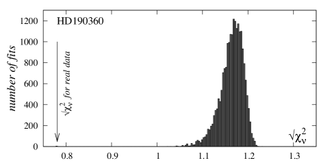
Figure 9: A histogram of ${(\chi^{2}_{\nu})^{1/2}}$ for Keplerian fits to 20,000 sets of scrambled RV residuals of the synthetic signal of the outer planet in HD 190360 (see Table 1). The position of the best-fit to the real data is marked with an arrow.

Now, having so clear picture, we analyze a smaller sample of measurements. To perform this test, we selected 38 first measurements spanning $\sim 2200$ d. The number of data points and their time-coverage are similar to other cases which we study in this work. The described above procedure was repeated on such synthetic data set.

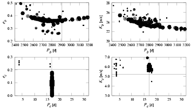
Figure 10: The parameters of the best-fit solutions to the 2-planet model of the RV data of HD 190360 limited to the first 38 measurements, projected onto ($P,e$)- and ($P,K$)-plane. Upper plots are for the outer planet, bottom plots are for the inner companion. The values of ${(\chi^{2}_{\nu})^{1/2}}$ of the best-fit solutions are marked by the size of symbols. Largest circle is for ${(\chi^{2}_{\nu})^{1/2}}\simeq 0.733$; smaller symbols are for 1$\sigma$ solutions with ${(\chi^{2}_{\nu})^{1/2}}\in[0.733,0.793)$, 2$\sigma$ solutions with ${(\chi^{2}_{\nu})^{1/2}}\in[0.793,0.89$ and 3$\sigma$ solutions with ${(\chi^{2}_{\nu})^{1/2}}\in[0.89,1.00)$ (smallest, filled circles), respectively. Vertical and horizontal lines mark the best-fit obtained for the full data (see Fig. 7 and Table 1).

Figure 11: Lomb-Scargle periodogram of the residuals of the long-period signal in HD 190360 when only 38 first measurements are analyzed. Compare with Fig. 8 for the full data set.

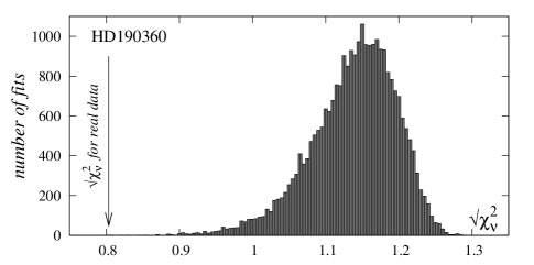
Figure 12: A histogram of ${(\chi^{2}_{\nu})^{1/2}}$ for Keplerian fits to $\sim 27,000$ sets of scrambled RV residuals of the synthetic signal of the outer planet in HD 190360 for the first 38 measurements. The position of the best-fit for the real data is marked with an arrow. Compare with Fig. 9.

Still, the best-fit period of the inner planet can be clearly identified (Fig. 10) but the semi-amplitude $K_{{\mbox{\scriptsize c}}}$ has been slightly shifted. The elements of the outer planet are determined with much larger errors than the uncertainties obtained for the full data. In particular, the error of $P_{{\mbox{\scriptsize b}}}$ is about of 350 d. The dominant period is still well recognizable in the Lomb-Scargle periodogram, Fig. 11. Finally, the test of scrambled residuals also give a clear picture, albeit the histogram (Fig. 12) has much larger width and ${(\chi^{2}_{\nu})^{1/2}}$ of the real data is closer to the maximum of the distribution.

Even for a half of the available measurements, the periodic nature of the residual signal of the single-planet fit can be clearly recognized. One might conclude that the inner planet around HD 190360 might be detected about 2–3 years ago.

The results obtained for the HD 190360 data provide a valuable test of our method and a good reference point to further analysis. Let us recall, that the model with two planets yields low residuals with an rms of $3.5$ m/s and ${(\chi^{2}_{\nu})^{1/2}}$ much smaller than 1, similarly to the three systems which are described below.

3 HD 188015

Recently, Marcy et al. (2005b) published the precision RV of HD 188015. The variability of the RV is explained by the presence of a planetary companion with minimal mass 1.26 $m_{{\mbox{\scriptsize J}}}$ and orbital period $\sim 1.25$ yr. Our attention has been drawn on large rms of this 1-planet solution, $\simeq 8.6$ m/s. The mean error of the RV data is about of 4.1 m/s and expected stellar jitter $\simeq 4$ m/s (Marcy et al., 2005b). The mean measurement error added in quadrature to the jitter is about of 5 m/s, still much smaller than the rms of 1-planet solution. However, this can be partially explained by a linear trend apparently present in the RV signal. If one adds such a trend to the fit model, the rms goes down by 1 m/s (Marcy et al., 2005b, also our Fig. 13a). The trends in the RV data frequently indicate a distant body (e.g., Marcy et al., 2005a; Jones et al., 2002; Goździewski et al., 2003). Nevertheless, we assumed that the second putative body is not a distant companion, but rather a planet closer to the star than already detected companion b.

Figure 13: The best-fit solutions to the RV data published by Marcy et al. (2005b) for HD 188015. a) 1-Kepler model with a linear trend which is apparently present in the data. b) 2-Kepler model is consistent with the measurement error, ${(\chi^{2}_{\nu})^{1/2}}\simeq 1.02$, rms$\simeq 4.9$ m/s. c) Period-phased RV signal of the inner companion. d) A close-up of the synthetic signal of the best-fit 2-planet configuration (see Table 1).

The elements of the best-fit solution found in the entire hybrid search are illustrated in Fig. 13 (panels b,c,d) and its elements are given in Table 1. The synthetic Doppler signal is plotted over the data points in Fig. 13b. Surprisingly, the apparent slope of the RV data can be only an artifact related to a specific time-distribution of measurements. The value of ${(\chi^{2}_{\nu})^{1/2}}\simeq 1.021$ indicates a statistically good solution. Its rms is about of 5 m/s, consistent with the adopted estimate of the mean uncertainty. The semi-amplitude of the inner planets’ signal is $\sim 7$ m/s. Assuming the mass of the host star $\simeq 1.08$ M_☉ (Marcy et al., 2005b), we derived its minimal mass about of 0.07 $m_{{\mbox{\scriptsize J}}}$ and semi-major axis about of 0.08 AU. Thus, the new putative object can be classified as a hot-Neptune planet.

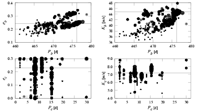
Figure 14: The elements of the best-fit solutions to the 2-planet model of the HD 188015 RV data projected onto the ($P,e$)- and ($P,K$)-plane. Upper plots are for the outer planet, bottom plots are for the inner companion. The ${(\chi^{2}_{\nu})^{1/2}}$ of the best-fit solutions are marked by the size of symbols. Largest circle is for ${(\chi^{2}_{\nu})^{1/2}}=1.021$ (the best-fit solution, Table 1); smaller symbols are for 1$\sigma$ solutions with ${(\chi^{2}_{\nu})^{1/2}}\in[1.02,1.07)$, 2$\sigma$ solutions with ${(\chi^{2}_{\nu})^{1/2}}\in[1.07,1.14)$ and 3$\sigma$ solutions with ${(\chi^{2}_{\nu})^{1/2}}\in[1.14,1.25)$ (smallest, filled circles), respectively.

According to the $1\sigma$-level of ${(\chi^{2}_{\nu})^{1/2}}$, marked in Fig. 14, the uncertainty of $e_{{\mbox{\scriptsize b}}}$ is $\sim 0.1$, and of $K_{{\mbox{\scriptsize b}}}$ is $\sim 5$ m/s. Similarly, the $1\sigma$ uncertainties of the elements of the inner planet can be estimated by $\sim 0.3$ and $1$ m/s, respectively. There are visible several local minima in the $(P_{{\mbox{\scriptsize b}}},e_{{\mbox{\scriptsize b}}})$-plane, which are very narrow with respect to $P_{{\mbox{\scriptsize c}}}$, about of 0.05 d at the $1\sigma$ level. It is clear that the eccentricity of the inner companion (also its argument of periastron — not shown here) cannot be well fixed.

A local minimum at $P_{{\mbox{\scriptsize c}}}\simeq 15.37$ d which also well models the observations (at the $1\sigma$ confidence interval of the best-fit solution) may correspond to an alias of the best-fit period 8.386 d. It could be also an alias of the rotational period $\sim 30$ d of the star, assuming that it is smaller than the 36 d estimate by (Marcy et al., 2005b). Indeed, there is a minimum of ${(\chi^{2}_{\nu})^{1/2}}$ at the $1\sigma$-level of the best-fit about of $30$ d and $e_{{\mbox{\scriptsize c}}}\sim 0.3$, see Fig. 14.

Figure 15: Lomb-Scargle periodogram of the residuals of the long-period signal visible in the RV data of HD 188015.

The results of the hybrid search perfectly agree with the LS periodogram (Fig. 15) of the signal after removal of the contribution from the outer planet. All the relevant periods can be found in the periodogram too. This assures us that the GA search is robust in locating the best-fit solution even in the case when ${(\chi^{2}_{\nu})^{1/2}}$ has several equally deep local minima. Additionally, we did an independent gradient-based scan over $P_{{\mbox{\scriptsize c}}}$ and that test also confirmed the excellent performance of the GAs.

The test of scrambled velocities which is illustrated in Fig. 16 helps us to explain the trouble of finding a clear, secondly dominant short-period in the data. The histogram of ${(\chi^{2}_{\nu})^{1/2}}$ has the maximum about of 1.1 and ${(\chi^{2}_{\nu})^{1/2}}\simeq 0.93$ of the real residuals is not well separated from this maximum. The estimated $p_{{\mbox{\scriptsize H}}}\simeq 0.03$ is significant and indicates that the residual signal is rather noisy. Yet the best 2-planet fit improves significantly the 1-planet solution.

We are warned by the referee (and we quote him again here) that the jitter estimate by Marcy et al. (2005b) comes from the study of jitter levels in the Carnegie planet search sample by Wright (2005). In that article, it turns out that at the activity level of HD 188015 corresponds to an average jitter of the quoted 4 m/s, but with a wide dispersion from case to case, and that levels of 6-7 m/s are not at all uncommon. In fact, for low values of the Calcium index there is little activity-jitter correlation in Wright (2005), and any values between 1 and 10 m/s are almost equally likely. This may invalidate our argument about the excess scatter and the value of ${(\chi^{2}_{\nu})^{1/2}}$ in the 2-planet model. Nevertheless, what we can do is to adopt an uniform jitter variance for all measurements. Then a larger jitter will only ”flatten” ${(\chi^{2}_{\nu})^{1/2}}$, keeping its minimum at similar position in the parameters space. The results for HD 190360 may be used as an argument supporting the planetary hypothesis —in that case the 2-planet fit also has an rms about of 1 m/s smaller than the joint uncertainty. Yet we encountered a similar problem when analyzing the next system, around HD 114729, described below.

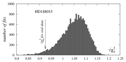
Figure 16: A histogram of ${(\chi^{2}_{\nu})^{1/2}}$ for Keplerian fits to 20,000 sets of scrambled RV residuals of the synthetic signal of the outer planet in HD 188015 (see Table 1). The position of the best-fit to the real data is marked with an arrow.

4 HD 114729

Figure 17: The best-fit solutions to the HD 114729 RV data published in Butler et al. (2003). a) Synthetic signal of 1-planet model. b) 2-Kepler model is consistent with the measurement error, ${(\chi^{2}_{\nu})^{1/2}}\simeq 0.775$, an rms $\simeq 3.6$ m/s. c) Period-phased RV signal of the inner companion. d) A close-up of the synthetic signal of the best-fit 2-planet configuration (see Table 1).

Similarly to most of the stars monitored in precision RV surveys, the HD 114729 is a Sun-like star of G3V spectral type (G0V by Hipparcos). Its RV data indicate a Jupiter-like companion with minimal mass 0.84 $m_{{\mbox{\scriptsize J}}}$, orbital period $\simeq 3.1$ yr and eccentricity $\simeq 0.32$ (Butler et al., 2003). An rms of the single Keplerian fit to the data is 5.34 m/s. It is larger than the mean of internal errors, $\simeq 3.6$ m/s. The expected jitter is 4 m/s (Butler et al., 2003). The mean measurement error scaled in quadrature with the jitter variance is comparable with the rms. Nevertheless, having in mind a significant scatter of the measurements about some parts of the synthetic 1-planet RV curve (see Fig. 17a), and the presence of the distant giant planet, we assumed (as in the previous case) that there exist an another one, inner planet in the system in short-period orbit, [2,136] d. To test this hypothesis, we did the same analysis of the RV data as described in previous sections. The results are illustrated in Fig. 17a,b,c,d which is for the graphical illustration of the best-fit parameters. Figure 18 is for the Lomb-Scargle periodogram of the residual signal of the long-period companion. Figure 19 illustrates the shape of ${(\chi^{2}_{\nu})^{1/2}}$ about the best-fit and the distribution of the best fits obtained in the hybrid search. The orbital parameters of the best fit are given in Table 1. Clearly, the results of the hybrid search agree perfectly with the LS periodogram—the dominant peak about of 7 d is clearly visible in the $(P_{{\mbox{\scriptsize c}}},e_{{\mbox{\scriptsize c}}})$-plane as the deepest minimum of ${(\chi^{2}_{\nu})^{1/2}}$ in the region of short periods. The best-fit eccentricity of the inner planet is found close to the assumed limit of 0.3. However, in a few tests with smaller jitter ($\sim 3$ m/s) we obtained better bounded minimum of ${(\chi^{2}_{\nu})^{1/2}}$ and smaller best-fit $e_{{\mbox{\scriptsize c}}}\simeq 0.2$, so this element is barely constrained by the RV data.

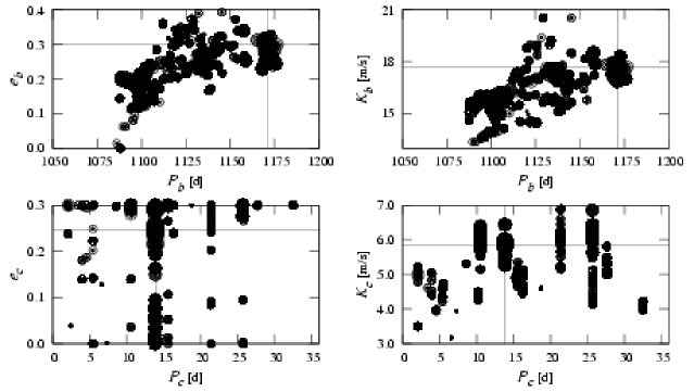
Figure 18: The parameters of the best-fits to the 2-planet model of the HD 114729 RV data projected onto the ($P,e$)- and ($P,K$)-plane. Upper plots are for the outer planet, bottom plots are for the inner companion. The values of ${(\chi^{2}_{\nu})^{1/2}}$ of the best-fit solutions are marked by the size of symbols. Largest circle is for ${(\chi^{2}_{\nu})^{1/2}}$ equal to 0.775 (the best-fit solution, Table 1); smaller symbols are for 1$\sigma$ solutions with ${(\chi^{2}_{\nu})^{1/2}}\in[0.775,0.83)$, 2$\sigma$ solutions with ${(\chi^{2}_{\nu})^{1/2}}\in[0.83,0.915)$ and 3$\sigma$ solutions with ${(\chi^{2}_{\nu})^{1/2}}\in[0.915,1.02)$ (smallest, filled circles), respectively.

An inspection of the LS periodogram shows some other relatively strong peaks, for instance about of 180 d, which most likely are aliasing with the period of $13.844$ d.

Figure 19: Lomb-Scargle periodogram of the residuals of the long-period singal in the HD 114729 data.

Figure 20 is for the histogram of ${(\chi^{2}_{\nu})^{1/2}}$ obtained for scrambled residuals of the outer planet’s signal. The probability that the residual signal of the outer companion has a random origin is very small, $p_{{\mbox{\scriptsize H}}}\simeq 0.003$. The ${(\chi^{2}_{\nu})^{1/2}}$ for the best-fit solution has well defined minimum about of 0.77. Its rms of $\sim 3.6$ m/s is very close to the mean of the internal errors. Assuming that the mass of the host star is equal to $0.93\leavevmode\nobreak\ M_{\sun}$, the derived minimal mass of the inner planet is about of $0.065m_{{\mbox{\scriptsize J}}}$ and its semi-major axis $\simeq 0.11$ AU. Thus it would correspond to a hot Neptune-like planet.

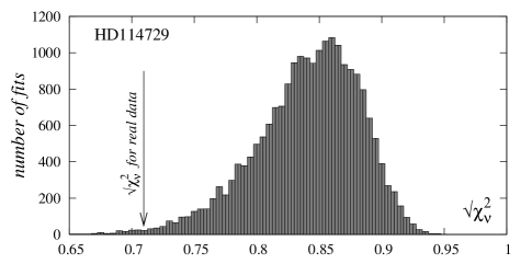
Figure 20: A histogram of ${(\chi^{2}_{\nu})^{1/2}}$ for Keplerian fits to 21,000 sets of scrambled RV residuals of the synthetic signal of the outer planet in the HD 114729 planetary system (Table 1). The position of the best-fit to the real data is marked with an arrow.

5 HD 147513

The last example which we examine is HD 147513. This star is observed by Mayor et al. (2004) who published 30 measurements covering 1690 d. In this case, an rms of 5.7 m/s of the 1-planet fit is comparable with the mean of measurement errors, nevertheless our attention draws an irregular scatter of the data about the synthetic RV curve, Fig. 22a. The discovery team announced a Jupiter-like planet of minimal mass 1.21 $m_{{\mbox{\scriptsize J}}}$ in $\simeq 528$ d orbit. The host star is very active ($R_{{\mbox{\scriptsize HK}}}^{\prime}=-4.4$). Following Wright (2005) we estimate its jitter $\sim 9$ m/s.

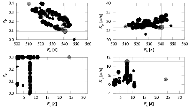
Figure 21: The projections of best-fit parameters to the 2-planet model of the HD 147513 RV data onto the ($P,e$)- and ($P,K$)-plane. Upper plots are for the outer planet, bottom plots are for the inner companion. The values of ${(\chi^{2}_{\nu})^{1/2}}$ of the best-fit solutions are marked by the size of symbols. Largest circle is for ${(\chi^{2}_{\nu})^{1/2}}\simeq 0.505$ (the best-fit solution, Table 1); smaller symbols are for 1$\sigma$ solutions with ${(\chi^{2}_{\nu})^{1/2}}\in[0.505,0.619)$, 2$\sigma$ solutions with ${(\chi^{2}_{\nu})^{1/2}}\in[0.62,0.773)$ and 3$\sigma$ solutions with ${(\chi^{2}_{\nu})^{1/2}}\in[0.773,0.95)$ (smallest, filled circles), respectively.

Figure 22: The best-fit solutions to the RV data published in (Mayor et al., 2004) for HD 147513. a) 1-planet model. The thick line is for the fit found with GA, assuming $\sigma_{j}=9$ m/s; its parameters $(K,P,e,\omega,T_{{\mbox{\scriptsize p}}}-T_{0})$ are: $(28.40\leavevmode\nobreak\ \mbox{m/s},520,49\leavevmode\nobreak\ \mbox{d},0.346,288^{\circ}.57,3125.302\leavevmode\nobreak\ \mbox{d})$, $T_{0}$=JD 2,450,000, ${(\chi^{2}_{\nu})^{1/2}}=0.737$, an rms=$6.83$ m/s. The thin line is for the fit without accounting for the jitter; its parameters are almost the same as in (Mayor et al., 2004): ($29.312\leavevmode\nobreak\ \mbox{m/s},528.112\leavevmode\nobreak\ \mbox{d},0.260,282^{\circ}.453,2214.94\leavevmode\nobreak\ \mbox{d}$), ${(\chi^{2}_{\nu})^{1/2}}=1.60$, an rms $=7.26$ m/s. b) 2-Kepler model is consistent with the measurement errors, ${(\chi^{2}_{\nu})^{1/2}}\simeq 0.505$, an rms$\simeq 4.1$ m/s. c) Period-phased RV signal of the inner companion. d) A close-up of the synthetic signal of the best-fit 2-planet configuration, Table 1.

We searched for the second planet in short-period orbit, [2,136] d. The results of the hybrid search obtained for 2-planet fits are illustrated in Fig. 21 for the statistics of the gathered best-fits and in Fig. 22a,b,c,d for the graphical illustration of the best-fit solution. These results remind us the HD 190360 case. The ${(\chi^{2}_{\nu})^{1/2}}$ of the best-fit has well defined minimum at $P_{{\mbox{\scriptsize c}}}\simeq 7.894$ d. Its rms $\simeq 4.1$ m/s means a significant improvement of the single-planet fit. This is seen in Fig. 22b,d; apparently the synthetic RV curve is ideally close to the measurements. A relatively large $K_{{\mbox{\scriptsize c}}}\sim 11$ m/s and mass of the host star $1.11\leavevmode\nobreak\ M_{\sun}$ imply the minimal mass of the inner planet $0.115\leavevmode\nobreak\ m_{{\mbox{\scriptsize J}}}$ and semi-major axis about of $0.08$ AU.

Figure 23: Lomb-Scargle periodogram of the residuals of the long-period signal visible in the RV data of HD 147513.

The LS periodogram, Fig. 23, reveals features which recall us the first system examined in this paper, about HD 208487. The short period of $\simeq 7.9$ d seems to be aliased with a much longer period of $810.8$ d. Figure 24 is for the histogram of ${(\chi^{2}_{\nu})^{1/2}}$ computed for the scrambled residuals. The probability of a random character of the residual signal is negligible. At this time, such a characteristic is almost the same as for the HD 190360 system; in that case the 2-planet solution also produces very small rms which is less than the joint measurement uncertainty.

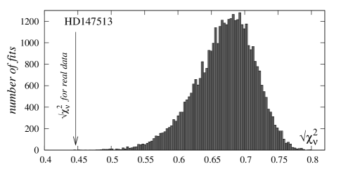
Figure 24: A histogram of ${(\chi^{2}_{\nu})^{1/2}}$ for Keplerian fits to 30,000 sets of scrambled RV residuals of the synthetic signal of the outer planet in the HD 147513 planetary system (Table 1). The position of the best-fit to the real data is marked with an arrow.

Still, mostly due to the activity of the star, the periodicity of the RV variations can be explained by jitter. According to Mayor et al. (2004), HD 147513 is a young G3/5V dwarf, only 0.3Gyr old. Its spectrum reveals a strong emission in the Ca II H line. Although the estimated short rotation period of the host star, about of 4.7 d (Mayor et al., 2004), differs from the secondary period visible in the RV signal (about of 7.9 d), it is suspiciously close to this approximation. However, such coincidence of periods still does not exclude a planetary explanation (Santos et al., 2000, 2003) because the activity can be induced or amplified by relatively massive and close planetary companion.

Table 1: Primary parameters of the model Eq. 1 and inferred elements of the best-fits found in this paper, $T_{0}$ is JD 2,450,000. See the text and figures for error estimates.

	HD 188015		HD 114729		HD 147513		HD 190360		HD 208487
Parameter	c	b	c	b	c	b	c	b	c	b
$M_{\star}$ [$M_{\sun}$]	1.08		0.93		1.11		0.95		0.96
$m\sin i$ [M${}_{{\mbox{\scriptsize J}}}$]	0.076	1.81	0.066	0.88	0.115	1.15	0.064	1.62	0.121	0.46
$a$ [AU]	0.08	1.22	0.11	2.12	0.08	1.35	0.13	3.93	0.11	0.49
$P$ [d]	8.389	476.23	13.849	1171.19	7.894	541.00	17.104	2908.32	14.496	129.51
$K$ [m/s]	7.21	44.75	5.87	17.71	10.95	26.85	5.20	24.90	10.47	19.08
$e$	0.23	0.24	0.25	0.30	0.30	0.09	0.21	0.37	0.43	0.26
$\omega$ [deg]	103.9	242.4	301.1	66.3	9.1	316.8	10.1	10.8	27.6	130.9
$T_{{\mbox{\scriptsize p}}}$ [JD-$T_{0}$]	859.67	2270.10	2496.77	1558.98	1047.23	2248.44	2370.38	3517.82	2815.87	2957.74
${(\chi^{2}_{\nu})^{1/2}}$	1.021		0.775		0.505		0.680		0.581
$\sigma{{\mbox{\scriptsize j}}}$ [m/s]	4.0		4.0		9.0		3.1		3.0
$\overline{\sigma}^{2}$ [m/s]	4.1		3.5		4.4		2.2		5.4
$(\sigma{{\mbox{\scriptsize j}}}^{2}+\overline{\sigma}^{2})^{1/2}$ [m/s]	5.7		5.3		10		3.8		6.2
rms [m/s]	4.93		3.59		4.07		2.97		2.82
$V_{0}$ [m/s]	-17.45		-3.22		-4.85		-4.81		7.97

6 Conclusions

It is extremely difficult to interpret the RV measurements when their number is limited and their time coverage is poor. We are looking for signals which have an amplitude comparable with noise. Although is already possible to pick up some promising extrasolar systems in which one planet is clearly visible and an another putative body is at the detection limit, a claim that the residual signal has a planetary origin is always very risky. To confirm the existence of the putative hot-Neptune candidates, a deep astrophysical analysis is necessary (Mayor & Queloz, 1995; Santos et al., 2003; Butler et al., 2004), by far beyond our technical abilities. That includes many additional spectroscopic and photometric observations. Nevertheless, the dynamical environment of the putative new planetary companions, several recent discoveries of Neptune-like planets and cosmogonic theories supporting their origin, permit us to state and investigate a hypothesis of the planetary nature of the RV variability.

Our results may be useful in some aspects. Even if the residual periodicities are of pure stellar origin, accounting them for may improve the single planet fits, because it makes it possible to remove a contribution of not-random RV signal from the data. When we deal with a small number of measurements, the short-term contribution of jitter does not average out and it alters the long-period solution. Yet the stellar variations may have origin in planetary-induced activity. This effect has been analyzed by Santos et al. (2000, 2003). An elimination of the planetary hypothesis also requires additional observations and analysis.

Basically, we use an independent, FFT-free method of the global analysis of the RV data and early detection of plausible planets. It can be used for checking the results of 1-dim periodogram-based analysis, extending it into the multidimensional space of the orbital elements. If some of our results will be confirmed, a similar approach can be used to detect smaller bodies in short-period orbits in the other, already discovered extrasolar systems. Such studies can be useful for planning future observing sessions.

We did a similar but very preliminary analysis of the RV observations of a few other stars hosting single Jupiter-like planets. For instance, we found a short-term variability of the RV, about of 7 d in the HD 19994 system (Mayor et al., 2004). The second companion would have $K\sim 9$ m/s, larger than the mean uncertainty of the measurements, about of 6.6 m/s. In the same paper, we found the RV data of HD 121504 and a curious RV variability which may be well modeled by a new 2-planet system close to the 6:1 mean motion resonance. Likely, the data collected and published by Doppler planet searches already hide many interesting and unusual planetary configurations.