Physical component analysis of
galaxy cluster weak gravitational lensing data

Abstract

We present a novel approach for reconstructing the projected mass distribution of clusters of galaxies from sparse and noisy weak gravitational lensing shear data. The reconstructions are regularised using knowledge gained from numerical simulations of clusters: trial mass distributions are constructed from $n$ physically-motivated components, each of which has the universal density profile and characteristic geometry observed in simulated clusters. The parameters of these components are assumed to be distributed a priori in the same way as they are in the simulated clusters. Sampling mass distributions from the components’ parameters’ posterior probability density function allows estimates of the mass distribution to be generated, with error bars. The appropriate number of components is inferred from the data itself via the Bayesian evidence, and is typically found to be small, reflecting the quality of the simulated data used in this work. Ensemble average mass maps are found to be robust to the details of the noise realisation, and succeed in recovering the input mass distribution (from a realistic simulated cluster) over a wide range of scales. We comment on the residuals of the reconstruction and their implications, and discuss the extension of the method to include strong lensing information.

1 Introduction

Mapping the mass distributions of galaxy clusters via their weak gravitational lensing effect has become something of a standard tool in astrophysics, allowing these most massive objects to be better understood in terms of their matter content, dynamical state and their value as galaxy evolution laboratories and cosmic observatories. Given this importance, it seems worthwhile to investigate  more accurate, more robust, and more practically useful methods for reconstructing the mass distributions in clusters from the available data.

Following a number of seminal papers on the subject in the 1990s (e.g. Tyson et al., 1990; Kaiser & Squires, 1993), the emphasis now is very much on the application of mapping methods to weak gravitational lensing shear data. Large CCD mosaic cameras such as SuprimeCam at Subaru, MegaCam at CFHT and the ESO Wide Field Imager at La Silla have enabled the mass distributions of clusters to be mapped to much larger radii than before (e.g. Clowe & Schneider, 2002; Broadhurst et al., 2005). From space with HST, the same science has been made possible in higher redshift clusters, first though large multi-pointing WFPC2 datasets (e.g. Hoekstra et al., 2000; Kneib et al., 2003) and subsequently with observations with the Advanced Camera for Surveys (ACS) (e.g. Lombardi et al., 2005; Jee et al., 2005). As is always the case in astronomy, these data are being pushed to their limits: the aim now is to understand cluster mass distributions in great detail, moving beyond the simple mass estimates of the early years. Kneib et al. (2003) and Gavazzi et al. (2003) measured the outer logarithmic slope of the density profile in two systems, while Clowe et al. (2004) investigated the relative peak positions of the gravitating mass density and the intracluster gas density (the latter being derived from the X-ray surface brightness). The quantification of the substructure in galaxy clusters is a topic of ongoing research, with progress being made in the central parts of clusters by comparing strong and weak lensing mass models with predictions from N-body simulations (Natarajan & Springel, 2004).

Despite the advances in data quality, weak gravitational lensing data remains very sparse and very noisy. It is notable indeed that the most exciting results in the field in recent years have come from the comparison of weak lensing data with external observations, such as the modelling of strong gravitational lensing features (e.g. Kneib et al., 2003; Bradač et al., 2005), the X-ray emission (as in Clowe et al., 2004), and the optical data on the cluster member galaxies (e.g. Czoske et al., 2002; Kneib et al., 2003). With this in mind, we ask how best to extract as much information as possible from the weak lensing data, and how to draw the most meaningful conclusions about the mass distributions in clusters. In general terms, including information from external sources means assigning appropriate prior probability distributions to whatever set of parameters we are using: to this end we seek a flexible fitting algorithm that is able to cope with such constraints and return parameter estimates (with accurate uncertainties) that reflect all the observational data in hand. Moreover, the choice of model itself can be made so as to facilitate comparisons with independent observations. However, in the first instance, it seems sensible to postpone combination with other observational data until the lensing signal is understood.

In all weak lensing reconstruction algorithms to date the assumed model has been that of a grid of pixels, whose values (be they surface mass density or lens potential) comprise the model parameters, an approach often described as “non-parametric.” It is not at all clear that a grid of pixels is the optimal model for a cluster mass distribution; as shown in Marshall et al. (2002, hereafter M02), such a large number of parameters is very often discouraged by the data quality, leading to over-fitting and potentially over-interpretation of the data. In M02, the effective number of parameters was reduced by including the assumption of the mass pixels being correlated on some characteristic angular scale ($\sim 1\;$arcmin), an algorithm implemented in the LensEnt2 code. This assumption led to smoother, less noisy maps, which, by virtue of the resolution scale being inferred from the data themselves, were restricted to show only “believable” structures with angular scales greater than the resolution parameter. In this work we seek a more natural basis set of functions with which to model cluster mass distributions. By correlating pixels together, cluster-like structures can be more easily modelled: the logical extension of this idea is to build up a mass distribution from components that already have cluster-like properties. This is the principal concept in this work.

From N-body simulations we expect the ensemble average mass distribution to be ellipsoidal with an NFW profile (e.g. Navarro et al., 1997; Jing & Suto, 2002), and clusters to lie at the high mass end of a hierarchy of structures, each with this same universal profile. The NFW profile has some support from the data, at least for the most massive halos: previous gravitational lensing analyses have found the NFW profile mass distribution to provide a somewhat better description of the data than competing models (e.g. Clowe & Schneider, 2002; Kneib et al., 2003; Gavazzi et al., 2003), as have high resolution X-ray studies (e.g. Allen et al., 2002).

If all the mass in clusters of galaxies were distributed exactly in ellipsoidal NFW-profile halos, then the optimal basis set for the lensing inverse problem would be a collection of ellipsoidal NFW profile mass components, shifted and scaled to match the various mass clumps in the field. The results of the simulations suggest that clusters do indeed look like this, and it is this that motivates our choice of mass model. This basis set allows a continuously multi-scale mass map to be reconstructed, with the angular resolution reflecting the local data quality and signal strength, but also the expected density profile cusps and slopes. We anticipate that such a basis set will be able to cope much better with the high level of noise in the data, provided that the data themselves are used to select the appropriate number of mass components used in the inference: if the weak shear data only support the inference of a small number of parameters associated with a small number of mass components, then we must be able to quantify this statement, and so automatically prevent the over-fitting that can plague pixel-based methods.

While it is the NFW component parameters that are to be inferred, it is a reconstructed projected mass map that best encapsulates our state of knowledge of the cluster potential. Such maps can be constructed by tabulating the inferred (shifted and scaled) basis functions onto a grid of pixels. These maps will have, by design, highly correlated pixel values: the covariance of the pixel values should also be taken into account to make the maps quantitatively useful.

The general ideas introduced above, whilst not previously applied in the field of weak gravitational lensing, are not new to the inferential science community. Such “atomic” methods were suggested and developed for image reconstruction by Skilling (1998), who was motivated to move beyond pixellised models when analysing spectral and image data for the same reasons as outlined above. Skilling’s “atoms” were often very simple in nature, as he sought to reconstruct complex images with very little prior knowledge. To have such a natural choice of “atom,” as proposed above for galaxy clusters, is something of a rare treat. Indeed, we might instead dub the NFW halos “physical components” to emphasise their highly motivated nature. This also helps to avoid the possible confusion that may be induced by the term “atomic inference” among the readership of this journal.

However, we should remain open to the idea that the details of the component properties are best also determined from the data – how else would we learn that the numerical simulations are realistic? In this work we demonstrate the use of NFW halos in modelling weak lensing data: alternative models may not have such well-defined prior distributions, which puts them at a natural disadvantage when comparing models. However, if a particular dataset demands a different profile atom then this can be straightforwardly inferred from the data (Kneib et al., 2003).

The methodology in this work can be rightly seen as an extension of the mass modelling of Kneib et al. (1996, and subsequent works). In their approach, one or two smooth elliptical mass components were used to model the positions of the strongly lensed images, with the parameters of the components optimised, and the model refined, as more multiple image systems were identified; the weak lensing data was used (if at all) as a weak constraint on the (primarily strong lensing) model. Here, we adopt and justify the same modelling philosophy, but focus on the weak lensing effects of lower mass substructure at larger radii, increasing the number of free parameters, automating their estimation, exploring parameter degeneracies and pushing the interpretation of the mass components beyond that of simply stating a best-fit parameter set. Indeed, our method is much closer to the “smooth particle inference” approach put forward for X-ray data analysis by Peterson et al. (2005): the differences in this case arise from the much lower signal-to noise weak lensing data (and the correspondingly fewer parameters the data can support), and the more obvious choice of basis set.

Having introduced the relevant concepts, we present in Section 2 a detailed description of the application of the atomic inference technique to weak gravitational lensing data and demonstrate its performance on simulated data in Section 4; its application to HST data is presented in  Kneib et al. (2003, to some extent) and in Jaunsen et al (2006, in prep.).

2 Methodology

2.1 Weak lensing background

The data considered here are the ellipticities of $N$ background galaxies; under the assumption of intrinsically randomly oriented galaxies, the average ellipticity provides a (noisy) estimate of the local gravitational reduced shear $g$ (see e.g. Schneider, 2006, for an introduction). The magnitude of the (complex) ellipticity, as used throughout this paper, is $|\epsilon|=(1-q)/(1+q)$ where $q$ is the ellipse axis ratio. In practice, each of $2N$ lensed ellipticity components $\epsilon_{j}$ (real and imaginary) are assumed to have been drawn independently from a Gaussian distribution with mean $g_{j}$; here $g_{j}$ is the true value of the $j^{\rm th}$ component of the (complex) reduced shear at the position of the galaxy. The likelihood function can then be written as (see e.g. Schneider et al., 2000, M02)

$${\rm Pr}(\boldsymbol{d}|\mathbf{x})=\frac{1}{Z_{\rm L}}\exp\left(-\frac{\chi^{2}}{2}\right),$$ (1)

where $\boldsymbol{d}$ is the vector of ellipticity (component) values, and $\mathbf{x}$ are the parameters of the lens potential used to calculate the shear fields at the background galaxy positions. $\chi^{2}$ is the usual misfit statistic

$$\chi^{2}=\sum_{i=1}^{N}\sum_{j=1}^{2}\frac{(\epsilon_{j,i}-g_{j,i}(\mathbf{x}))^{2}}{\sigma^{2}},$$ (2)

and the normalisation factor is

$$Z_{\rm L}=(2\pi\sigma^{2})^{\frac{2N}{2}}.$$ (3)

The effect of errors introduced by the galaxy shape estimation procedure have been included by adding them in quadrature to the intrinsic ellipticity dispersion,

$$\sigma=\sqrt{\sigma^{2}_{\rm obs}+\sigma^{2}_{\rm intrinsic}[1-{\rm max}(|g|^{2},1/|g|^{2})]^{2}}.$$ (4)

This approximation rests on the assumption that the shape estimation error $\sigma^{2}_{\rm obs}$ is Gaussian. Correcting for the effect of lensing on the intrinsic ellipticity dispersion, as suggested by Schneider et al. (2000) and implemented by Bradač et al. (2004), effectively provides the correct weighting of the ellipticities of images close to the critical regions of a strong lensing cluster. Any arclets lying within the critical curves of the cluster act as estimators for $1/g^{*}$ instead of $g$ (e.g. Bradač et al., 2005): we make this correction when calculating $\chi^{2}$. In practice very few galaxies are affected by this correction, since most lie well outside the critical region, but these are the ones that contain high lensing signal and so should be treated with care. For a projected mass distribution $\Sigma(\mathbf{x})$ composed of $n$ physical components, the reduced shear at position $\boldsymbol{\theta}$ is given by

$$g(\boldsymbol{\theta})=\frac{\sum_{k=1}^{n}\gamma^{k}(\boldsymbol{\theta})}{1-\sum_{k=1}^{n}\kappa^{k}(\boldsymbol{\theta})},$$ (5)

where $\gamma^{k}$ and $\kappa^{k}$ are the shear and convergence due to the $k$-th component, e.g.

$$\kappa^{k}(\boldsymbol{\theta})=\frac{\Sigma^{k}(\boldsymbol{\theta})}{\Sigma_{{\rm crit},i}}.$$ (6)

(See, e.g., Schneider, 2006, for more details on the weak lensing observables.) The (lens and source redshift-dependent) critical density for the $i^{\rm th}$ galaxy is $\Sigma_{{\rm crit},i}$ – any redshift information can be included here, although non-neglible redshift errors would need to be absorbed into the likelihood function, broadening it somewhat.

Note that in the above model all mass components are assumed to be at the same redshift. This is both necessary for the thin lens plane formulae to be applicable, and appropriate for a cluster modelling algorithm where all mass in the field of view is assumed to be associated with the cluster. If there were massive clumps lying along the line of sight their gravitational shear effects would be interpreted within this model. Extending the physical component analysis into three dimensions is an intriguing possibility but beyond the scope of this paper; however we do note that it may be profitable to do so, as the additional information needed in constraining the redshift of the components, and the more complex lens equations needed to predict the observed shear, are both readily incorporated into the already non-linear data model.

2.2 The physical component (halo) mass model

In the spherically symmetric case the NFW density profile (Navarro et al., 1997) is

$$\rho(r)=\frac{\rho_{\rm s}}{\left(r/r_{\rm s}\right)\left(1+r/r_{\rm s}\right)^{2}},$$ (7)

where $r_{\rm s}$ and $\rho_{\rm s}$ are the radius and density at which the logarithmic slope breaks from $-1$ to $-3$. It is useful to normalise this profile, which we treat as a two-parameter fitting function, to the mass contained within a region of overdensity 200 relative to the critical density at that redshift  (Allen et al., 2003; Evrard et al., 2002):

$$\frac{M(r_{200})}{\frac{4}{3}\pi r_{200}^{3}} =200\rho_{\rm crit}$$ (8)

$$=4\pi\rho_{\rm s}r_{\rm s}^{3}\left[\log{(1+c)}-\frac{c}{1+c}\right].$$ (9)

Here, $c=r_{200}/r_{s}$ is a measure of the concentration of the halo. Lensing properties of the NFW model have been worked out by a number of authors (Bartelmann, 1996; Wright & Brainerd, 2000; Meneghetti et al., 2003) and we do not reproduce their results here. Each NFW mass component contributes to the shear field: we assign a uniform prior distribution to the component positions within the observation region.

It has been found in many previous lensing analyses that it is rather important to include the ellipticity of the lens (see e.g. King et al., 2002; Sand et al., 2004; Kochanek, 2006). There is some choice as to whether the lens potential, the deflection angle or the surface density should be asserted to be elliptically symmetric – since the three quantities differ by the number of times the gradient operator has been applied (0, 1 and 2 times respectively), only one of them can have concentric elliptical contours. King & Schneider (2001) chose the surface density, while Golse & Kneib (2002) opted for the slightly rectangular projected mass contours of a concentric elliptical deflection angle distribution. We follow Meneghetti et al. (2003) and, citing analytic tractability, use the lens potential $\psi(\boldsymbol{\theta})$: the major disadvantage of this approach is that for axis ratios of less than $\approx 0.7$ the corresponding mass distribution becomes dumbbell-shaped. However, massive cluster potentials are likely to be much closer to spherical than this: we quantify this point below. The breaking of axial symmetry means that the derivatives of the lens potential must be calculated explicitly in order to calculate the shear and convergence; this can be done analytically for each NFW profile component. In this process the radius parameter is defined in such a way as to keep the mass within a given circular radius constant as the ellipticity changes (e.g. Kassiola & Kovner, 1993; Meneghetti et al., 2003).

As outlined in the introduction, N-body simulations provide the prior probability distributions for the NFW profile parameters. For example, Jing & Suto (2002) showed that numerically simulated cluster-scale halos can be reasonably well modelled using triaxial ellipsoidal density profiles, and produced fitting functions for the probability distributions of the two axis ratios. However, as indicated above, we prefer to use the more readily calculated elliptical lens potential: we use the following procedure to derive an approximate prior on the lens potential ellipticity parameter from the distributions tabulated by Jing & Suto.

We draw a large number of halos’ axis ratios from the fitted joint probability density function (PDF), numerically project the prescribed densities onto the lens plane, and then compute (using, after padding with zeros, fast Fourier transforms – FFTs) the corresponding lens potentials via the convolution

$$\psi(\boldsymbol{\theta})=\frac{1}{\pi}\int\kappa(\boldsymbol{\theta}^{\prime})\log|\boldsymbol{\theta}-\boldsymbol{\theta}^{\prime}|d^{2}\boldsymbol{\theta}^{\prime}.$$ (10)

We then measure the axis ratio of the resulting isopotentials, from the ratios of the second moments of the potential. These isopotentials are not quite elliptical, and the inferred ellipticity changes slightly with radius; however the derived ellipticities were compared with the actual isopotential at the scale radius and found to deviate by only a few percent. The resulting derived probability distribution for the lens ellipticity, defined as in Section 2.1, is given in Figure 1. It is well-approximated by a Gaussian distribution with mean 0.125 and width (standard deviation) 0.05, and it is this that we use as our ellipticity prior. The effects of this prior are to suppress halos with unphysically high ellipticity, and to favour the non-spherical halos which are more commonly seen in the N-body simulations. The position angle of the halo is assumed to follow a uniform distribution between $0$ and $180$ degrees: in the two-dimensional ellipticity component space the prior PDF peaks at the circularly symmetric model.

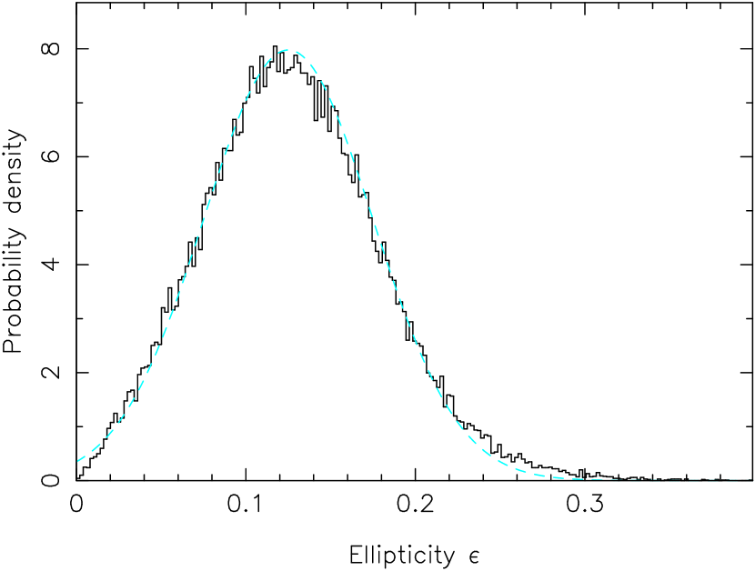
Figure 1: Prior PDF for the (modulus of the) lens component isopotential ellipticity, derived from fits to a statistical sample of N-body simulated clusters by Jing & Suto (2002). The dashed curve is a Gaussian distribution of mean 0.125 and width 0.05.

The priors on the NFW profile parameters may also be derived from N-body simulations. For example, Jing & Suto (2002) find the concentration parameter $c$ to be distributed log-normally with width $\approx 0.3$ about a value of 3, for a massive cluster at redshift 0.5. We note that this width corresponds to an uncertainty of $\approx 50\%$. Although much larger values of the concentration have been inferred in some lensing analyses (Kneib et al., 2003; Gavazzi et al., 2003), it is not clear that the data have enough constraining power in the critical region to support this conclusion. In any case, a concentration of 20 is less than 3-sigma from the mean of the lognormal distribution, suggesting that this prior is flexible enough to cope with unusual concentrations (whilst retaining the desired feature of rejecting very low, and indeed negative, values).

Finally we consider the prior on the atom mass itself, $M_{200}$. The Press-Schecter formalism (Press & Schechter, 1974), or one of its many numerically-corrected forms (e.g. Jenkins et al., 2001; Evrard et al., 2002), would serve to provide an approximate prior PDF for the halo mass were we observing a random patch of sky. The logarithmic slope of the mass function at the mass scale of galaxy clusters is close to $-2$, indicating the rareness of massive clusters. However, we are interested in pre-selected clusters, whose masses are large and typically estimable to within an order of magnitude. We suggest a compromise, and assign a Jeffreys prior PDF (logarithmic slope $-1$) to the halo mass, sampling uniformly in the logarithm of the mass. This has the pleasant effect of suppressing the introduction of mass into the map unless it is required by the data, but is not so severe that the halos either have masses that are heavily biased low, or are discouraged completely. A more rigorous approach would be to use the predicted halo occupation distribution to provide a joint prior on the number and mass of sub-halos, given a main cluster component. This is beyond the scope of this paper: the specified priors suffice to define a robust data model. We will see in Section 3 that the method is somewhat insensitive to the exact form of this prior, with the presence of components, and their masses, being principally determined from the data.

2.3 Parameter inference

Whilst linear methods are often favoured on the grounds of computation speed and ease of error propagation, we argue that the benefits of a fully non-linear fit outweigh these factors. We are seeking an optimal mass reconstruction, folding in as much information as we can: we do not wish to compromise this goal in favour of a computationally easier alternative. With the non-linearity comes flexibility: introducing new constraints on the mass distribution can be done in a conceptually straightforward way, adding extra terms to the posterior PDF for the model parameters.

In the non-linear data model the global best-fit point is typically hard to find, and exists in a parameter space whose dimensionality can run well into double figures when many components are used. To solve these problems we employ a Markov chain Monte Carlo (MCMC) sampler to explore the parameter space. This technique is now widespread in astronomical data analysis (see e.g. Knox et al., 2001; Lewis & Bridle, 2002; Marshall et al., 2003; Dunkley et al., 2005; Bonamente et al., 2004; Peterson et al., 2005, for some examples of its use). Good introductions to the technique are given by Gilks et al. (1996) and MacKay (2003); here we make the following brief comments.

Having defined a likelihood function ${\rm Pr}(\boldsymbol{d}|\mathbf{x},n)$, and sensible priors ${\rm Pr}(\mathbf{x})$ on the parameters $\mathbf{x}$ of the $n$ mass components, we note that the distribution containing all the information about the mass distribution is the posterior PDF:

$${\rm Pr}(\mathbf{x}|\boldsymbol{d})=\frac{{\rm Pr}(\boldsymbol{d}|\mathbf{x},n){\rm Pr}(\mathbf{x})}{{\rm Pr}(\boldsymbol{d}|n)}$$ (11)

Calculating the numerator of the right hand side on a fine grid throughout the parameter space would allow the normalising evidence ${\rm Pr}(\boldsymbol{d}|n)$ to be calculated, the regions of high probability to be located, and any uninteresting parameters to be numerically integrated over. In any more than a few dimensions both these operations are computationally unfeasible. It is much more convenient to work with samples drawn from the posterior distribution: both marginalisation and changing variables are trivial, the latter being done on a sample-by-sample basis. MCMC provides an efficient way of drawing these samples.

Perhaps of greater practical importance is the robustness of MCMC to local maxima in the likelihood. Optimisation schemes for locating the best-fit point are vulnerable to becoming trapped at the wrong point in parameter space: MCMC alleviates this problem by providing a way out of such traps (i.e. with a random trial step to a nearby part of the parameter space).

Note the dependence of the likelihood and evidence on the number of components used in the model, $n$ (the priors on each component’s parameters having been chosen to be independent of $n$). The posterior probability distribution for $n$ can be seen to be available from the data via the evidence: ${\rm Pr}(n|\boldsymbol{d})\propto{\rm Pr}(\boldsymbol{d}|n){\rm Pr}(n)$. With the assignment of a uniform prior on the number of components, the evidence gives the (discrete) PDF for $n$ directly. In the same way the evidence may also be used to quantify the relative probabilities of two or more competing component models, a process carried out in Kneib et al. (2003). The evidence lies at the heart of all Bayesian model selection and hypothesis testing (see e.g. MacKay, 2003, for an excellent introduction), and its use is growing in astronomy (e.g. Jaffe, 1996; Knox et al., 1998; Hobson et al., 2002; Marshall et al., 2003; Mukherjee et al., 2006).

We use the freely available software package bayesys3, written by John Skilling. This general purpose code, used in previous work on this subject (Marshall et al., 2003), is known to cope well with the types of likelihood surface presented by weak lensing datasets: we find the evidence values to be accurate and their calculation readily repeated. The evidence is calculated by thermodynamic integration during the burn-in period (Ó Ruanaidh & Fitzgerald, 1996).

The only disadvantage to using MCMC rather than an optimisation followed by a Gaussian approximation to the posterior is that it can be slow: typically, analysing a catalogue of some few thousand galaxies using a model consisting of three components on a 3GHz processor can be expected to take several hours, while a chi-squared minimisation may only take minutes. However, the problem of avoiding local posterior maxima typically leads one to consider an ensemble of minimisations from different starting points, or the use of some more advanced algorithm such as simulated annealing (which incur many more likelihood evaluations). Likewise, estimating uncertainties is commonly done using techniques such as bootstrap re-sampling or simulation of mock data. The MCMC process performs more or less the same calculation during the inference. Therefore it is the total run time, to obtain both reliable parameter estimates and their uncertainties that should be compared between methods – with this metric MCMC becomes rather competitive.

2.4 Probabilistic mass mapping

While the parameters of individual halos may well be of interest (e.g. Kneib et al., 2003), the information on the mass distribution can be displayed in a more visually helpful way, in the form of a mass image. Each MCMC sample corresponds to a set of halos that provide an acceptable fit to the data: the projected mass distribution of these halos can be mapped on to a pixellised grid. The probability distribution of the surface mass density in any given pixel can be built up by calculating its value for each sample, and forming a histogram. This is the PDF marginalised over all halo parameters, so that the width of this distribution represents the maximum uncertainty of that pixel value, given the assumptions. To make a map, the individual pixel probability distributions have to be reduced to one number: we use the arithmetic mean for its ease of calculation (Skilling, 1998), but note that an alternative central value may be more appropriate if the pixel value PDF is highly skewed.

The resulting reconstructed maps inevitably retain some of the appearance of the halos from which they are composed: however, averaging over the posterior PDF does bring out some extra information not present in any individual sample map. These reconstructions can be thought of as having been highly regularised, using a multi-scale kernel whose shape has been chosen to be appropriate for dark matter in cluster halos. In the next section we show some examples of these atomic maps, and how well they describe the lensing data.

3 Demonstration on simulated data

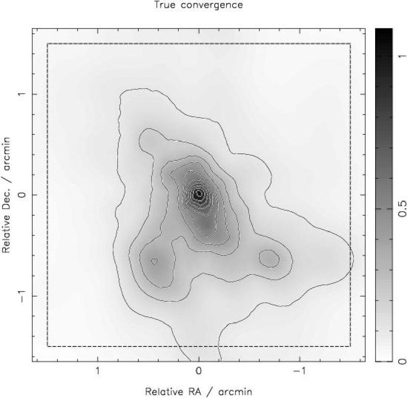
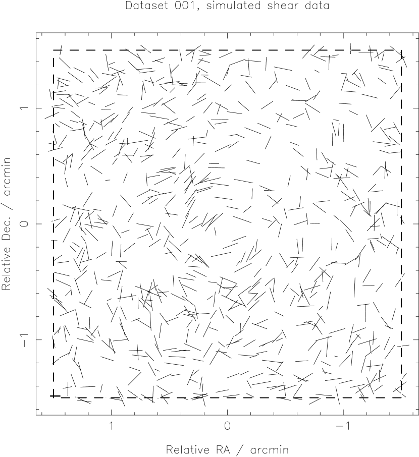
Figure 2: True convergence distribution (left) and mock ellipticity data (right) for the $z=0.55$ N-body simulated cluster described in the text, assuming a source plane redshift of 1.2. The 3-arcmin square observing region is shown by the dashed box. One main clump, and two minor clumps, are visible in the mass map.

In order to demonstrate the methodology introduced above, we generated mock weak lensing data for a typical, moderately massive ($M_{\rm virial}\approx 6\times 10^{14}M_{\odot}$), unrelaxed cluster at redshift 0.55. We used an N-body simulated cluster, from the sample in Eke, Navarro & Frenk (1998). We placed background galaxies at random positions on a single source plane at redshift 1.2 (such that the cluster has a tangential critical curve with radius $\approx 5$ arcsec), with a number density of 80 per square arcmin over a square field 3 arcmin on a side. This was intended to represent a standard weak lensing dataset from the ACS camera on HST, and resulted in a catalogue of 741 galaxy shapes. An intrinsic ellipticity distribution of width 0.25, and shape estimation error of 0.2, were assumed. The reduced shear due to the input cluster was calculated by convolving (using FFTs) the simulated cluster mass distribution (as provided by the simulators and after padding with zeros to avoid edge effects) with the lensing kernel, and then scaling by the critical density, as in Marshall et al. (2002). We note that this process used a projected density map with pixel scale $\approx 2$ arcsec, fine enough to retain any cuspy features in the mass distribution.

When assessing the statistical performance of the atomic inference algorithm, multiple noise realisations were used. Each realisation corresponds to a separate set of background galaxy positions and intrinsic ellipticities, and a different shape estimation noise term. The true projected mass distribution, scaled by the critical density for this lens and source redshift, is shown in Figure 2, along with one realisation of the simulated weak lensing data.

A single source plane was employed for simplicity, and to separate out the performance of the atomic modelling from systematic effects due to unknown background galaxy redshifts. We do note again, however, that including measured redshifts for each source is trivial in this algorithm, since we predict the convergence and shear at each background galaxy position.

3.1 Estimating the number of halos

We first investigate the number of halos appropriate for modelling this mock dataset. This was done by sampling the posterior distributions of the parameters of an $n$-component model, where $n$ was allowed to increase from 1 to 5. For each inference, the evidence was calculated, and is shown in Figure 3. These evidence values are readily reproducible, as indicated by the error bars on the plot: these show the standard deviations of the mean log evidence, over 5 runs of the sampler, to be routinely less than one unit. This plot gives us some confidence in the ability of the sampler to simulate the posterior PDF; it also quantifies the quality of the data available in observations such as that simulated. The plot shows evidence curves from ten different noise realisations, all of which peak at between 1 and 3 components. The different noise realisations give rise to posterior probability distributions with different geometries and complexities: the different challenges thus presented to the sampler result in a range of error bar sizes. In contrast, the scatter between the curves shows the effect the noise has on the appropriateness of $n$ components.

The evidence for the $n$-halo model is ${\rm Pr}(\boldsymbol{d}|n)$: the ratio of this to the evidence for zero atoms (i.e. the null model, with zero predicted surface mass density) gives a measure of the significance of the detection (Hobson & McLachlan, 2003). Had Figure 3 been plotted over a wider range in the ordinate, probability (evidence) ratios relative to the null model of ${\rm e}^{40-60}$ would have been visible, indicating a resounding detection of the cluster in the shear data. The differences between evidence values for $n$ of 1, 2, 3, 4 and 5 components are much smaller, typically reaching between two and four units in the logarithm between the peak evidence and the $n=5$ value. These differences correspond to probability ratios of approximately $10-50$: the data are found to be typically an order of magnitude more likely to have come from a two-component model than a 5-component model (with the exact favoured value of $n$ being dependent on the noise realisation). This is an important result: the simulated data were designed to be representative of that being analysed in contemporary work; what we are seeing here is a quantification of the amount of information available to us from that data. With the well-appointed halo model used, only a handful of parameters are both required and supported by the data. This is in agreement with the findings of M02: in the next section we show how the inferred mass distributions differ from the maximum entropy maps.

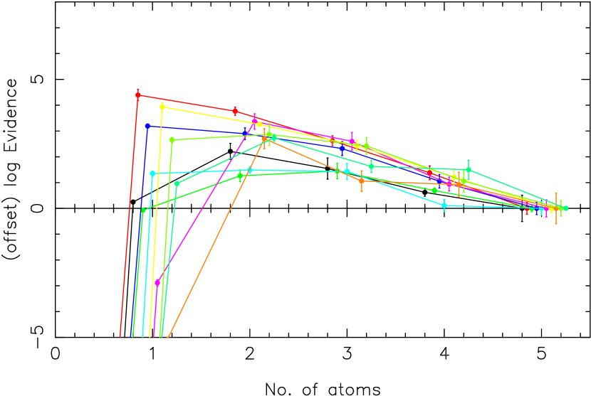
Figure 3: (Renormalised) log evidence as a function of halo number for the simulated cluster described in the text. The points with error bars show the evidence estimates at each atom number: the ten lines correspond to ten different noise realisations of the simulation. A broad peak around atom number 1-3 is typically seen.

3.2 Mass mapping

The left-hand panels of Figure 4 show the ensemble-averaged halo-model mass reconstructions, for two different noise realisations. For comparison, the maximum-entropy maps are shown along side, at two different resolution scales. These plots serve to illustrate some general points about the two techniques. The LensEnt2 algorithm, and any other method that uses a single resolution scale when smoothing the data or in the reconstruction process itself, does not cope well with the range of scales of mass structure in this cluster. A sharp, cuspy peak, surrounded by an extended irregular mass distribution in the outer regions clearly requires at least two scales (approximated here by the 15 and 40-arcsec LensEnt2 resolution kernels): these scales are provided naturally by the physical components. The “atomic” reconstruction is remarkably robust between noise realisations, whereas the more flexible pixel-based method maps contain transient structure as the noise is fitted. This problem was alleviated in M02 by increasing the resolution scale until, at maximum evidence, only believable features remained; the same may be said about the structure in the atomic maps, except that the small-scale, high signal-to-noise structure is retained (e.g. at the centre of the cluster). Finally we note the long standing problem of inferring super-critical density from weak shear data, outlined in some detail in the work of Schneider & Seitz (1995; 1995). With no additional information it is impossible to infer uniquely the presence of convergence greater than unity: in contrast, when constructing the mass distribution from naturally cuspy components the convergence can be effectively interpolated upwards in a seamless and physically-reasonable way.

The observations of the previous paragraph can be put on a more quantitative footing by plotting the correlation between the inputs and outputs of the algorithms. This is shown in Figure 5. We use the correlation function $\xi_{+}(\theta)$, where $\theta$ is the angular separation between galaxy pairs; this is given by (e.g. Schneider, 2006):

$$\xi_{+}(\theta)=\langle g_{\rm t}^{\rm A}g_{\rm t}^{\rm B}\rangle+\langle g_{\rm x}^{\rm A}g_{\rm x}^{\rm B}\rangle,$$ (12)

where $g_{\rm t}^{\rm A}$ ($g_{\rm x}^{\rm A}$) is the tangential (cross) component of the reduced shear estimator at galaxy position of galaxy A, relative to galaxy position B (and vice versa). This function conveniently quantifies the alignment of pairs of galaxy shapes. Since we are interested in the difference between the reduced shear predicted by the reconstructions ($g$), and either the true reduced shear ($\hat{g}$) or measured ellipticities ($\epsilon$), we construct the difference function

$$\Delta\xi_{+}(\theta) =\langle(g_{\rm t}^{\rm A}-\hat{g}_{\rm t}^{\rm A})(g_{\rm t}^{\rm B}-\hat{g}_{\rm t}^{\rm B})\rangle$$

$$\;\;\;\;+\langle(g_{\rm x}^{\rm A}-\hat{g}_{\rm x}^{\rm A})(g_{\rm x}^{\rm B}-\hat{g}_{\rm x}^{\rm B})\rangle$$ (13)

$$=\xi_{+}^{gg}(\theta)+\xi_{+}^{\hat{g}\hat{g}}(\theta)-2\xi_{+}^{g\hat{g}}(\theta).$$ (14)

For a perfect match on all scales, this function would be zero. All correlation functions decrease with increasing pair separation, as the lensing signal diminishes in strength. The upper panel of Figure 5 shows that the residuals in the 3-atom reconstruction, and the evidence-preferred 40-arcsec LensEnt2 reconstruction, are consistent with noise; the high resolution LensEnt2 reconstruction shows a small positive $\Delta\xi_{+}(\theta)$ at scales of 5-40 arcsec indicative of an imperfect reconstruction. This shortcoming is seen more clearly in the lower panel; in the figure the low resolution LensEnt2 map and the 3-atom reconstruction are seen to perform roughly equally well in recovering the true mass distribution, with the atomic map doing slightly better on the smallest scales. This agrees with the maps of Figure 4, where the cuspy cluster centre is not reproduced with the smooth maximum-entropy map.

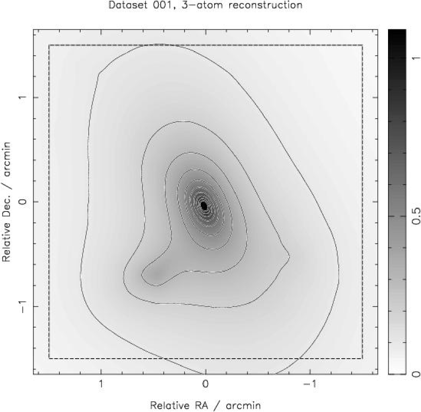
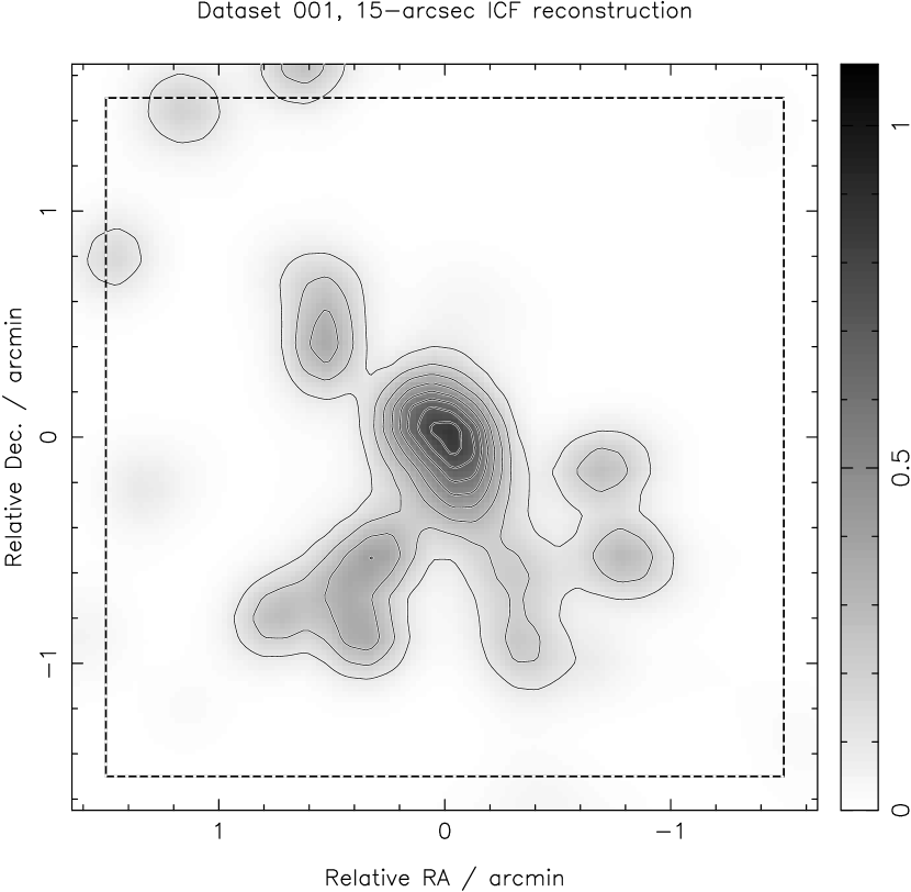
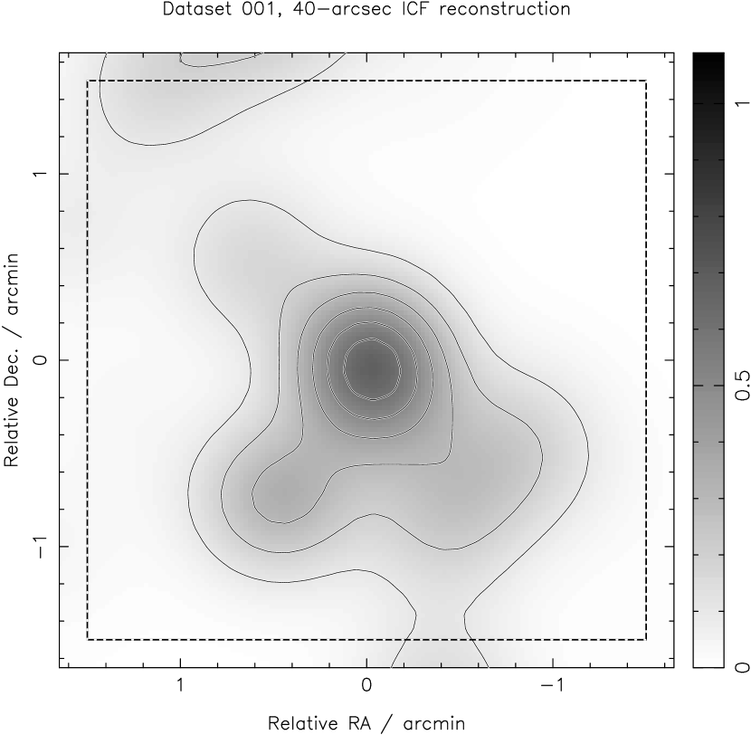
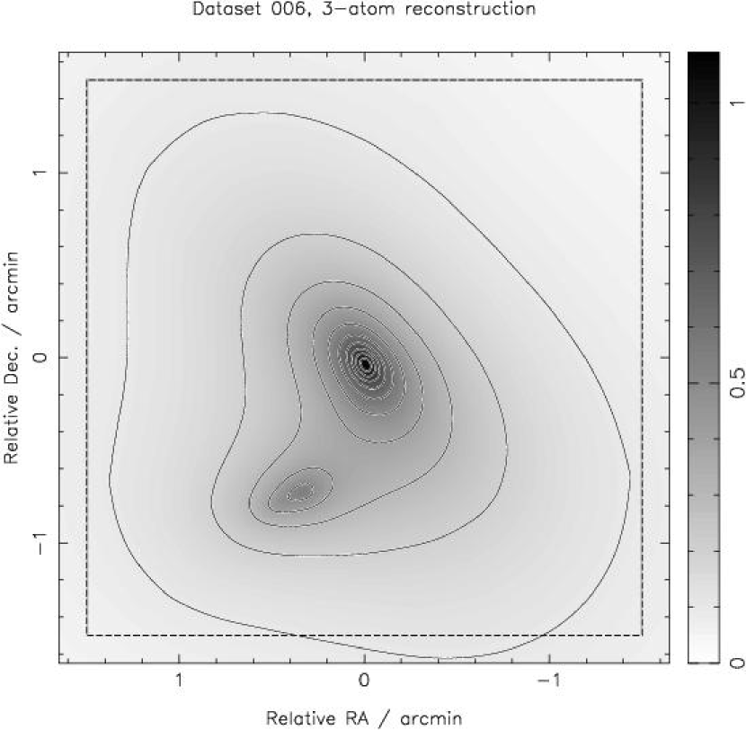
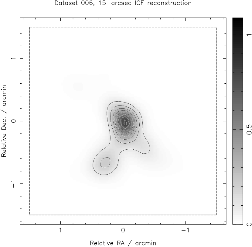
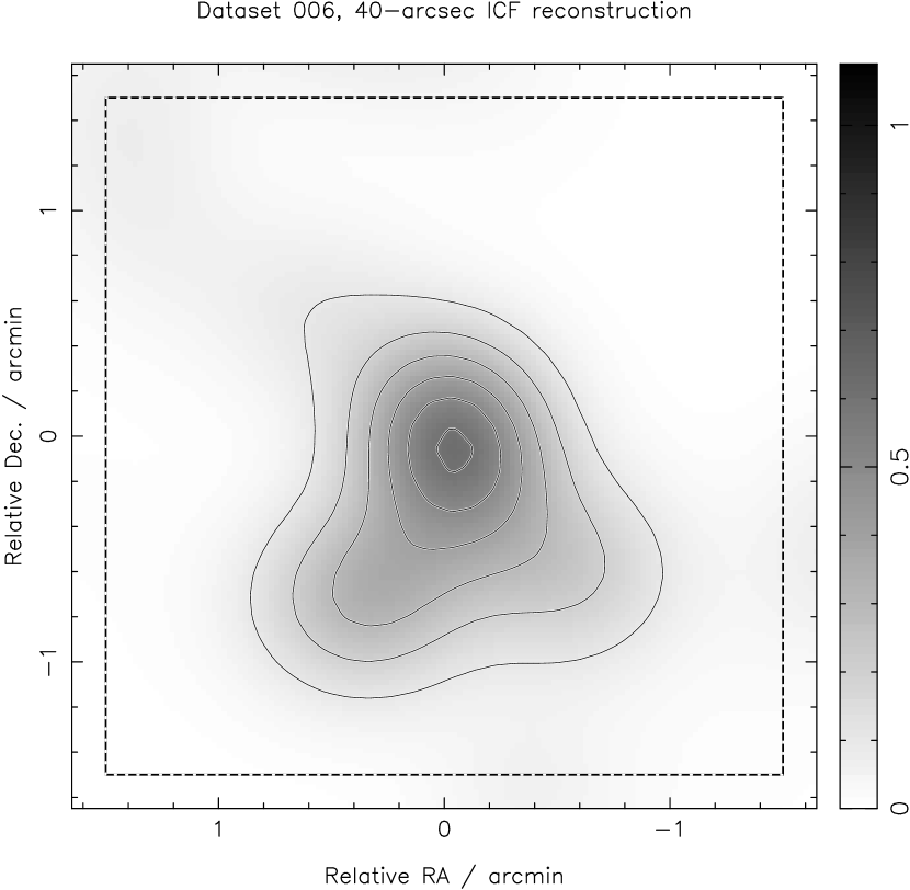
Figure 4: Two representative mass reconstructions, one noise realisation per row, for the $z=0.55$ simulated cluster described in the text. Left column: ensemble-average atomic inference mass distributions. Centre and right columns: 15 and 40-arcsec resolution maximum-entropy maps. These panels may be compared directly with the left-hand panel of Figure 2. The 3-arcminute square observing region is shown by the dashed box.

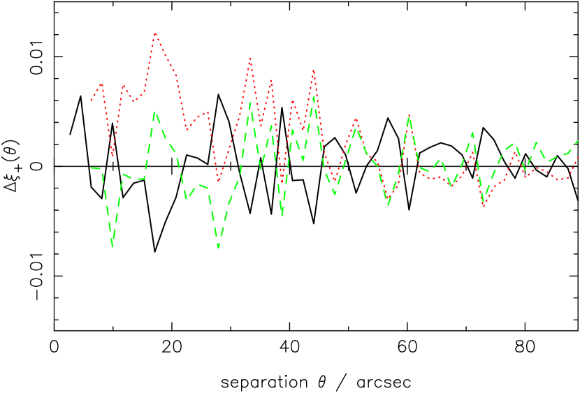
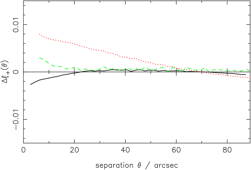
Figure 5: Quantifying the mass map reconstruction accuracy via the correlation function differences. Top: correlation function $\xi_{+}$ of the difference between the ensemble-average predicted reduced shear, and the data. The curves shown are for the 3-halo atomic reconstruction (solid), 15-arcsec resolution LensEnt2 map (dotted), and the 40-arcsec LensEnt2 map (dashed). Bottom: the same exercise, with the same legend, but now comparing the predicted reduced shear with the true input values.

The information in the correlation functions may also be visualised via maps of residuals. Plotted in the left panel of Figure 6 is the difference between the reconstruction in the top left hand panel of Figure 4, and the true mass distribution; for comparison, the central panel shows the width of the pixel value PDF, as estimated by the standard deviation of the samples. This “error” map is informative: even in the regions where the shear signal is strong, the uncertainty on the predicted convergence is high. However, using this uncertainty map to rescale the residuals between reconstruction and truth we see that the differences are fairly low significance: only in the region of the undetected sub-clump are the pixel values more than 3 sigma from the truth (where “sigma” is the uncertainty mapped in the central panel).

Evident in Figure 6 is the small-scale mass structure in the cluster core, undetectable by weak lensing, that makes pointwise convergence prediction at the level of a few percent or better very difficult. Clearly more information is needed: the work of Natarajan & Springel (2004) indicates that including the mass associated with galaxies (via small components placed at the cluster member positions) is sufficient to model this substructure.

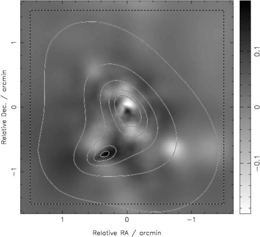
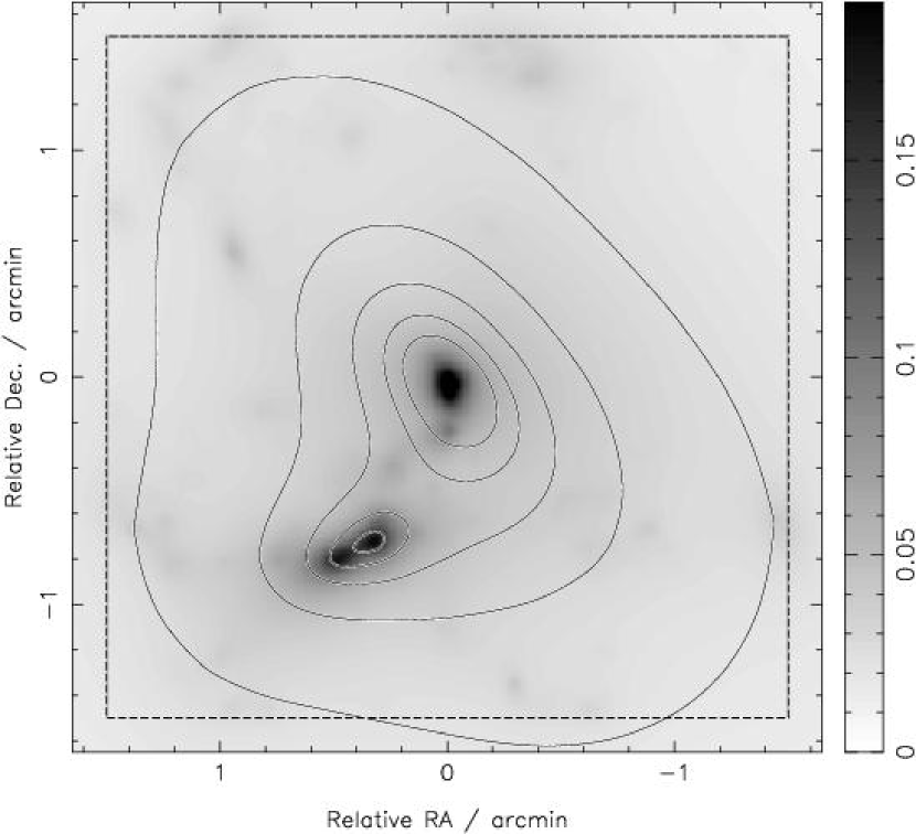
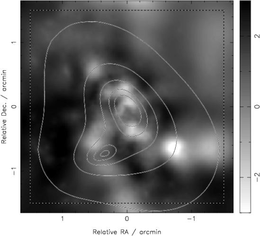
Figure 6: Left: difference map between the 3-halo reconstruction of Figure 4 and the true surface density seen in Figure 2. Centre: the physical component method uncertainty map, as estimated by the standard deviations of the individual pixel PDFs. Right: the difference map, divided by the error map. In all panels the reconstructed convergence contours are overplotted to guide the eye.

3.3 Component properties

The ensemble average mass map is one way of representing the information in the joint posterior PDF; marginal distributions for other parameters of interest are also readily available. For example, Figure 7 shows the position, and mass profile parameters, associated with the secondary sub-clump visible in the projected mass map. MCMC samples corresponding to a circular region centred on the map peak were excised and histogrammed, to plot the marginalised posterior distributions for component position ${\rm Pr}(x,y|\boldsymbol{d},H)$, and density profile parameters ${\rm Pr}(M_{200},c|\boldsymbol{d},H)$, where $H$ is the assumption that a mass feature of interest lies within this aperture. The widths of these distributions provide estimates of the uncertainties on the parameters. This secondary feature is somewhat transient: in some noise realisations the signal is too broken up to be detected.

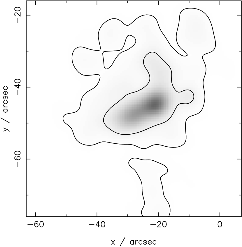
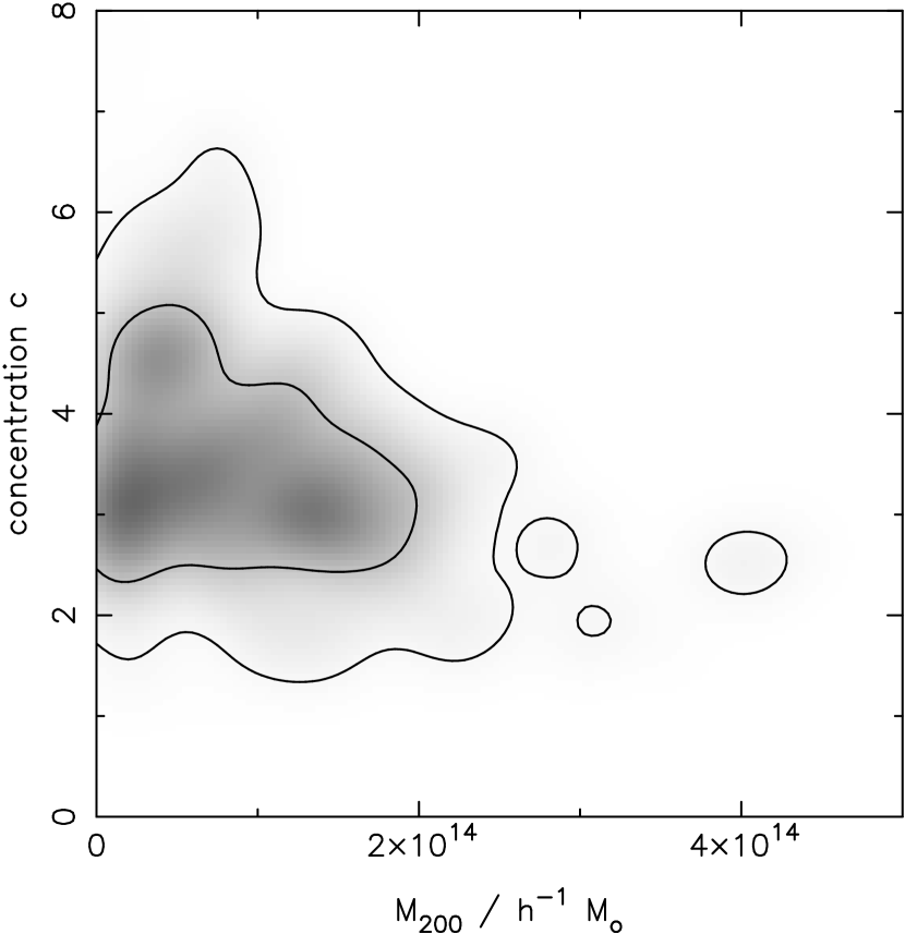
Figure 7: Inferences about the south-eastern substructure seen in the reconstruction of Figure 4. Left: ${\rm Pr}(x,y|\boldsymbol{d})$; right: ${\rm Pr}(M_{200},c|\boldsymbol{d})$. In the right panel the prior on the concentration can be seen, allowing a reasonable estimate of the mass of the marginally-detected subclump.

4 Discussion

We now discuss three of aspects of the physical component analysis in greater detail. First is the sensitivity of the method to the prior PDFs assigned to the model parameters; second is the effect of the assumed halo model on the accuracy of the reconstruction; third is the potential for including strong lensing information.

4.1 “Bias” in the reconstruction

We point out explicitly that the mass maps derived in the physical component analysis are biased, in the sense that no matter how good the data is the predicted mass distribution still has to be constructed from NFW-shaped halos, and in any individual cluster observed at a high signal-to-noise ratio one can imagine this model breaking down. Indeed, careful inspection of the maps in Figure 6 shows that the reconstructed surface density is systematically higher than the true density in the outer parts of the field of view, by 0.05 in convergence or so. This is despite the ellipticity data being fitted to a fully satisfactory level (Figure 5), and is due to the mass sheet degeneracy  (Falco et al., 1985). This effect when working with parameterised profiles was pointed out by Schneider et al. (2000) and further investigated by Bradač et al. (2004), and was left as a limitation on the measurement of cluster density profiles. In the present case we are effectively selecting a particular mass sheet transformation parameter through our choice of the NFW profile for our mass components: the error bars mapped in Figure 6 are model-dependent. The bias does lie, however, within this statistical uncertainty: the simulated cluster used here is well-fit by a density profile close to NFW!

The model-dependence of the inferences advocated is therefore presented as a sensible use of the prior information available from N-body simulations. However, one should remember that the universal profiles came from fitting the ensemble average profiles of simulated halos: in any given cluster it may be that the prior distribution for the concentration may not afford the halo profiles sufficient freedom to fit the data well, or even that some alternative profile is more appropriate altogether. In this case, the profile can be inferred from the data via the evidence as was shown in (Kneib et al., 2003). When using any other profile, the priors on the halo parameters will not be as readily derived, and indeed may be preferred to be kept uninformative. In this case the Occam’s razor factor inherent to the evidence will act to favour the basic (and a priori better-constrained) NFW atom set. A consequent increase in evidence when using the alternative profile will then be a rather robust conclusion, the analyst’s natural tendency towards the expected forms having been taken care of already.

4.2 Robustness to prior PDFs

Weak lensing data is very noisy: in such situations, we should be wary of the prior PDF becoming comparable in importance to the likelihood function. We investigated this for the simulated dataset described above by applying some alternative priors and examining the evidence values. For the component masses we tried a prior uniform in mass (as opposed to the Jeffrey’s prior suggested above, which is uniform in the logarithm of the mass). This prior is more favourable to higher mass components: if the presence of an extra component were being suppressed by the Jeffreys prior then we would be more likely to see it with the more forgiving uniform distribution. We found the Jeffrey’s prior to give slightly higher evidence, perhaps slightly better reflecting the true halo occupation distribution. The difference was however, much less than one unit, suggesting that the component number and mass are well-determined by the data. Indeed, the resulting mass maps were indistinguishable from those from the main analysis.

Connected to the prior for the component mass is that for the component number, implicitly assumed to be uniform when interpreting Figure 3. While there may be some theoretical motivation for attempting to model the cluster with a mass function, that gives a joint PDF on $n$ and halo mass, that is steeper than that used here, we would run the risk of over-fitting the data. At present, Figure 3 shows that the fit is being sensibly regularised in models with small numbers of components, with the evidence clearly decreasing towards higher $n$. When using data with artificially low noise, the evidence does indeed favour higher numbers of components, and lower mass features in the field are indeed recovered, as expected.

We also investigated the effect of changing the component ellipticity prior, broadening it to make higher ellipticity components intrinsically more probable. Again, this made very little difference to the evidence values or to the mass maps.

4.3 Including strong lensing information

The non-linear nature of the inference process described in the previous sections makes it straightforward to include strong lensing constraints as priors. These constraints may come from galaxy-scale lenses in the field, or from objects multiply-imaged by the cluster potential itself.

For example, an independent strong lens modelling (on either scale) might be designed to yield estimates of the convergence and shear (or perhaps more likely, magnification $\mu$) at a particular point, with error bars (e.g. $\sigma_{\mu}$). These uncertainties, when translated into Gaussian (or the appropriate error distribution) PDFs centred on the point estimate, can be used to weight the MCMC trial parameter sets: the weak lensing likelihood is simply multiplied by the value of a PDF such as ${\rm Pr}(\kappa|\mu,\sigma_{\mu})$. This approach, while convenient for marrying two independent pieces of analysis software, would be somewhat wasteful in its use of information (and has not yet been applied in practice!). A more rigorous approach would be to include the strong lens image positions, or even the image pixel values themselves, as data, and form a joint likelihood from the product of the individual weak and strong lensing forms. Such an analysis is beyond the scope of this work, but is being developed as an extension of the LensTool package (Kneib et al., 1996). MCMC is anticipated as being very useful indeed here: the strong lensing likelihood surface is highly complex.

One application of cluster lensing that has been suggested is to predict the “external” convergence at the position of galaxy-scale strong lenses in the cluster field (e.g. Bernstein & Fischer, 1999; Kneib et al., 2000). Any contribution to the strong lens convergence is degenerate with the estimate of Hubble’s constant from that lens, motivating the study of additional constraints on the convergence, such as might be hoped for from weak lensing. While both strong and weak lens systems suffer from the mass sheet degeneracy referred to above, when assuming physically-motivated parameterised profiles for all mass distributions this degeneracy is broken. A model-dependent estimate of convergence at a particular point in the field (and indeed its posterior probability distribution) can then be generated from the MCMC samples: its accuracy will be dependent on both the noise in the weak lensing data, and the assumptions of an NFW-profile component cluster. The maps in Figure 6 suggest that, for the data quality investigated here, both the statistical and systematic parts of the error bar on a pointwise convergence estimate are likely to be in the region of 0.05, representing a significantly greater fractional error than that due to the best-measured time delays.

5 Conclusions

We have presented a new method for reconstructing the mass distribution of clusters of galaxies from weak gravitational lensing data, based on the atomic inference procedure suggested by Skilling (1998). By investigating its performance on simulated HST ACS data, we draw the following conclusions:

• Perhaps as expected, the number of mass components supported by the data (and selected via the evidence) is typically quite small. This is a consequence of the domination of clusters by a single deep potential with a few satellite halos, combined with the paucity of information on the weak shear data.

• The physical component (posterior average) mass maps are cleaner and more robust to the noise realisation, than those made with pixel-based methods: the natural basis set of elliptical NFW profile halos act to suppress spurious peaks and provide an accurate reconstruction. This accuracy is evident in the high-strength correlation between input map and reconstruction, that extends (by virtue of the additional information input to the model) to smaller angular scales than previous techniques.

• The mass maps are biased towards the results of numerical simulations, incorporating our expectations of what clusters should look like. As a result, the mass sheet degeneracy is broken, and absorbed into the uncertainties associated with the maps. The accuracy of the reconstruction is partly determined by the assumption of the NFW profile for each halo, but this is an assumption that can be ranked against competing profiles using the evidence.

• The necessarily non-linear method, while slow to execute, has the advantages of coping with local minima in the chi-squared surface, providing error bars on the model parameters directly, and easily accommodating additional physical constraints of an arbitrary functional form.

This very last point opens the door for a more comprehensive weak plus strong lensing reconstruction strategy: the method outlined here is conceptually very clean, and consequently provides a framework within which additional constraints on the cluster mass distribution can be straightforwardly incorporated.

The (standard fortran77 and c) code used in this and the cited work is available on request from the author.

References

- Allen et al. (2002) Allen S. W., Schmidt R. W., Fabian A. C., 2002, MNRAS, 334, L11
- Allen et al. (2003) Allen S. W., Schmidt R. W., Fabian A. C., Ebeling H., 2003, MNRAS, 342, 287
- Bartelmann (1996) Bartelmann M., 1996, A&A, 313, 697
- Bernstein & Fischer (1999) Bernstein G., Fischer P., 1999, AJ, 118, 14
- Bonamente et al. (2004) Bonamente M., Joy M. K., Carlstrom J. E., Reese E. D., LaRoque S. J., 2004, ApJ, 614, 56
- Bradač et al. (2005) Bradač M., Erben T., Schneider P., Hildebra ndt H., Lombardi M., Schirmer M., Miralles J.-M., Clowe D., Schindler S., 2005, A&A, 437, 49
- Bradač et al. (2004) Bradač M., Lombardi M., Schneider P., 2004, A&A, 424, 13
- Bradač et al. (2005) Bradač M., Schneider P., Lombardi M., Erben T., 2005, A&A, 437, 39
- Broadhurst et al. (2005) Broadhurst T., Takada M., Umetsu K., Kong X., Arimoto N., Chiba M., Futamase T., 2005, ApJL, 619, L143
- Clowe et al. (2004) Clowe D., Gonzalez A., Markevitch M., 2004, ApJ, 604, 596
- Clowe & Schneider (2002) Clowe D., Schneider P., 2002, A&A, 395, 385
- Czoske et al. (2002) Czoske O., Moore B., Kneib J.-P., Soucail G., 2002, A&A, 386, 31
- Dunkley et al. (2005) Dunkley J., Bucher M., Ferreira P. G., Moodley K., Skordis C., 2005, MNRAS, 356, 925
- Eke et al. (1998) Eke V., Navarro J., Frenk C., 1998, ApJ, 503, 569
- Evrard et al. (2002) Evrard A. E., MacFarland T. J., Couchman H. M. P., Colberg J. M., Yoshida N., White S. D. M., Jenkins A., Frenk C. S., Pearce F. R., Peacock J. A., Thomas P. A., 2002, ApJ, 573, 7
- Falco et al. (1985) Falco E., Gorenstein M., Shapiro I., 1985, ApJ, 289, L1
- Gavazzi et al. (2003) Gavazzi R., Fort B., Mellier Y., Pelló R., Dantel-Fort M., 2003, A&A, 403, 11
- Gilks et al. (1996) Gilks W. R., Richardson S., Spiegelhalter D. J., 1996, Markov-Chain Monte-Carlo In Practice. Cambridge: Chapman and Hall
- Golse & Kneib (2002) Golse G., Kneib J., 2002, A&A, 390, 821
- Hobson et al. (2002) Hobson M. P., Bridle S. L., Lahav O., 2002, MNRAS, 335, 377
- Hobson & McLachlan (2003) Hobson M. P., McLachlan C., 2003, MNRAS, 338, 765
- Hoekstra et al. (2000) Hoekstra H., Franx M., Kuijken K., 2000, ApJ, 532, 88
- Jaffe (1996) Jaffe A., 1996, ApJ, 471, 24
- Jee et al. (2005) Jee M. J., White R. L., Benítez N., Ford H. C., Blakeslee J. P., Rosati P., Demarco R., Illingworth G. D., 2005, ApJ, 618, 46
- Jenkins et al. (2001) Jenkins A., Frenk C. S., White S. D. M., Colberg J. M., Cole S., Evrard A. E., Couchman H. M. P., Yoshida N., 2001, MNRAS, 321, 372
- Jing & Suto (2002) Jing Y. P., Suto Y., 2002, ApJ, 574, 538
- Kaiser & Squires (1993) Kaiser N., Squires G., 1993, ApJ, 404, 441
- Kassiola & Kovner (1993) Kassiola A., Kovner I., 1993, ApJ, 417, 450
- King et al. (2002) King L. J., Clowe D. I., Schneider P., 2002, A&A, 383, 118
- King & Schneider (2001) King L. J., Schneider P., 2001, A&A, 369, 1
- Kneib et al. (2000) Kneib J., Cohen J. G., Hjorth J., 2000, ApJL, 544, L35
- Kneib et al. (2003) Kneib J., Hudelot P., Ellis R. S., Treu T., Smith G. P., Marshall P., Czoske O., Smail I., Natarajan P., 2003, ApJ, 598, 804
- Kneib et al. (1996) Kneib J.-P., Ellis R., Smail I., Couch W., Sharples R., 1996, ApJ, 471, 643
- Knox et al. (1998) Knox L., Bond J. R., Jaffe A. H., Segal M., Charbonneau D., 1998, PRD, 58, 083004
- Knox et al. (2001) Knox L., Christensen N., Skordis C., 2001, ApJL, 563, L95
- Kochanek (2006) Kochanek C. S., 2006, in Meylan G., Jetzer P., North P., eds, Gravitational Lensing: Strong, Weak & Micro Lecture Notes of the 33rd Saas-Fee Advanced Course, Strong Gravitational Lensing. Springer-Verlag: Berlin
- Lewis & Bridle (2002) Lewis A., Bridle S., 2002, Phys.Rev. D, 66, 103511
- Lombardi et al. (2005) Lombardi M., Rosati P., Blakeslee J. P., Ettori S., Demarco R., Ford H. C., Illingworth G. D., Clampin M., Hartig G. F., Benítez N., Broadhurst T. J., Franx M., Jee M. J., Postman M., White R. L., 2005, ApJ, 623, 42
- MacKay (2003) MacKay D., 2003, Information Theory, Inference and Learning Algorithms. Cambridge: CUP
- Marshall et al. (2002) Marshall P. J., Hobson M. P., Gull S. F., Bridle S. L., 2002, MNRAS, 335, 1037
- Marshall et al. (2003) Marshall P. J., Hobson M. P., Slosar A., 2003, MNRAS, 346, 489
- Meneghetti et al. (2003) Meneghetti M., Bartelmann M., Moscardini L., 2003, MNRAS, 340, 105
- Mukherjee et al. (2006) Mukherjee P., Parkinson D., Liddle A. R., 2006, ApJL, 638, L51
- Natarajan & Springel (2004) Natarajan P., Springel V., 2004, ApJL, 617, L13
- Navarro et al. (1997) Navarro J., Frenk C., White S., 1997, ApJ, 490, 493
- Ó Ruanaidh & Fitzgerald (1996) Ó Ruanaidh J., Fitzgerald W., 1996, Numerical Bayesian Methods Applied to Signal Processing. New York: Springer-Verlag
- Peterson et al. (2005) Peterson J. R., Marshall P. J., Andersson K., 2005, ApJ submitted, astro-ph/0507613
- Press & Schechter (1974) Press W., Schechter P., 1974, ApJ, 187, 425
- Sand et al. (2004) Sand D. J., Treu T., Smith G. P., Ellis R. S., 2004, ApJ, 604, 88
- Schneider (2006) Schneider P., 2006, in Meylan G., Jetzer P., North P., eds, Gravitational Lensing: Strong, Weak & Micro Lecture Notes of the 33rd Saas-Fee Advanced Course, Weak Gravitational Lensing. Springer-Verlag: Berlin
- Schneider et al. (2000) Schneider P., King L., Erben T., 2000, A&A, 353, 41
- Schneider & Seitz (1995) Schneider P., Seitz C., 1995, A&A, 294, 411
- Seitz & Schneider (1995) Seitz C., Schneider P., 1995, A&A, 297, 287
- Skilling (1998) Skilling J., 1998, in Erickson G., Rychert J. T., Smith C. R., eds, , Maximum Entropy and Bayesian Methods. Dordrecht: Kluwer, p. 14
- Tyson et al. (1990) Tyson J., Valdes F., Wenk R., 1990, ApJ, 349, L1
- Wright & Brainerd (2000) Wright C. O., Brainerd T. G., 2000, ApJ, 534, 34