Collective Neutrino Flavor Transformation In Supernovae
Abstract
We examine coherent active-active channel neutrino flavor evolution in environments where neutrino-neutrino forward scattering can engender large-scale collective flavor transformation. We introduce the concept of neutrino flavor isospin which treats neutrinos and antineutrinos on an equal footing, and which facilitates the analysis of neutrino systems in terms of the spin precession analogy. We point out a key quantity, the “total effective energy”, which is conserved in several important regimes. Using this concept, we analyze collective neutrino and antineutrino flavor oscillation in the “synchronized” mode and what we term the “bi-polar” mode. We thereby are able to explain why large collective flavor mixing can develop on short timescales even when vacuum mixing angles are small in, e.g., a dense gas of initially pure and with an inverted neutrino mass hierarchy (an example of bi-polar oscillation). In the context of the spin precession analogy, we find that the co-rotating frame provides insights into more general systems, where either the synchronized or bi-polar mode could arise. For example, we use the co-rotating frame to demonstrate how large flavor mixing in the bi-polar mode can occur in the presence of a large and dominant matter background. We use the adiabatic condition to derive a simple criterion for determining whether the synchronized or bi-polar mode will occur. Based on this criterion we predict that neutrinos and antineutrinos emitted from a proto-neutron star in a core-collapse supernova event can experience synchronized and bi-polar flavor transformations in sequence before conventional Mikhyev-Smirnov-Wolfenstein flavor evolution takes over. This certainly will affect the analyses of future supernova neutrino signals, and might affect the treatment of shock re-heating rates and nucleosynthesis depending on the depth at which collective transformation arises.
pacs:
14.60.Pq, 97.60.BwI Introduction
In both the early universe and in core-collapse supernovae, neutrinos and antineutrinos can dominate energetics and can be instrumental in setting compositions (i.e., the neutron-to-proton ratio). However, the way these particles couple to matter in these environments frequently is flavor specific. Whenever there are differences in the number fluxes or energy distribution functions among the active neutrino species (, , , , and ), flavor mixing and conversion can be important Fuller et al. (1987, 1992); Sigl and Raffelt (1993); Qian et al. (1993); Qian and Fuller (1995a); Pastor et al. (2002); Schirato and Fuller (2002); Balantekin and Yüksel (2005).
In turn, the flavor conversion process becomes complicated and nonlinear in environments with large effective neutrino and/or antineutrino number densities Fuller et al. (1987); Pantaleone (1992); Sigl and Raffelt (1993); Samuel (1993); Qian and Fuller (1995a, b). In these circumstances neutrino-neutrino forward scattering can become an important determinant of the way in which neutrinos and antineutrinos oscillate among flavor states.
Two of the three vacuum mixing angles for the active neutrinos are now measured. The third angle () is constrained by experiments and is limited to values such that (see, e.g., Ref. Fogli et al. (2006) for a review). In addition, the differences of the squares of the neutrino mass eigenvalues are now measured, though the absolute masses and, therefore, the neutrino mass hierarchy remains unknown.
Both the solar and atmospheric neutrino mass-squared differences are small, so small in fact that conventional matter-driven Mikhyev-Smirnov-Wolfenstein (MSW) evolution Wolfenstein (1978, 1979); Mikheyev and Smirnov (1985) would suggest that neutrino and/or antineutrino flavor conversion occurs only far out in the supernova envelope. On the other hand, it has been shown that plausible conditions of neutrino flux in both the early shock re-heating epoch and the later neutrino-driven wind, -process epoch, could provide the necessary condition for neutrino-neutrino forward scattering induced large-scale flavor conversion deep in the supernova environment Fuller and Qian (2006).
The treatment of the flavor evolution of supernova neutrinos remains a complicated problem, and the exact solution to this problem may only be revealed by full self-consistent numerical simulations. However, physical insights still can be gained by studying somewhat simplified models of the realistic environments. For example, one source of complication is that there are three active flavors of neutrinos in play. As the measured vacuum mass-squared difference for atmospheric neutrino oscillations () is much larger than that for solar neutrino oscillations (), the general problem of three-neutrino mixing in many cases may be reduced to two separate cases of two-neutrino mixing, each involving () and some linear combination of and ( and ). This reduction allows the possibility of visualizing the neutrino flavor transformation as the rotation of a “polarization vector” in a three dimensional flavor space Mikheyev and Smirnov (1986). Different notations have been developed around this concept (see, e.g., Refs. Sigl and Raffelt (1993); Kostelecky and Samuel (1994)). However, none of these notations fully exhibits the symmetry of particles and anti-particles in the SU(2) group that governs the flavor transformation.
The equations of motion (e.o.m.) of a neutrino “polarization vector” is similar to those of a magnetic spin precessing around magnetic fields. One naturally expects that some collective behaviors may exist in dense neutrino gases just as for magnetic spins in crystals. Indeed, it was observed in numerical simulations that neutrinos with different energies in a dense gas act as if they have the same vacuum oscillation frequency Samuel (1993). This collective behavior was later explained by drawing analogy to atomic spin-orbit coupling in external fields and termed “synchronization” Pastor et al. (2002).
Another, more puzzling, type of collective flavor transformation, the “bi-polar” mode, has been observed in the numerical simulations of a dense gas of initially pure and Kostelecky and Samuel (1993). This type of collective flavor transformation usually occurs on timescales much shorter than those of vacuum oscillations. Although the analytical solutions to some simple examples of “bi-polar” systems have been found Kostelecky and Samuel (1995); Samuel (1996), many aspects of these bi-polar systems still remain to be understood. In particular, it seems counter-intuitive that, even for a small mixing angle, large flavor mixing occurs in both the neutrino and antineutrino sectors in a dense gas initially consisting of pure and for an inverted mass hierarchy.
Both synchronized and bi-polar flavor transformation were discovered in the numerical simulations aimed at the early universe environment. It has been shown that synchronized oscillation can also occur in the supernova environment Pastor and Raffelt (2002). However, it is not clear if supernova neutrinos can also have bi-polar flavor transformation. If supernova neutrinos can have collective synchronized and/or bi-polar oscillations, the questions are then where these collective oscillations would occur and how neutrino energy spectra would be modified.
In this paper we try to answer the above questions. In Sec. II we will give the general equations governing the mixing of two neutrino flavors in the frequently used forms and introduce the notation of neutrino flavor isospin, which treats neutrinos and antineutrinos on an equal footing. We will also point out a key quantity, the “total effective energy”, in analogy to the total energy of magnetic spin systems, which is conserved in some interesting cases. In Sec. III and Sec. IV we will analyze the synchronized and bi-polar neutrino systems using the same framework in each case. We will first describe and explain the main features of these collective modes using the concept of total effective energy. We then generalize these analyses by employing “co-rotating frames”. We will derive the criteria for the occurrence of these collective modes, and discuss the effects of an ordinary matter background. In Sec. V we will outline the regions in supernovae where the neutrino mixing is dominated by the synchronized, bi-polar and conventional MSW flavor transformations. We will also describe the typical neutrino mixing scenarios expected with different matter density profiles. In Sec. VI we will summarize our new findings and give our conclusions.
II General Equations Governing Neutrino Flavor Transformation
We consider the mixing of two neutrino flavor eigenstates, say and , which are linear combinations of the vacuum mass eigenstates and with eigenvalues and , respectively:
| (1a) | |||||
| (1b) | |||||
where is the vacuum mixing angle. We take and refer to as the normal mass hierarchy and as the inverted mass hierarchy. When a neutrino with energy propagates in matter, the evolution of its wavefunction in the flavor basis
| (2) |
is governed by a Schrödinger-like equation
| (3) |
where and are the amplitudes for the neutrino to be in and at time , respectively. (This equation is “Schrödinger-like” because, unlike the Schrödinger equation, we are here concerned with flavor evolution at fixed energy and with relativistic leptons.) The vacuum mass contribution to the propagation Hamiltonian in the flavor basis is
| (4) |
and the contribution due to forward scattering on electrons in the same basis is
| (5) |
where with being the net electron number density. Eq. (3) also applies to the antineutrino wavefunction
| (6) |
if in is replaced by .
When a large number of neutrinos and antineutrinos propagate through the same region of matter, their forward scattering on each other makes another contribution to the propagation Hamiltonian for each particle. For the th neutrino, this contribution is Fuller et al. (1987); Notzöld and Raffelt (1988); Pantaleone (1992); Sigl and Raffelt (1993); Qian and Fuller (1995a)
| (7) |
where
| (8a) | |||||
| (8b) | |||||
In the above equations, is the angle between the propagation directions of the th neutrino and the th neutrino or antineutrino, and () and () are the number density and single-particle flavor-basis density matrix of the th neutrino (antineutrino), respectively. Specifically,
| (9c) | ||||
| and | ||||
| (9f) | ||||
where we have adopted the convention for the density matrix of an antineutrino in Ref. Sigl and Raffelt (1993). The neutrino-neutrino forward scattering contribution for an antineutrino can be obtained by making the substitution and in .
The single-particle density matrices in Eqs. (9c) and (9f) can be written in the form
| (10) |
where is the polarization vector in the three-dimensional (Euclidean) flavor space and represents the Pauli matrices. Explicitly, the polarization vectors in column form are
| (11) |
and
| (12) |
By straightforward algebra, it can be shown that the Schrödinger-like equation
| (13) |
and a similar equation for an antineutrino lead to Sigl and Raffelt (1993)
| (14g) | |||||
| (14n) | |||||
The three real components of the polarization vector contain the same information as the two complex amplitudes of the wavefunction except for an overall phase which is irrelevant for flavor transformation. Therefore, Eqs. (14g) and (14n) are equivalent to the Schrödinger-like equations. Eqs. (14g) and (14n) appear to suggest a geometric picture of precessing polarization vectors. This picture has been discussed quite extensively in the literature (see, e.g., Kim et al. (1987, 1988); Pastor et al. (2002)) and shown to be especially helpful in understanding flavor transformation when neutrino self-interaction (i.e., neutrino-neutrino forward scattering) is important. To facilitate the use of this picture, we briefly discuss the physics behind it and introduce some notations.
For simplicity, we first consider only the contributions and to the propagation Hamiltonian for a neutrino. In this case, we can write
| (15) |
where
| (16) | |||||
| (17) | |||||
| (18) |
with and being the unit vectors in the - and -directions in the flavor basis, respectively. Eq. (15) takes the form of the interaction between the “magnetic moment” of a spin- particle and an external “magnetic field” with
| (19) |
Here is the “gyromagnetic ratio” and can be chosen arbitrarily. Classically, the spin would experience a torque and its e.o.m. would be given by the angular momentum theorem:
| (20) |
By Ehrenfest’s theorem, the quantum mechanical description of a system has the same form as the classical e.o.m. provided that all physical observables are replaced by the expectation values of their quantum mechanical operators. In the present case, if we replace in Eq. (20) by
| (21) |
then neutrino flavor transformation governed by can be described quantum mechanically by
| (22) |
which is the same as Eq. (14g) in the absence of neutrino self-interaction. Clearly, the operator in Eqs. (15) and (21) represents a fictitious spin in the neutrino flavor space, which may be appropriately called the neutrino flavor isospin (NFIS). The flavor eigenstates and correspond to the up and down eigenstates, respectively, of the -component of . We will loosely refer to the expectation value of this operator as the NFIS and use it instead of the polarization vector to describe neutrino flavor transformation. The -component of a NFIS is of special importance as it determines the probability for the corresponding neutrino to be in :
| (23) |
Therefore, for a neutrino, , and 0 correspond to , and a maximally mixed state, respectively.
Adiabatic MSW flavor conversion has a simple explanation in this “magnetic spin” analogy. For illustrative purposes we assume and . As a propagates from a region with large matter density, e.g., the core of the sun, to a region of very little ordinary matter, changes its direction from to . If the density of electrons changes only slowly along the way (adiabatic process), also changes slowly, and the NFIS corresponding to the neutrino is always anti-aligned with . Therefore, the neutrino originally in the eigenstate () is now mostly in the eigenstate ().
It is useful to illustrate the criterion for adiabadicity of this process in the “magnetic spin” analogy. First, we note that the probabilities for a neutrino to be in instantaneous mass eigenstates (light) and (heavy) are
| (24a) | |||||
| (24b) | |||||
respectively, where is the angle between the directions of and , and are the unit vectors for the instantaneous mass basis. In the MSW picture, is the instantaneous matter mixing angle. In an adiabatic process, and are constant, and so is . Using Eq. (22) we have
| (25) |
On a timescale , has rotated by at least one cycle around . If changes its direction only by a small angle during , then in Eq. (25) averages to . Noting that , one can see that the angle is unchanged in this process. Therefore, the criterion for a MSW flavor transformation to be adiabatic is
| (26) |
which is equivalent to saying that the rate of change of the direction of the “magnetic field” is much smaller than the rotating rate of the“magnetic spin” around .
The full version of Eq. (14g) can be obtained by extending the Hamiltonian in Eq. (4) to include
| (27) |
where
| (28) |
We define the NFIS for an antineutrino as111The two fundamental representations and of the SU(2) group generated by the Pauli matrices are equivalent. These representations are related to each other by the transformation , and transforms in exactly the same way as does under rotation. Defining , one naturally obtains the minus sign in Eq. (29).
| (29) |
so that the terms related to neutrinos and antineutrinos appear symmetrically in . The probability for an antineutrino to be in is determined from
| (30) |
For an antineutrino, , and 0 correspond to , and a maximally mixed state, respectively.
Now Eqs. (14g) and (14n) can be rewritten in terms of the NFIS’s in a more compact way
| (31) |
with the understanding that
| (32) |
and that the sum runs over both neutrinos and antineutrinos. We also define a total effective energy (density) for a system of neutrinos and antineutrinos that interact with a matter background as well as among themselves through forward scattering:
| (33) |
where
| (34) |
We note that this effective energy should not be confused with the physical energies of neutrinos and antineutrinos. It can be shown from Eq. (31) that is constant if and all the ’s and ’s are also constant. The concept of the total effective energy will prove useful in understanding collective flavor transformation in a dense neutrino gas.
In the early universe the neutrino gas is isotropic, and
| (35) |
For illustrative purposes we will assume this isotropy condition in most of what follows. We will discuss the effects of the anisotropic supernova neutrino distributions in Sec. V.
III Synchronized Flavor Transformation
In a dense neutrino gas NFIS’s are coupled to each other through self-interaction and may exhibit collective behaviors. As discovered in the numerical simulations of Ref. Samuel (1993), neutrinos with different energies in a dense gas act as if they are oscillating with the same frequency. This collective behavior was referred to as “synchronized” flavor oscillations in the literature and explained in Ref. Pastor et al. (2002) by drawing analogy to atomic spin-orbit coupling in external magnetic fields. In this section we will first review the characteristics of a simple synchronized NFIS system from the perspective of the conservation of the total energy of the NFIS system. We will then extend the discussion to more general synchronized NFIS systems using the concept of a “co-rotating frame” and demonstrate the criteria for a NFIS system to be in the synchronized mode. We will show that the stability of a synchronized system is secured by the conservation of the total effective energy. In the last part of the section we will look into the problem of synchronized flavor transformation in the presence of ordinary matter, which is relevant for the supernova environment.
III.1 A Simple Example of Synchronized Flavor Transformation
We start with a simple case of a uniform and isotropic neutrino gas with no matter background (). The gas initially consists of pure neutrinos with a finite energy range corresponding to , and all the ’s stay constant. The e.o.m. of a single NFIS is
| (36) |
where
| (37) |
is the total NFIS (density) of the gas. (The NFIS density for an individual “spin” is just .) Summing Eq. (36) over all neutrinos, we obtain
| (38) |
Following the discussion at the end of the preceding section, the evolution of the individual () and the total () NFIS obeys conservation of the total effective energy
| (39a) | ||||
| (39b) | ||||
An interesting limit is
| (40) |
Noting that each has a magnitude of 1/2 and has a magnitude of unity, we see that
| (41) |
in the above limit. Therefore, a gas with a large initial total NFIS evolves in such a way that it roughly maintains the magnitude of its . For such a gas, Eq. (36) reduces to
| (42) |
which means that each precesses around the total NFIS with a fixed common (angular) frequency
| (43) |
Eq. (38) shows that evolves on a timescale . Consequently, over a period satisfying
| (44) |
averages out to be and Eq. (38) effectively becomes
| (45) |
where
| (46) |
It can be shown from Eqs. (38), (41), and (42) that Therefore, precesses around with a fixed frequency while the individual ’s precess around with a fixed common frequency . This collective behavior of a dense neutrino gas is usually referred to as synchronized flavor oscillations Pastor et al. (2002).
III.2 General Synchronized Systems
Synchronization can occur not only in dense neutrino gases but also in dense antineutrino gases and gases including both neutrinos and antineutrinos. Noting that the NFIS’s for neutrinos and antineutrinos essentially only differ by the signs in ’s [see Eq. (32)], one can repeat the same arguments in Sec. III.1 for these more generalized cases. Instead of doing so, we want to proceed from a new perspective, which demonstrates some of the benefits of the NFIS notation.
We consider a reference frame rotating with an angular velocity of . In this co-rotating frame, Eqs. (36) and (38) take the form
| (47a) | |||||
| (47b) | |||||
where () and () are () and its time derivative in terms of their -, -, and -components in the co-rotating frame, and
| (48) |
It is clear that one can set of a NFIS to any value by choosing an appropriate co-rotating frame, and a NFIS for an antineutrino in the lab frame becomes a neutrino in some co-rotating frame. For example, the NFIS in the lab frame with and corresponds to a with energy . In a co-rotating frame with the NFIS has and , which corresponds to a with energy . Therefore, the NFIS notation really treats neutrinos and antineutrinos on an equal footing.
Because and are the same vector in two different frames, the synchronization of the NFIS’s in one frame means the synchronization in any frame. Consequently, synchronization can occur in dense antineutrino gases and gases of both neutrinos and antineutrinos just as it can occur in pure neutrino gases as long as Eq. (40) is satisfied in some co-rotating frame.
As we have seen, is not uniquely determined and can have different values in different co-rotating frames. However, we note that the relative spread of the individual values of the ’s of the NFIS’s is an intrinsic property of a NFIS system and is co-rotating frame invariant. For a co-rotating frame with
| (49) |
one has
| (50) |
where
| (51) |
measures the spread of the ’s in the NFIS system. Synchronization can be obtained if
| (52) |
When applying this condition to astrophysical environments such as the early universe and supernovae, we must consider the meaning of as neutrinos in these environments formally have an infinite energy range. One interesting scenario is where the distribution of NFIS density as a function of has a single dominant peak. An example is the neutronization burst in a core-collapse supernova event where the neutrinos emitted are dominantly with a Fermi-Dirac-like energy distribution . For this case a natural estimate of is the half-width of the distribution function , where is obtained from using the relation .
Another interesting scenario is where the distribution of NFIS density as a function of has two dominant peaks. An example of this scenario is the Kelvin-Helmholtz cooling phase of a proto-neutron star in a core-collapse supernova event where the neutrinos emitted are mostly (in number) and . For this scenario one can take
| (53) |
where and are the peak energies of the and energy spectra, respectively.
For more complicated scenarios, the criterion to obtain synchronized flavor oscillations can be compared to the criterion for an adiabatic MSW flavor conversion. If a NFIS system has been tested to be in a synchronized mode using the analyses in Sec. III.1 in some co-rotating frame, each individual NFIS should precess around the total NFIS with a fixed angle. This is the same “tracking” behavior as in the adiabatic MSW flavor transformation process discussed in Sec. II except that now takes the place of in Eq. (26). Because slowly rotates around with angular frequency , the adiabatic criterion yields
| (54) |
where is the angle between the directions of and . Eq. (54) provides a necessary condition for synchronization. Practically one may use
| (55) |
as the criterion for synchronization, where is evaluated using Eq. (46) with all the relevant neutrino and antineutrino energy distributions.
We now make some comments on the stability of the synchronized mode. Because neutrinos with different energies have different vacuum oscillation frequencies, one may think that the NFIS’s will develop relative phases and that the resulting destructive interference will break the synchronization, i.e., reducing to approximately 0. Indeed, using Eq. (38) one can see that
| (56a) | ||||
| (56b) | ||||
is generally not zero, and therefore, varies with time. However, Eq. (36), from which Eq. (38) is derived, can be used to show that the total effective energy is conserved and the total NFIS roughly maintains constant magnitude if the ’s do not vary with time. [see Eq. (41)]. In this case, destructive interference stemming from the relative phases of different NFIS’s cannot completely destroy synchronized flavor oscillations. On the other hand, if initially, no significant synchronization of NFIS’s can occur spontaneously. This result is in accord with the lengthy study in Ref. Pantaleone (1998).
III.3 Synchronized Flavor Transformation with a Matter Background
We now discuss the effects of a matter background on synchronized flavor transformation in dense gases of neutrinos and/or antineutrinos. The relevant evolution equations are
| (57a) | |||||
| (57b) | |||||
First we assume a fixed matter background with net electron number density . For high , corresponding to , Eqs. (57a) and (57b) reduce to
| (58a) | |||||
| (58b) | |||||
The above equations correspond to perfectly synchronized flavor oscillations: in a frame rotating with an angular velocity of , the total NFIS stays fixed and the individual NFIS’s precess around it with a common frequency . However, for neutrinos and antineutrinos initially in pure flavor eigenstates, and start out aligned or anti-aligned with . Therefore, the above perfect synchronized flavor oscillations reduce to a trivial case where all ’s remain in the initial state (i.e., all neutrinos stay in their initial flavor states). This trivial case is of no interest to us and will not be discussed further.
For and , the discussion is similar to the case with no matter background. All ’s precess around with a frequency and Eq. (57b) becomes
| (59) |
Therefore, the total NFIS of the gas precesses around the effective field and behaves just as does a single NFIS with and in the same matter background [see Eq. (22)]. For the cases with and or with and , this representative NFIS corresponds to a neutrino with energy
| (60) |
For the other cases, this representative NFIS corresponds to an antineutrino with energy . For an initially pure neutrino gas, is simply the neutrino energy distribution-averaged value of :
| (61) |
where is the energy distribution of . For more general cases, is evaluated using Eqs. (46) and (60) with all the relevant neutrino and antineutrino energy distributions.
The above discussion can be extended to the case of a slowly varying matter background in a straightforward manner. We note that this is again an adiabatic process as discussed in Sec. II except that takes the place of this time. The angle between and is therefore constant. A gas of initially dominantly with acts just like a single neutrino with energy propagating in this matter background. For a normal mass hierarchy (), there may be an MSW resonance that can enhance flavor transformation. In contrast, no MSW resonance exists and flavor transformation is suppressed by the matter effect for an inverted mass hierarchy ().
Obviously, for a neutrino and/or antineutrino gas with , there is no synchronized flavor transformation.
IV Bi-Polar Flavor Transformation
The astrophysical environments where neutrino flavor transformation is of interest do not always provide conditions which are favorable for synchronization. For a neutrino gas to be in the synchronized mode, the neutrinos have to be prepared in such a way that the corresponding NFIS’s are strongly aligned in one direction. There are important regimes where this does not occur.
For example, consider the mixing channels and in the late-time, shocked region above the proto-neutron star. By definition, for a or and for a or . Therefore , , , and form two NFIS blocks pointing in opposite directions when they leave the neutrino sphere. The subsequent behavior of these neutrinos is interesting. We show below that under the right conditions large-scale collective “swapping” of flavors and can occur in a mode in which the NFIS blocks remain more or less oppositely-directed. This is an example of the bi-polar mode.
In Ref. Kostelecky and Samuel (1993), numerical simulations of a homogeneous, dense neutrino-antineutrino gas in the absence of a matter background showed that the flavor “swapping” in the bi-polar mode occurred at a higher frequency than would vacuum oscillations. Ref. Kostelecky and Samuel (1995) gave an analytical solution to a simple bi-polar system, a gas initially consisting of equal numbers of mono-energetic and , for a normal mass hierarchy. Ref. Samuel (1996) generalized the solution to a gas of unequal numbers of and with different energies, again for a normal mass hierarchy scenario, and found that the system exhibits bimodal features (dual frequencies).
In this section we again adopt a physical, analytical approach and use a simple example to illustrate neutrino flavor transformation in bi-polar systems from the energy conservation perspective. For the first time, we explain why large flavor mixing can develop in some bi-polar systems even with a small mixing angle. We will then extend the discussion to more general bi-polar systems using the co-rotating frame, and discuss how bimodal features can appear in such systems. We will propose criteria under which a NFIS system can be in the bi-polar mode, and show that a bi-polar system is at least semi-stable. We will conclude this section with some discussion on the effects of the matter background on bi-polar flavor transformation.
IV.1 A Simple Example of Bi-Polar Flavor Transformation
We start with a simple bi-polar system initially consisting of mono-energetic and with an equal number density , which form two NFIS blocks and . This system is uniform and isotropic and has no matter background. The evolution of and is governed by [see Eq. (31)]
| (62a) | |||||
| (62b) | |||||
where . With the definition of
| (63) |
we find
| (64a) | |||||
| (64b) | |||||
The initial conditions are
| (65a) | |||||
| (65b) | |||||
where and are the unit vectors in the - and -directions, respectively, in the vacuum mass basis (). Using these conditions and Eq. (64), we can show that
| (66) |
In other words, can only move parallel to while is confined to move in the plane defined by and .
The evolution of and obeys conservation of the total effective energy
| (67a) | ||||
| (67b) | ||||
which gives
| (68) |
with being the angle between and . Further, it can be shown from Eq. (63) that
| (69) |
Combining Eqs. (68) and (69), we obtain
| (70) |
where
| (71) |
Noting that and , we see that for a normal mass hierarchy (), and is constrained to oscillate around with . For , the system stays close to the initial state and there is very little flavor mixing.
The situation for an inverted mass hierarchy () is more complicated. We proceed by first rewriting Eq. (70) as
| (72a) | |||||
| (72b) | |||||
where
| (73) |
is a positive characteristic neutrino number density for . The evolution of the bi-polar system under consideration falls into the following three categories depending on the parameter . For , and is constrained to oscillate around with just as in the case of a normal mass hierarchy. In this case, the difference between and is too large for the two NFIS blocks to maintain strong correlation, and neutrinos and antineutrinos oscillate as two separate sectors. For , is positive for but becomes 0 and then negative for smaller , and the maximum value corresponding to is given by
| (74) |
In this case, first increases from for the initial state to as decreases and then decreases to 0 as further decreases to its minimum value. Subsequently the motion of is mirrored in the other half of the plane defined by and . Note that for each complete cycle reaches the position at () twice but with and a smaller value, respectively. For , Eq. (72) shows that is always positive, and oscillates around with (note that for , shrinks to 0 at and , therefore appearing to skip the range ). In the limit , stays as rotates in the plane defined by and . This is particularly interesting because the two NFIS blocks remain anti-aligned and can completely reverse their initial directions, which means that full conversion of the initial and occurs even for .
The above results on the evolution of and can be adapted easily to describe the evolution of the individual NFIS’s and of an initial and , respectively. Using Eqs. (63) and (66), we find
| (75a) | |||||
| (75b) | |||||
| (75c) | |||||
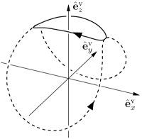
where for example, is the -component of in the vacuum mass basis. As a visual illustration, we show in Fig. 1 the evolution of in the vacuum mass basis for the case of a normal mass hierarchy (solid curve) and for the case of an inverted mass hierarchy with (dashed curve). The trajectory of for each case marks the intersection between the parabolic surface representing
| (76) |
which is equivalent to Eq. (68), and the spherical surface representing
| (77) |
which follows from the fixed magnitude of . The evolution of can be obtained from that of based on Eq. (75).
Of course, the flavor evolution of an initial is described most directly by the -component of in the flavor basis. The unit vectors in this basis are related to those in the vacuum mass basis as
| (78a) | |||||
| (78b) | |||||
| (78c) | |||||
From the above equations and Eq. (75), we obtain
| (79) |
As evolves very little from the initial state for in the case of a normal mass hierarchy and in the case of an inverted mass hierarchy with , there is little flavor evolution in these cases. In contrast, for the case of an inverted mass hierarchy with , we have and , so an initial can be converted essentially fully into a even for .
Taking and ( for ), we show the time evolution of as the solid lines in Figs. 2(a) and 2(b) for a normal and an inverted mass hierarchy, respectively. The cases with the same but ( for ) are shown as the dashed lines. [In order to show the small evolution in the case of a normal mass hierarchy, we have greatly expanded the vertical scale in Fig. 2(a).]
We note that the period of vacuum oscillations in these numerical examples is . This is longer than the bi-polar oscillation periods shown in Fig. 2. In addition, the bi-polar oscillation periods decrease by a factor of 2 when the neutrino density is increased by a factor of 4. These observations can be understood from Eq. (64), even without an outright solution of this equation. In the limit , the second term on the right hand side of Eq. (64b) dominates, and simply rotates around with roughly a constant magnitude and frequency
| (80) |
The average value of in the above equation can be estimated from Eq. (64a):
| (81) |
Combining Eqs. (80) and (81) we obtain
| (82) |
This simple dimensional analysis agrees with the exact expression for the bi-polar period in the normal mass hierarchy case Kostelecky and Samuel (1995). Therefore, for a large neutrino density , the bi-polar oscillation period is much smaller than and decreases as .
IV.2 General Bi-Polar Systems
We next look at a slightly more complicated neutrino-antineutrino system. In particular, we consider a system which is the same as that discussed in Sec. IV.1 except that and have different energies. We again define and as in Eq. (63). Using Eq. (62), we find
| (83a) | |||||
| (83b) | |||||
where
| (84) |
When viewed in the reference frame rotating with angular velocity , the e.o.m. of and derived from Eq. (83) are exactly the same as that in Eq. (64) and must, therefore, have the same solution. When viewed in the lab frame, this NFIS system not only demonstrates the bi-polar oscillation as discussed in Sec. IV.1, but also rotates around at the same time. We regard this kind of flavor transformation as also being of bi-polar type. Note that this bi-polar system has two intrinsic periods, i.e., and . This bimodal feature of the neutrino-antineutrino system was first discussed in Ref. Samuel (1996).
| – | – | – | – | |
|---|---|---|---|---|
| Never | Always | |||
| Always | Never |
Note that the above arguments employing co-rotating frames apply not only to systems consisting of –, but also to systems of –, – or –. Because – systems can develop large flavor mixing in the case of a small mixing angle and an inverted mass hierarchy, the other systems also can exhibit the same phenomenon as long as
| (85) |
where and are the vacuum coupling coefficients of the “spin-up” and “spin-down” NFIS’s, respectively. For convenience, we have listed these conditions in Table 1.
From the simple examples discussed above we can infer a general description of a system possessing bi-polar oscillations: a system composed of two groups of neutrinos and/or antineutrinos of roughly equal numbers, where the corresponding NFIS’s point in two roughly opposite directions and have different characteristic values of .
In Fig. 3 (the solid lines) we illustrate two non-ideal bi-polar systems. These examples consist of gases of initially pure and with and . One of the examples [Fig. 3(a)] illustrates neutrino mixing with a large mixing angle and , and the other [Fig. 3(b)] uses a small mixing angle and .
As the difference between the densities of the two NFIS blocks becomes larger and larger, one of the NFIS blocks will eventually dominate the other, and the system will become synchronized rather than bi-polar. This can been seen from Eq. (83). For simplicity, we work in the frame rotating with angular velocity where the e.o.m. of take the same form as Eq. (64). We note that a key characteristic of any bi-polar system is a configuration in which a large and near constant magnitude vector rotates about [Eq. (64b)]. In this configuration, typically has a small, variable magnitude. If one of the NFIS blocks dominates, it is possible that will be bigger than , and the adiabatic condition can be satisfied. (Note that the rate of change of is bounded by the intrinsic frequency of the bi-polar oscillation.) If the adiabatic condition is satisfied, then will precess rapidly around , with a constant relative angle between them. In this case, will average out to be . At the same time, will have roughly constant magnitude and will rotate around with a angular frequency [Eq. (64a)]
| (86) |
Clearly, the dominant oscillation behavior of the NFIS system is the slow rotation around and the synchronized mode obtains in this case. Indeed, one can explicitly show that is the synchronization frequency of the system in the co-rotating frame.
From the above arguments one can see that the condition for a bi-polar system to degrade into a synchronized mode is the same as that for to adiabatically precess around . Therefore, the criterion for a NFIS system to be bi-polar is that
| (87) |
where is the angle between the directions of and . We note that this criterion is exactly the opposite of the synchronization criterion given in Eq. (54). In many cases, the criterion for bi-polar flavor transformation can be expressed as
| (88) |
We now comment on the stability of the bi-polar mode. Realistic systems of interest usually consist of neutrinos and/or antineutrinos with continuous energy distributions. Because neutrinos (antineutrinos) of different energies have different vacuum oscillation frequencies, one might suspect that the bi-polar mode eventually collapses as a result of destructive interference. We have argued above (Sec. III.2) that the conservation of total effective energy essentially guarantees the stability of the synchronized mode. This conclusion does not extend directly to the bi-polar mode. However, this energy conservation condition does provide some shielding of the two-oppositely-directed-NFIS-block configuration against rapid destructive interference-driven breakdown. This is because the effective energies of the two NFIS blocks ( and ) and the interaction energy of these blocks () sum to almost zero, and because each of these ingredient energies are large in magnitude and not easily altered. If the bi-polar configuration is ever to break down, the two NFIS blocks must disassemble simultaneously in a symmetric way in order to conserve the total effective energy. As a result, the bi-polar mode is at least semi-stable. It has been observed that the two-oppositely-directed-NFIS-block configuration is roughly maintained in example numerical simulations Kostelecky et al. (1993); Kostelecky and Samuel (1994).
IV.3 Bi-Polar Flavor Transformation with a Matter Background
In Fig. 3 we present results of numerical solutions to the e.o.m. for two NFIS blocks [Eq. (31)]. In this figure, we show examples (the dashed and dot-dashed lines) of flavor oscillations in gases of initially pure and in the presence of various matter backgrounds. It can be seen that flavor transformation is suppressed for the scenario with a large mixing angle and a normal mass hierarchy if . On the other hand, large flavor mixing still occurs in these systems with small mixing angles and an inverted mass hierarchy even if the electron density dominates, although the flavor oscillation period is somewhat longer than in the case with no matter background.
This phenomenon can be understood qualitatively by using the concept of co-rotating frames. In the presence of a matter background, the motions of still are governed by Eq. (83) except that is in this case defined as
| (89) |
We decompose into two components: and . These vectors are perpendicular and parallel to , respectively. In the reference frame rotating with angular velocity , we have
| (90a) | |||||
| (90b) | |||||
This configuration is illustrated in Fig. 4. If is very large, will rotate very rapidly and the NFIS’s are not able to follow it. In this limit, will have on average negligible influence on the overall evolution of the system, at least so long as and are not aligned with . Note that this scenario is similar to the simple small mixing angle bi-polar example discussed in Sec. IV.1. However, one difference is that here takes the place of in the simple case. Bi-polar systems with matter backgrounds, therefore, behave similarly to those without.

Consider the simple – system discussed in Sec. IV.1 but now with a large matter background. The two NFIS blocks formed by neutrinos and antineutrinos are initially aligned or anti-aligned with . The field component will perturb the system to break this alignment. The perturbation by is not enough to cause and to deviate much from their original directions. This is because has negligible net effects once the angle between () and is significant. However, the configuration with a misalignment of and relative to is just like the initial configuration of the simple – system discussed in Sec. IV.1. Therefore, for the normal mass hierarchy (), and will oscillate around , and no significant flavor mixing occurs. For the inverted mass hierarchy (), and could completely swap their directions and large flavor mixing will result.
Dynamically, the configuration with aligned with is “stable” because acts as a restoring “force” which prevents from becoming significantly misaligned with it. This is why neutrino-antineutrino gases of initially pure and do not have large flavor mixing if and . On the other hand, the configuration with anti-aligned with is “unstable” because acts as a “force” which drives toward the (“stable”) position of alignment with and then drives it back to the original (“unstable”) position. This is why neutrino-antineutrino gases of initially pure and can have large flavor mixing if and .
V Collective Neutrino Flavor Transformation in Supernovae
To treat neutrino and antineutrino flavor transformation in a core-collapse supernova event, we must account for nonuniformity and anisotropy in the neutrino density distribution. At a radius which is larger than the neutrino sphere radius , the neutrino number density distribution is
| (91) |
where is the neutrino (energy) luminosity, is the normalized neutrino energy distribution, is the average neutrino energy, is the differential solid angle around the radial direction with being the polar angle, and
| (92) |
In general, flavor evolution of neutrinos traveling in different directions above the neutrino sphere will be different due to the anisotropy of the neutrino density distribution. For a qualitative discussion, we will assume the “single-angle approximation” (see, e.g., Ref. Fuller and Qian (2006)) that the flavor evolution history of a radially propagating neutrino is representative of all neutrinos. Under this approximation,
| (93) |
where
| (94a) | ||||
| (94b) | ||||
We will comment on the validity of the single-angle approximation at the end of the section.
When they leave the neutrino sphere, the neutrinos and antineutrinos form two oppositely directed NFIS blocks. For illustrative purposes we assume that and dominate the neutrino species emitted from the proto-neutron star. We will also assume that and have the same luminosity , and that the vacuum coupling coefficients of the two corresponding NFIS blocks are
| (95) |
respectively.
We define a dimensionless quantity
| (96a) | ||||
| (96b) | ||||
| (96c) | ||||
This quantity gives a measure of the inverse of the number density of either neutrino species. Using Eqs. (88), (94b), (95) and (96) we find that the rough boundary condition for supernova neutrinos to transition from the synchronized mode to the bi-polar mode is
| (97) |
where the dimensionless quantity
| (98) |
measures the disparity between the energy spectra of and . If is much smaller than the boundary radius (Bi-polar Starting) of the two collective modes, we can estimate
| (99) |
As neutrinos propagate away from the proto-neutron star, the local neutrino density decreases. Beyond some radius the neutrino density is so low that the collectivity of neutrino flavor transformation breaks down and neutrinos undergo conventional MSW flavor evolution. This occurs if
| (100) |
where is the half-width of the distribution (see the discussion in Sec. III.2). We estimate that
| (101) |
where is the half-width of the () energy spectra. Using Eqs. (94b), (96), (100) and (101) we can obtain a condition for where collectivity of neutrino flavor oscillations will break down:
| (102) |
If is much smaller than the boundary radius where collectivity breaks down, (Bi-polar Ending), we can show that
| (103) |
Taking , , and , we can calculate the boundary radius between the two collective modes and the radius of the boundary separating the collective modes from the regime where conventional MSW evolution dominates. These boundaries are shown in Fig. 5. It is clear that supernova neutrinos are in the synchronized mode near the proto-neutron star (region I in Fig. 5), but could experience bi-polar flavor transformation at a moderate distance (region II). It is only in the region far from the proto-neutron star that neutrinos will undergo conventional MSW transformation (region III). This is very different from the solar neutrino oscillation case, where neutrinos experience only MSW flavor transformation. We note that there are actually no sharp boundaries between these flavor transformation regions. There will be neutrinos and antineutrinos with many different energies in any region above the proto-neutron star. As a result, a particular region in general could host superpositions of various neutrino and antineutrino oscillation modes. Therefore, regions I, II and III should be understood as where synchronized, bi-polar, and conventional MSW type flavor transformations, respectively, dominate.
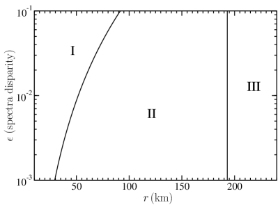
In broad brush, the mixing parameters ( and ), the neutrino and antineutrino energy spectra and luminosities, and and are the principal determinants of the dominant oscillation mode at a particular location. Of course, the actual detailed form of flavor oscillation at any point is also affected by the matter density and electron fraction. For example, if number flux dominates over that for and , neutrinos and antineutrinos in the synchronized mode will evolve as if they were one neutrino with energy [Eq. (60)]. As a result, neutrinos and antineutrinos in this case will experience flavor conversion at radius , where is the MSW resonance radius for a neutrino with energy . This radius is determined by the standard MSW resonance condition,
| (104) |
Governed by the density run in the supernova envelope, neutrinos and antineutrinos may experience the following collective flavor mixing scenarios:
-
•
If the proto-neutron star has a very “thick” envelope, is very large throughout regions I and II and . In this case no significant flavor conversion will occur when neutrinos are in region I. For flavor conversion is also suppressed in region II. For , however, large flavor mixing can occur in region II.
-
•
If the envelope of the proto-neutron star is “thin”, is very small in regions II and III, and . For , almost complete flavor conversion ( and ) occurs around radius in region I. Entering region II, neutrinos and antineutrinos are now dominantly and , and large flavor mixing will occur (see Table 1). For , flavor conversion is suppressed in region I, and large flavor mixing can occur in region II.
-
•
If the proto-neutron star has an envelope of a moderate thickness, is large in region I and part of region II and . In this case, flavor mixing is always suppressed in region I. For , large flavor mixing can occur in region II. The exact flavor oscillation form is not clear for the case in region II. However, some resonance-like behavior around radius could be expected.
The typical collective oscillations described above are idealized. In particular, we have assumed that the gradient of is not so large that the adiabatic condition is violated. If the adiabatic condition is violated, other interesting phenomena may occur. For example, the NFIS’s of neutrinos and antineutrinos may be kicked into a configuration where they are aligned or anti-aligned with at some instant. This corresponds to a maximally mixed state. If this occurs in region I and the adiabatic condition holds from this point on, the NFIS’s will rotate collectively around . This nearly maximal mixing will last until radius or , whichever is smaller. This is the Background Dominant Solution described in Ref. Fuller and Qian (2006).
Our analysis of collective flavor transformation assumed isotropy of the neutrino gases. This is appropriate for the early universe scenario. In the supernova environment the neutrino gas is not isotropic. The anisotropy of the supernova neutrinos has two major effects. One effect is that the neutrinos scattering at some particular point have travelled different distances from the neutrino sphere before they interact. We note that the propagation distances along various trajectories are most different near the neutrino sphere. Close to the proto-neutron star, the electron density is so large that , and breaks the correlation of the NFIS’s on different trajectories. As a result, the NFIS’s on different trajectories develop relative phases. This effect, however, does not compromise our analysis because neutrinos and antineutrinos are essentially kept in their flavor eigenstates by , and the effects of destructive interference are small. After neutrinos propagate away from the proto-neutron star, the distance difference between any two trajectories becomes small.
The other effect of the anisotropy of supernova neutrinos is that the neutrino-neutrino forward scattering potential, and therefore , depends on the angle between the directions of the neutrino momenta [Eq. (28)]. As a result, the effective total NFIS
| (105) |
is different for NFIS’s on different trajectories, and one cannot define a universal total NFIS in the original isotropic sense. However, we note that the NFIS’s on different trajectories are still strongly coupled as a result of large neutrino density. This is why collective neutrino flavor oscillations can arise in the first place. Although the exact neutrino oscillation behavior can only be shown by the numerical simulations which treat the trajectory issue self-consistently, we expect that qualitatively similar flavor oscillations, e.g., large flavor mixing in the and scenario, may occur in the real supernova environment.
VI Conclusions
We have introduced a notation for neutrino flavor isospin which explicitly exhibits symmetry between flavor transformation of neutrinos and antineutrinos. We have pointed out a key quantity in dense gases of neutrinos and/or antineutrinos, the total effective energy, which is conserved in some interesting cases. Using the conservation of the total effective energy, we have proved the stability of synchronized flavor transformation in a simple and intuitive fashion. We have also demonstrated how co-rotating frames can be useful in analyzing collective oscillation in more general cases.
With the concept of total effective energy we have for the first time explained why large flavor mixing occurs for a dense gas of initially pure and with a small mixing angle and an inverted mass hierarchy. We have estimated the oscillation periods of bi-polar systems using simple dimensional analysis. Additionally, we have studied more complicated and more general bi-polar systems by using co-rotating frames. We have also for the first time demonstrated that a dense gas initially consisting of pure and with an inverted mass hierarchy can develop large flavor mixing, even in the presence of a dominant matter background.
We have derived a convenient criterion for determining whether the synchronized or bi-polar type of collective oscillations may arise in a dense neutrino and/or antineutrino gas. Based on this criterion, we have estimated the regions where various modes of flavor oscillation may occur in the supernova environment. We have found that neutrinos emitted from the proto-neutron star in a core-collapse supernova event generally experience synchronized and bi-polar flavor transformations in sequence before the conventional MSW flavor transformation takes over. We have also described the typical flavor oscillation behaviors according to different density runs in the supernova envelope.
Although our analysis of neutrino flavor transformation in the supernova environment is based on crude estimates, it does suggest a picture of neutrino flavor transformations dramatically different from that in the solar case. In particular, because of the large neutrino luminosities, both synchronized and bi-polar types of collective flavor transformations are involved in the supernova scenario.
To go beyond this work we would need to drop a number of the approximations made here and go over to a detailed numerical simulation starting from realistic conditions of neutrino and antineutrino luminosity and spectral distribution. Chief among the requirements of a detailed numerical model would be a self-consistent treatment of flavor evolution on different trajectories from the neutrino sphere. This could be especially important for regions near the neutrino sphere. Even when such detailed numerical simulations are accomplished, the collective behavior of neutrino flavors will remain a complicated phenomenon. This is where our simple physical pictures may be most useful: delineating the expected qualitative behavior of the self-interacting neutrino system in various supernova conditions.
In any case, our results have probably overturned some of the existing paradigms related to the supernova neutrino flavor oscillation problem. Among these, the analyses of future supernova neutrino signals are certainly affected, because most if not all current analyses are based on the assumption that the conventional MSW transformation is valid throughout the supernova environment. Depending how deep the collective large-scale flavor mixing of neutrinos and antineutrinos may occur, the treatment of shock re-heating and nucleosynthesis might also be affected.
Acknowledgements.
This work was supported in part by UC/LANL CARE grant, NSF grant PHY-04-00359, the TSI collaboration’s DOE SciDAC grant at UCSD, and DOE grant DE-FG02-87ER40328 at UMN.References
- Fuller et al. (1987) G. M. Fuller, R. W. Mayle, J. R. Wilson, and D. N. Schramm, Astrophys. J. 322, 795 (1987).
- Fuller et al. (1992) G. M. Fuller, R. W. Mayle, B. S. Meyer, and J. R. Wilson, Astrophys. J. 389, 517 (1992).
- Sigl and Raffelt (1993) G. Sigl and G. Raffelt, Nucl. Phys. B406, 423 (1993).
- Qian et al. (1993) Y.-Z. Qian, G. M. Fuller, G. J. Mathews, R. W. Mayle, J. R. Wilson, and S. E. Woosley, Phys. Rev. Lett. 71, 1965 (1993).
- Qian and Fuller (1995a) Y. Z. Qian and G. M. Fuller, Phys. Rev. D51, 1479 (1995a), eprint astro-ph/9406073.
- Pastor et al. (2002) S. Pastor, G. G. Raffelt, and D. V. Semikoz, Phys. Rev. D65, 053011 (2002), eprint hep-ph/0109035.
- Schirato and Fuller (2002) R. C. Schirato and G. M. Fuller (2002), eprint astro-ph/0205390.
- Balantekin and Yüksel (2005) A. B. Balantekin and H. Yüksel, New J. Phys. 7, 51 (2005), eprint astro-ph/0411159.
- Pantaleone (1992) J. T. Pantaleone, Phys. Rev. D46, 510 (1992).
- Samuel (1993) S. Samuel, Phys. Rev. D48, 1462 (1993).
- Qian and Fuller (1995b) Y.-Z. Qian and G. M. Fuller, Phys. Rev. D52, 656 (1995b), eprint astro-ph/9502080.
- Fogli et al. (2006) G. L. Fogli, E. Lisi, A. Marrone, and A. Palazzo, Prog. Part. Nucl. Phys. 57, 742 (2006), eprint hep-ph/0506083.
- Wolfenstein (1978) L. Wolfenstein, Phys. Rev. D17, 2369 (1978).
- Wolfenstein (1979) L. Wolfenstein, Phys. Rev. D20, 2634 (1979).
- Mikheyev and Smirnov (1985) S. P. Mikheyev and A. Y. Smirnov, Yad. Fiz. 42, 1441 (1985).
- Fuller and Qian (2006) G. M. Fuller and Y.-Z. Qian, Phys. Rev. D73, 023004 (2006), eprint astro-ph/0505240.
- Mikheyev and Smirnov (1986) S. P. Mikheyev and A. Y. Smirnov, in ’86 Massive Neutrinos in Astrophysics and in Particle Physics, edited by O. Frackler and J. Trân Thanh Vân (Editions Frontières, Gif-sur-Yvette, 1986), p. 355.
- Kostelecky and Samuel (1994) V. A. Kostelecky and S. Samuel, Phys. Rev. D49, 1740 (1994).
- Kostelecky and Samuel (1993) V. A. Kostelecky and S. Samuel, Phys. Lett. B318, 127 (1993).
- Kostelecky and Samuel (1995) V. A. Kostelecky and S. Samuel, Phys. Rev. D52, 621 (1995), eprint hep-ph/9506262.
- Samuel (1996) S. Samuel, Phys. Rev. D53, 5382 (1996), eprint hep-ph/9604341.
- Pastor and Raffelt (2002) S. Pastor and G. Raffelt, Phys. Rev. Lett. 89, 191101 (2002), eprint astro-ph/0207281.
- Notzöld and Raffelt (1988) D. Notzöld and G. Raffelt, Nucl. Phys. B307, 924 (1988).
- Kim et al. (1987) C. W. Kim, W. K. Sze, and S. Nussinov, Phys. Rev. D35, 4014 (1987).
- Kim et al. (1988) C. W. Kim, J. Kim, and W. K. Sze, Phys. Rev. D37, 1072 (1988).
- Pantaleone (1998) J. T. Pantaleone, Phys. Rev. D58, 073002 (1998).
- Kostelecky et al. (1993) V. A. Kostelecky, J. T. Pantaleone, and S. Samuel, Phys. Lett. B315, 46 (1993).