STANDING SHOCKS IN TRANS-MAGNETOSONIC ACCRETION FLOWS ONTO A BLACK HOLE

Abstract

Fast and slow magnetosonic shock formation is presented for stationary and axisymmetric magnetohydrodynamical (MHD) accretion flows onto a black hole. The shocked black hole accretion solution must pass through magnetosonic points at some locations outside and inside the shock location. We analyze critical conditions at the magnetosonic points and the shock conditions. Then, we show the restrictions on the flow parameters for strong shocks. We also show that a very hot shocked plasma is obtained for a very high-energy inflow with small number density. Such a MHD shock can appear very close to the event horizon, and can be expected as a source of high-energy emissions. Examples of shocked MHD accretion flows are presented in the Schwarzschild case.

1 Introduction

In connection with the activity of active galactic nuclei (AGNs), compact X-ray sources and inner engines of gamma-ray bursts (GRBs), we consider accreting plasmas onto a black hole. The observed huge energy outputs are mainly originated from the gravitational energy released from infalling matters. When a black hole is rapidly rotating in an external magnetic field, we can also expect the release of the rotational energy of the black hole by the electromagnetic interaction between the black hole’s spin and the magnetic field (see Blandford & Znajek (1977) in the force-free limit; Takahashi et al. (1990), hereafter TNTT90; Hirotani et al. (1992) for ideal MHD flow). The global magnetic field around a black hole should be enhanced by infalling magnetized plasmas, and the magnetic field generated by the dynamo motion of the surrounding plasma can also interact with the spin of the black hole. The “black hole magnetosphere” system is composed of a rotating black hole, surrounding plasmas and magnetic fields, and considered as a central engine of AGN and GRB activities. It would output energy in the form of high-energy radiation (X-rays and $\gamma$-rays) and highly-accelerated plasma outflows (relativistic jets and winds). In both energy output processes, the study of plasma behavior in the magnetosphere is the key to various problems. This situation is very similar to the activity of the solar magnetosphere (i.e., the emission of X-rays and the generation of solar wind). In this paper, we investigate the basic plasma physics of the vicinity very close to a black hole including the magnetosphere.

The magnetosphere is assumed stationary and axisymmetric, and the ideal MHD approximation is assumed. Then, the MHD plasmas stream along magnetic field lines in the magnetosphere, and five field aligned parameters exist; that is, the total energy, total angular momentum, number flux per magnetic flux and entropy of the MHD flow, and the angular velocity of the magnetic field line (see next section). The flows accelerated by gravity pass through magnetosonic points, where the poloidal component of the flow velocity becomes the magnetosonic wave speed. To fall into the black hole, the accreting plasma ejected from the plasma source with low-velocity must pass through the fast and slow magnetosonic points and the Alfvén point, which are singular points in the basic equations. The physical flow solution along a magnetic field line is restricted by the regularity conditions at these singular points (Takahashi, 2002a). That is, the conditions restrict the possible ranges of physical flow parameters.

Hereafter, we will discuss the MHD shock in accretion onto a black hole. Relativistic MHD shocks are discussed by, e.g., Ardavan (1976) and Lichnerowicz (1967, 1976). We apply their formalism to a black hole magnetosphere in Kerr spacetime (for the slow magnetosonic shock, see Takahashi et al. (2002), hereafter TRFT02; Takahashi (2002b); Rilett (2003)). The trans-magnetosonic accretion flow, which is ejected from a plasma source and passes though the first magnetosonic point, results in the shock on the way to the event horizon, and the postshock sub-magnetosonic flow passes through the second magnetosonic point (located inside the shock front) again. Such a MHD shock accretion solution must satisfy the critical conditions at both the first and second magnetosonic points and the shock conditions. Thus, we must adjust the five parameters of the flow to the physically acceptable shocked accretion solution with multiple magnetosonic points by considering both the critical conditions at the magnetosonic points and the jump conditions at the shock front.

In a plausible black hole magnetosphere, global magnetic field lines are generated by the surrounding plasma (e.g., an equatorial disk and its corona). We expect that (1) the magnetic field lines shaped like loops would be distributed around the inner-edge region of the disk, (2) the disk surface and the black hole are connected by the magnetic field lines, where on the disk side of the field lines the footpoints can be anchored to the disk surface at the location of several times the inner-edge radii and on the black hole side the field lines can connect the event horizon from its pole to equator, and (3) the open magnetic field lines connecting the outer region of the disk surface are extended to distant regions (van Putten, 1999; Tomimatsu & Takahashi, 2001; Li, 2002; Uzdensky, 2005). The ingoing (or outgoing) flow is ejected with non-zero velocity from the footpoint on the disk surface, which is a plasma source and is called the “injection point”. Then, along the disk–black hole connecting magnetic field lines, the MHD ingoing flows fall into the black hole, while the outgoing winds would stream along the open magnetic field lines and the loop-like magnetic field lines would enclose static plasmas. (For a high accretion rate accretion disk system, the plasma can fall into the black hole radially from the disk’s inner-edge. In this case, the loop-like configuration of the magnetic field lines would disappear.) By considering the disk–black hole magnetic field lines, non-equatorial accretion flow that falls into the black hole from the high-latitude region is possible. If a MHD shock arises on the non-equatorial inflows and forms a very hot plasma region by the shock, we can expect high-energy emissions in the magnetosphere, which would be distinct from the emissions from the equatorial accretion disk. Such high energy emissions from the hot plasma would directly (or indirectly) carry informations for the strong gravitational field to us.

In our numerical demonstrations for MHD shocked ingoing flows, we should solve the realistic magnetic stream function (Nitta, Takahashi, &Tomimatsu, 1991) for magnetic field lines connecting the disk and black hole. Note that at the shock front magnetic field lines bend toward toroidal and/or poloidal directions. However, in general, it is hard to solve self-consistently the magnetic structure of the magnetosphere. So, for simplicity, without a realistic magnetic stream function, we would only discuss the ingoing trans-magnetosonic flows on a conical magnetic stream function. We assume that at the shock front the magnetic field lines bend only to the toroidal direction. This assumption would be valid near the black hole (at least inside the inner-light surface). Near the injection point, of course, the conical magnetic fields would not be realistic. This is because the conical magnetic field lines do not connect to the equatorial disk surface; that is, we cannot define the footpoints. (Note that we can consider coronal gases distributed above the disk surface as a plasma source. In this case, conical magnetic field may be probable.) Furthermore, in the demonstrations in §4, we only treat the inflow streaming near the equatorial plane. However, we can expect that the qualitative picture is not drastically changed along the magnetic field lines (2) where we leave the equatorial region.

In this paper, we discuss the general relativistic effects on the streaming MHD plasma in the black hole magnetosphere: trans-magnetosonic accretion and MHD shock formation. The accreting flow must be super-magnetosonic at the horizon, and the flow injected from the plasma source with low-velocity must pass through the magnetosonic points (the slow magnetosonic point, the Alfvén point, and fast magnetosonic point). In §2, we present the general relativistic MHD flows. We introduce the field-aligned flow parameters and trans-magnetosonic solutions. The MHD shock formation is studied and the shocked accretion solutions are presented in §3. We explore various types of shocked solutions. The properties of the MHD shock is discussed in §4. We can obtain a very hot plasma region near the event horizon for the MHD shock of a high-energy inflow with small number density, where the energy conversion from the kinetic energy to the magnetic energy is restricted because of the black hole boundary conditions on the toroidal magnetic field. Summary and conclusions are given in §5.

2 Critical Conditions for Trans-Magnetosonic Flows

We consider stationary and axisymmetric ideal MHD accretion flows in Kerr geometry. In Boyer-Lindquist coordinates with the $c=G=1$ unit, the metric of a Kerr black hole is given by

$$ds^{2} = \left(1-\frac{2mr}{\Sigma}\right)dt^{2}+\frac{4amr\sin^{2}\theta}{\Sigma}dtd\phi$$

$$-\frac{A\sin^{2}\theta}{\Sigma}d\phi^{2}-\frac{\Sigma}{\Delta}dr^{2}-\Sigma d\theta^{2}\ ,$$

where $\Delta\equiv r^{2}-2mr+a^{2}$, $\Sigma\equiv r^{2}+a^{2}\cos^{2}\theta$, $A\equiv(r^{2}+a^{2})^{2}-a^{2}\Delta\sin^{2}\theta$, and $m$ and $a$ denote the mass and angular momentum per unit mass of the black hole, respectively. The ideal MHD condition is $u^{\beta}F_{\alpha\beta}=0$, the particle conservation law is $(nu^{\alpha})_{;\alpha}=0$, where $u^{\alpha}$ is the fluid 4-velocity, $n$ is the number density of the plasma, and $F_{\mu\nu}=A_{\nu;\mu}-A_{\mu;\nu}$ is the electromagnetic tensor ($A_{\mu}$ is a vector potential). The equation of motion is $T^{\alpha\beta}_{;\beta}=0$. The energy-momentum tensor is given by

$$T^{\alpha\beta}=\ n\mu u^{\alpha}u^{\beta}-Pg^{\alpha\beta}+\frac{1}{4\pi}\left(F^{\alpha}_{\ \lambda}F^{\lambda\beta}+\frac{1}{4}g^{\alpha\beta}F^{2}\right)\ ,$$ (2)

where $\mu=(\rho+P)/n=m_{\rm part}+(P/n)\Gamma/(\Gamma-1)$ is the relativistic enthalpy, $P$ is the gas pressure, $\rho$ is the total energy density, $\Gamma$ is the adiabatic index, $m_{\rm part}$ is the particle’s mass, and $F^{2}\equiv F_{\mu\nu}F^{\mu\nu}$. The electromagnetic field tensor $F_{\alpha\beta}$ satisfies Maxwell’s equations, ${F^{\alpha\beta}}_{;\beta}=-4\pi j^{\alpha}$ and ${{{}^{\ast}F}^{\alpha\beta}}_{;\beta}=0$, where ${{}^{\ast}F}_{\alpha\beta}\equiv(1/2)\sqrt{-g}\epsilon_{\alpha\beta\gamma\delta}F^{\gamma\delta}$ is the tensor dual to $F_{\alpha\beta}$ and $j^{\alpha}$ is the electric current density. The determinant of the metric is $g$, and $\sqrt{-g}=\Sigma\sin\theta$. We also assume the relativistic polytropic relation $P=K\rho_{0}^{\Gamma}$ (Tooper, 1965), where $\rho_{0}=nm_{\rm part}$ is the rest mass density, which is related to the total energy density by $\rho=\rho_{0}+P/(\Gamma-1)$, and $K$ is a constant along the stream line for an ideal gas. The magnetic and electric fields seen by a distant observer, which are expressed in the Boyer-Lindquist coordinates, are defined by $B_{\alpha}\equiv{{}^{\ast}F_{\alpha\beta}}k^{\beta}$ and $E_{\alpha}=F_{\alpha\beta}k^{\beta}$, where $k^{\alpha}=(1,0,0,0)$ is the time-like Killing vector.

In a stationary and axisymmetric magnetosphere, we can define magnetic field lines as $\Psi(r,\theta)=$ constant lines, where $\Psi(=A_{\phi})$ is the magnetic stream function. The plasma streams along the magnetic field line with five constants of motions (see Camenzind, 1986a): the angular velocity of the field lines, $\Omega_{F}(\Psi)=-F_{tr}/F_{\phi r}=-F_{t\theta}/F_{\phi\theta}$, the particle number flux per unit magnetic flux, $\eta(\Psi)=-nu^{r}G_{t}/B^{r}=-nu^{\theta}G_{t}/B^{\theta}=nu^{t}(\Omega-\Omega_{F})\rho_{w}^{2}/B_{\phi}$, where $G_{t}\equiv g_{tt}+g_{t\phi}\Omega_{F}$ and $\Omega\equiv u^{\phi}/u^{t}$ is the angular velocity of the plasma, the total energy of the magnetized flow, $E(\Psi)=\mu u_{t}-\Omega_{F}B_{\phi}/(4\pi\eta)$, the total angular momentum, $L(\Psi)=-\mu u_{\phi}-B_{\phi}/(4\pi\eta)$, and the entropy $S(\Psi)$, which is related to $K$. Then, we also find the relations $E_{r}=\sqrt{-g}\,\Omega_{F}B^{\theta}/G_{t}$, $E_{\theta}=-\sqrt{-g}\,\Omega_{F}B^{r}/G_{t}$ and $B_{t}=E_{t}=E_{\phi}=0$. From the poloidal components of the equation of motion with five field aligned parameters, we can derive the general relativistic Bernoulli equation (the poloidal equation) (Camenzind, 1986b, 1989, TNTT90) and the general relativistic Grad-Shafranov equation (the trans-field equation) (Camenzind, 1987; Nitta, Takahashi, &Tomimatsu, 1991).

The poloidal equation can be expressed by (see, e.g., TNTT90)

$$\left(\frac{\mu}{\mu_{c}}\right)^{2}(1+u_{p}^{2})=\left(\frac{E}{\mu_{c}}\right)^{2}\left[(\alpha-2M^{2})f^{2}-k\right]\ ,$$ (3)

where $\alpha\equiv g_{tt}+2g_{t\phi}\Omega_{F}+g_{\phi\phi}\Omega_{F}^{2}$, $f\equiv-(G_{\phi}+G_{t}\tilde{L})/[\rho_{w}(M^{2}-\alpha)]$, $k\equiv(g_{\phi\phi}+2g_{t\phi}\tilde{L}+g_{tt}\tilde{L}^{2})/\rho_{w}^{2}$, $G_{\phi}\equiv g_{t\phi}+g_{\phi\phi}\Omega_{F}=g_{\phi\phi}(\Omega_{F}-\omega)$, $\tilde{L}\equiv L/E$ and $\omega\equiv-g_{t\phi}/g_{\phi\phi}$. The relativistic Alfvén Mach number $M$ is defined by

$$M^{2}\equiv\frac{4\pi\mu nu_{p}^{2}}{B_{p}^{2}}=\frac{4\pi\mu\eta u_{p}}{B_{p}}\ ,$$ (4)

where the poloidal component $u_{p}$ of the velocity is defined by $u_{p}^{2}\equiv u^{A}u_{A}$ ($A=r,\theta$), and the poloidal component $B_{p}$ of the magnetic field seen by a distant (lab-frame) observer is defined by $B_{p}^{2}\equiv-B^{A}B_{A}G_{t}^{-2}$. The toroidal component of the magnetic field $B_{\phi}=(\Delta/\Sigma)F_{\theta r}$ can be reduced to $B_{\phi}=-4\pi\eta E\rho_{w}f$, which is expressed in terms of the field-aligned flow’s parameters and the Alfvén Mach number. The denominator of the function $f$ becomes zero when $M^{2}=\alpha$, where the poloidal velocity $|u_{p}|$ equals the relativistic Alfvén wave speed. To obtain the physical MHD flow, which transits from sub-Alfvénic to super-Alfvénic, we must require that the numerator also must be zero. Then, from this regularity condition of the function $f$, we obtain $\tilde{L}=g_{\phi\phi}^{\rm A}(\omega_{\rm A}-\Omega_{F})/G_{t{\rm A}}$ (TNTT90). Note that, for given $\tilde{L}$ and $\Omega_{F}$, we can find one or two radii satisfying the above condition for $\tilde{L}$. We will denote this radius $r=r_{\rm A}$, the “Alfvén radius”, while the point satisfying both $M^{2}=\alpha$ and $r=r_{\rm A}$ is called the “Alfvén point”. The label ‘A’ indicates quantities at the Alfvén radii. Note that, even if $M^{2}\neq\alpha$, the function $f$ can be zero at the Alfvén radius (not the Alfvén point); the toroidal magnetic field $B_{\phi}$ becomes zero, while at the Alfvén point $B_{\phi}$ has a non-zero value. We will denote the zero toroidal field location on a magnetic field line, the “anchor point” (Punsly, 2001). For a streaming MHD plasma, $B_{\phi}$ changes the sign across the anchor point.

In the case of a rotating black hole magnetosphere, there are two light surfaces given by $\alpha=0$: $r=r_{\rm L}^{\rm in}(\Psi)$ and $r=r_{\rm L}^{\rm out}(\Psi)$, where the rotational velocity of the magnetic field line becomes the light velocity as seen by a distant observer. The distribution of light surfaces depends on $\Omega_{F}(\Psi)$, $a$ and $\Psi(r,\theta)$. The inner light surface distributes near the event horizon and encloses it. The plasma source must be located between the inner and outer light surfaces. For a slowly rotating black hole case, $0\leq\omega_{H}<\Omega_{F}$, where $\omega_{H}$ is the angular velocity of the black hole, and for a counter rotating black hole, $\Omega_{F}<0$, two locations of the Alfvén radii are possible along a magnetic field line: $r=r_{\rm A}^{\rm in}(\Psi)$ and $r=r_{\rm A}^{\rm out}(\Psi)$. These radii are always located between the inner and outer light surfaces. Corresponding to two Alfvén radii, we can find two groups of the trans-Alfvénic MHD flow solutions. In one of these the poloidal velocity equals the Alfvén wave speed at the inner Alfvén radii (called the inner Alfvén point), while in the other at the outer Alfvén radii (called the outer Alfvén point). ( Note that these definitions of the inner and outer Alfvén points are slightly different from those in TNTT90.) In these cases, there is the minimum values of ${\tilde{L}}\Omega_{F}$ ($\equiv{\tilde{L}}^{\ast}_{\pm}\Omega_{F}$), for which the Alfvén points exist in the magnetosphere. There, $\tilde{L}={\tilde{L}}^{\ast}_{+}(>0)$ for $\omega_{H}<\Omega_{F}$ and $\tilde{L}={\tilde{L}}^{\ast}_{-}(<0)$ for $\Omega_{F}<0$ satisfy the relation $d{\tilde{L}}/dr_{\rm A}=0$. On the other hand, for a rapidly rotating black hole case $0<\Omega_{F}<\omega_{H}$, the number of the Alfvén point is only one between the two light surfaces for an arbitrary $\tilde{L}$ value. Note that the Alfvén points are located on the light surface when $\tilde{L}\Omega_{F}=1$; this corresponds to the magnetically dominated limit case.

The critical conditions at the fast and slow magnetosonic points are given by the differential form of the poloidal equation (3), which is expressed as :

$$(\ln u_{p})^{\prime}={\cal N}/{\cal D}\ ,$$ (5)

where

$${\cal N} = \left(\frac{E}{\mu}\right)^{2}\left\{\left[{\cal R}(M^{2}-\alpha)C_{\rm sw}^{2}+M^{4}{\cal A}^{2}\right](\ln B_{p})^{\prime}\right.$$ (6)

$$\left.+\frac{1}{2}(1+C_{\rm sw}^{2})\left[M^{4}(M^{2}-\alpha)k^{\prime}-{\cal Q}\alpha^{\prime}\right]\right\}\ ,$$

$${\cal D} = (M^{2}-\alpha)^{2}\left[(C_{\rm sw}^{2}-u_{p}^{2})(M^{2}-\alpha)+(1+u_{p}^{2})M^{4}{\cal A}^{2}{\cal R}^{-1}\right]\$$ (7)

with ${\cal A}^{2}\equiv e^{2}+\alpha k=f^{2}(M^{2}-\alpha)^{2}$, ${\cal R}\equiv\alpha e^{2}-2e^{2}M^{2}-kM^{4}$, ${\cal Q}\equiv\alpha e^{2}-3e^{2}M^{2}-2kM^{4}$, and $e\equiv 1-\tilde{L}\Omega_{F}$. The prime $(^{\prime})$ denotes $\partial_{r}+(B^{\theta}/B^{r})\partial_{\theta}$, which is a derivative along a stream line. The relativistic sound velocity $a_{\rm sw}$ is given by

$$a_{\rm sw}^{2}\equiv\left(\frac{\partial\ln\mu}{\partial\ln n}\right)_{\rm ad}=(\Gamma-1)\frac{\mu-\mu_{c}}{\mu}\ ,$$ (8)

and the sound four-velocity is given by $C_{\rm sw}=a_{\rm sw}/\sqrt{1-a_{\rm sw}^{2}}$.

When the poloidal velocity equals the fast or slow magnetosonic wave speed, the numerator ${\cal D}$ becomes zero. The regularity of the physical solution, to be satisfied by the condition ${\cal N}=0$, is also required at this critical location. The fast and slow magnetosonic points have X-type (saddle-type: physical) or O-type (center-type: unphysical) topology on the integral curves. The condition ${\cal D}={\cal N}=0$ is expressed in terms of four field-aligned conserved quantities. When the values of the three conserved parameters are given at the plasma injection point, the value of the remaining parameter is specified by the critical conditions. Takahashi (2002a) discussed this problem in the Kerr geometry; for example, for given flow parameter sets of $\tilde{L}$, $\Omega_{F}$ and $\zeta_{\rm cr}$, the $\eta$-$r_{\rm cr}$ and $E$-$r_{\rm cr}$ relations were presented, where $\zeta_{\rm cr}\equiv(a_{\rm sw}^{2})_{\rm cr}$ is related to the entropy and the index “cr” means the fast or slow magnetosonic point (to indicate the fast or slow magnetosonic point, we can replace “cr” by “F” or “S”). The fast magnetosonic point can be located between two Alfvén radii, when $(0<){\tilde{L}}^{\ast}_{\pm}\Omega_{F}<{\tilde{L}}\Omega_{F}<{\tilde{L}}^{\rm max/min}_{\pm}\Omega_{F}(<1)$. Here, ${\tilde{L}}^{\rm max/min}_{\pm}$ are defined as $\tilde{L}$ satisfying the relations both $d[\alpha(r_{\rm A})]/dr_{\rm A}=0$ and $\alpha(r_{\rm A})=0$ (where the inner and outer Alfvén radii coincide); ${\tilde{L}}^{\rm max}_{+}$ is used for $\omega<\Omega$ and ${\tilde{L}}^{\rm min}_{-}$ is used for $\Omega_{F}<0$. In this case, the hydro-like accretion solution discussed by Takahashi (2000, 2002a) is possible. We will call such a fast magnetosonic point the middle fast magnetosonic point. The hydro-like solution passes through the outer Alfvén point and the middle fast magnetosonic point, and then falls into the black hole. However, for a rapidly rotating (or counter-rotating) plasma with $|\tilde{L}|>|{\tilde{L}}^{\rm max/min}_{\pm}|$, the hydro-like solution is forbidden and the middle fast magnetosonic point disappears. This is due to the efficient centrifugal barrier on the fluid, so that no solution of ${\cal D}={\cal N}=0$ for the fast magnetosonic point appears between the inner and outer Alfvén points. On the other hand, the magneto-like solution is possible for $\tilde{L}_{\pm}^{\ast}\Omega_{F}<\tilde{L}\Omega_{F}<1$ with the condition $\eta<\eta^{\rm max}$. The magneto-like solution passes through the inner Alfvén point and the inner fast magnetosonic point located between the event horizon and the inner Alfvén point, and then falls into the black hole. In this case, the fluid part of the angular momentum transports to the magnetic part of the angular momentum along the ingoing flow solution. The maximum value $\eta_{\rm max}$ for the inner fast magnetosonic point exists for a hot MHD flow, while $\eta_{\rm max}\to\infty$ in a cold limit. We can expect that the inner fast magnetosonic point disappears for a strong MHD shock with larger $\eta$; such a MHD shocked inflow without the inner fast magnetosonic point is unphysical because the radial velocity of MHD inflow solutions becomes zero at the event horizon, where the number density diverges. The slow magnetosonic points are also obtained from the same regularity condition ${\cal D}={\cal N}=0$. We can find the inner, middle and outer slow magnetosonic points for a suitable $\eta$-value, which are located in the ranges of $r_{\rm L}<r_{\rm S}^{\rm in}<r_{\rm A}^{\rm in}$, $r_{\rm A}^{\rm in}<r_{\rm S}^{\rm mid}<r_{\rm A}^{\rm out}$, $r_{\rm A}^{\rm out}<r_{\rm S}^{\rm out}<r_{\rm L}^{\rm out}$, respectively. For the appearance of the inner or outer slow magnetosonic point, there is the restriction on the $\eta$-value (see Takahashi, 2002a).

In summary, in the case of $\omega_{H}<\Omega_{F}$ or $\Omega_{F}<0$, $\tilde{L}$ must have the value within the range of ${\tilde{L}}^{\ast}_{\pm}\Omega_{F}<\tilde{L}\Omega_{F}<1$ to obtain two possible locations of the Alfvén points in the $u_{p}$-$r$ (or $M^{2}$-$r$) plane. The magneto-like accretion solution is possible when $\eta<\eta^{\rm max}$ and is effective for the magnetically dominated flows. The hydro-like accretion solution is realized when ${\tilde{L}}^{\ast}_{\pm}\Omega_{F}<{\tilde{L}}\Omega_{F}<{\tilde{L}}^{\rm max/min}_{\pm}\Omega_{F}$, and it becomes effective for the hydrodynamically dominated flows. For these two types of solutions, which also depend on $E$, $\eta$ and $S$, the allowable parameter ranges are distinct, so that a discontinuous transition can be expected if the flow parameters change in a secular time-scale. Note that, corresponding to two locations of the Alfvén point, two clearly distinct types of accretion solutions exist; the magneto-like and hydro-like accretion solutions. On the other hand, for a rapidly rotating black hole case, $0<\Omega_{F}<\omega_{H}$, only one Alfvén point exists, so that the distinction between the magneto-like and hydro-like solution is not clear. In the next section, we will only treat the case of $\Omega_{F}>\omega_{H}$ and mainly consider the transition from the hydro-like solution to the magneto-like solution through the standing shock formation.

3 MHD Shock formation in curved spacetime

When we consider the shock formation for accreting MHD flows onto the black hole, we must require a fast (or slow) multiple magnetosonic solution, and must apply the general relativistic MHD shock condition between two fast (or slow) magnetosonic points. As mentioned in the previous section, the critical conditions restrict the allowable ranges of physical flow parameters. In such parameter ranges, we should restrict still more the flow parameter ranges for multiple magnetosonic shocked accretion solutions.

3.1 The jump conditions

Here, we discuss the jump condition for MHD flows in Kerr geometry. The particle number conservation, the energy momentum conservation and the magnetic flux conservation across the shock in a relativistic MHD flow are (Lichnerowicz, 1967, 1976; Appl & Camenzind, 1988)

$$[nu^{\alpha}]^{1}_{2}~{}\ell_{\alpha}=0\ ,$$ (9)

$$[T^{\alpha\beta}]^{1}_{2}~{}\ell_{\alpha}=0\ ,$$ (10)

$$[^{\ast}F^{\alpha\beta}]^{1}_{2}~{}\ell_{\alpha}=0\ ,$$ (11)

where $\ell^{\alpha}$ is the unit vector normal to the shock front, which has only poloidal components for stationary and axisymmetric flows ($\ell^{A}\ell_{A}=-1$). The symbol $[Z]^{1}_{2}\equiv Z_{1}-Z_{2}$ means the change of a certain quantity $Z$ across the shock located at the radius $r=r_{\rm sh}(\Psi)$, where the indeces “1” and “2” mean the properties of the preshock and postshock flows just on the shock front, respectively. From the conditions (9) and (11), the number flux across the shock front $U\equiv nu^{\alpha}\ell_{\alpha}$ and the normal component of the magnetic field (seen by a distant observer) to the shock front $B_{\perp}\equiv B^{\alpha}\ell_{\alpha}$ remain unchanged; that is, $[U]^{1}_{2}=0$ and $[B_{\perp}]^{1}_{2}=0$. We can also obtain $[E_{\parallel}]^{1}_{2}=0$, $[\Omega_{F}]^{1}_{2}=0$ and $[\eta]^{1}_{2}=0$, where $E_{\parallel}\equiv\epsilon_{AB}E^{A}\ell^{B}$ is the tangential component of the electric field $E^{\alpha}$. The quantity $\eta$ can be expressed as $\eta=-UG_{t}/B_{\perp}$. From the condition (10), the following vector remains unchanged across the shock:

$$W^{\alpha}\equiv\mu u^{\alpha}U-\tilde{P}\ell^{\alpha}-\frac{\alpha}{4\pi}\left(\frac{B_{\perp}}{G_{t}}\right)\left(\frac{B^{\alpha}}{G_{t}}\right)\ ,$$ (12)

where $\tilde{P}\equiv P+(B^{2}/8\pi)$ and $B^{2}\equiv(F^{2}/2)=\alpha B_{p}^{2}+B_{\phi}^{2}/\rho_{w}^{2}$ . From the product $W^{\alpha}\ell_{\alpha}$, we obtain the relation

$$[(\mu/n)U^{2}+\tilde{P}]^{1}_{2}=0\ ,$$ (13)

which can be reduced to

$$U^{2}=\frac{\tilde{P}_{2}-\tilde{P}_{1}}{(\mu/n)_{1}-(\mu/n)_{2}}=4\pi\eta^{2}\frac{\tilde{P}_{2}-\tilde{P}_{1}}{M^{2}_{1}-M^{2}_{2}}>0\ .$$ (14)

From the conditions $[W^{t}]^{1}_{2}=0$ and $[W^{\phi}]^{1}_{2}=0$, we also obtain that the constants of motion $E$ and $L$ are continuous across the shock, while entropy $S$, which is the fifth constant of motion, is discontinuous across the shock (see TRFT02). Of course, for the physically realistic shock solution the entropy must increase. Then, we will introduce the entropy related mass flow rate per magnetic flux tube defined by Chakrabarti (1990)

$$\dot{\cal M}\equiv K^{N}\mu_{c}\eta\ ,$$ (15)

where $N=1/(\Gamma-1)$ is the polytropic index. The quantity $\dot{\cal M}$ conserves for a shock-free flow, but it must increase at the shock due to the entropy generation. By using the definitions of the Alfvén Mach number and the relativistic enthalpy, we can express the entropy-related accretion rate as a function of $r$ and $M^{2}$ with the conserved quantities

$$\dot{\cal M}=\frac{M^{2}}{4\pi\mu\eta}\left[\frac{1}{1+N}\left(\frac{\mu}{\mu_{c}}-1\right)\right]^{N}\ ,$$ (16)

where from the poloidal equation the relativistic enthalpy $\mu$ can be expressed as

$$\left(\frac{\mu}{\mu_{c}}\right)^{2}=\left(\frac{E}{\mu_{c}}\right)^{2}\left[(\alpha-2M^{2})f^{2}-k\right]-\left(\frac{B_{p}M^{2}}{4\pi\mu_{c}\eta}\right)^{2}\ .$$ (17)

Thus, we can plot trans-fast MHD solutions as $\dot{\cal M}(r,M^{2})=$ constant ($>0$) curves on the $r$-$M^{2}$ plane. The physically acceptable MHD shock must satisfy the condition $0\leq\dot{\cal M}_{1}<\dot{\cal M}_{2}$ ; $\dot{\cal M}=0$ for a cold flow ($\mu=\mu_{c}$). The flow in the $\dot{\cal M}(r,M^{2})<0$ region is forbidden as a physical solution.

The location of the standing shock front and shock properties depend on the field-aligned flow parameters. To discuss the shock properties, we will introduce the following dimensionless parameters (Appl & Camenzind, 1988, TRFT02):

$$q \equiv \frac{B^{\phi}_{2}}{B^{\phi}_{1}}\ =\ \frac{M^{2}_{1}-\alpha}{M^{2}_{2}-\alpha}\ ,$$ (18)

$$\xi \equiv \frac{n_{2}u^{t}_{2}}{n_{1}u^{t}_{1}}\ =\ \frac{M^{2}_{1}(e-hM^{2}_{2})}{M^{2}_{2}(e-hM^{2}_{1})}q\ ,$$ (19)

where $h\equiv g^{tt}(1-\tilde{L}\omega)$. The parameter $q$ is the ratio of the toroidal magnetic field before to that after the shock, and $\xi$ is the compression ratio; these parameters are quantities seen by a distant observer, and include the gravitational red-shift factor and Lorentz factor for the plasma motion. We also define the plasma frame compression ratio $\lambda$ by

$$\lambda\equiv\frac{n_{2}}{n_{1}}\ =\ \frac{\mu_{2}M^{2}_{1}}{\mu_{1}M^{2}_{2}}\ .$$ (20)

Furthermore, we are interested in the jump of the magnetization rate and temperature of the plasma. The magnetization parameter $\sigma$, which is defined as the ratio of the Poynting flux to the total mass-energy flux seen by a zero angular momentum observer (ZAMO), can be expressed as (TRFT02)

$$\sigma=\frac{B_{\phi}G_{\phi}}{4\pi\eta\mu u^{t}\rho_{w}^{2}}\ =\ -\frac{e-\alpha h}{e-M^{2}h}\ .$$ (21)

The temperature parameter is defined by

$$\Theta\equiv k_{\rm B}T/m_{\rm part}=K\rho_{0}^{1/N}=(\mu/\mu_{c}-1)/(1+N)\ ,$$ (22)

where $T$ is the temperature of the fluid and $k_{\rm B}$ is the Boltzmann constant.

3.2 Shocked accretion solutions

Now, let us consider MHD accretion solutions with a fast/slow magnetosonic shock on the $r$-$M^{2}$ plane. First, we need to find two solutions of the trans-magnetosonic flow (i.e., trans-fast or trans-slow magnetosonic flows corresponding to the fast or slow magnetosonic shock) having the same values of $E$, $L$, $\eta$ and $\Omega_{F}$. By the shock formation, we can connect these two trans-magnetosonic solutions as a multiple magnetosonic accretion solution. Then, the shocked accretion flow passes through the fast or slow magnetosonic points twice. Along each branch of the preshock and postshock solutions, the value of $\dot{\cal M}$ (or the entropy $S$) is different, $\dot{\cal M}_{\rm pre}\neq\dot{\cal M}_{\rm post}$, where the indexes “pre” and “post” indicate the preshock and postshock trans-magnetosonic accretion solution. The values of $\dot{\cal M}_{\rm pre}$ and $\dot{\cal M}_{\rm post}$ are specified by the critical condition at each fast or slow magnetosonic point for the preshock and postshock solutions; that is, $\dot{\cal M}_{\rm pre}=\dot{\cal M}(r_{\rm cr1},M^{2}_{\rm cr1})$ and $\dot{\cal M}_{\rm post}=\dot{\cal M}(r_{\rm cr2},M^{2}_{\rm cr2})$, where the labels ‘cr1’ and ‘cr2’ indicate the first and second fast or slow magnetosonic points, respectively.

When we require a MHD flow solution passing through the slow magnetosonic point S, the Alfvén point A and the fast magnetosonic point F (hereafter “SAF-solution”), from the critical conditions at the fast and slow magnetosonic point, a relation between $E$, $L$, $\eta$ and $\Omega_{F}$ is also specified. So, a change of the value of one of the parameters requires the change of the values of the remaining parameters. In the next section, to demonstrate fast magnetosonic shocked accretion solutions, we will treat the hydro-like SAF-solution as an upstream flow solution and the magneto-like solution as a downstream flow solution for the fast magnetosonic shock formation. When we demonstrate a slow magnetosonic shock formation, we will consider that the downstream flow solution is the magneto-like SAF-solution, while the upstream flow solution is trans-slow magnetosonic solution. Then, we can restrict the values of $\dot{\cal M}_{\rm pre}$ and $\dot{\cal M}_{\rm post}$ for the MHD flow solution passing through the first and second X-type fast magnetosonic (or slow magnetosonic) points, respectively. To find such a SAF-magnetosonic accretion solution, for a given parameter set of $\Omega_{F}$, $E$ and $L$ we can search for the acceptable value of $\eta$ by tuning the regularity conditions (${\cal D}={\cal N}=0$) at both fast and slow magnetosonic points. If a suitable parameter set is obtained, we will find at least two X-type fast/slow magnetosonic points on the $r$-$M^{2}$ plane.

Next, by applying the relativistic jump condition, we can find one (or two) shock location to give $\dot{\cal M}_{2}=\dot{\cal M}_{\rm post}$ with the condition $\dot{\cal M}_{1}=\dot{\cal M}_{\rm pre}$. We will demonstrate an accretion solution with the MHD shock. The accretion solution with a shock is obtained on the $r$-$M^{2}$ plane by plotting $\dot{\cal M}(r,M^{2})=$ constant curves of the two trans-fast magnetosonic (or trans-slow magnetosonic) flow solutions and a vertical line connecting these solution curves at the shock location.

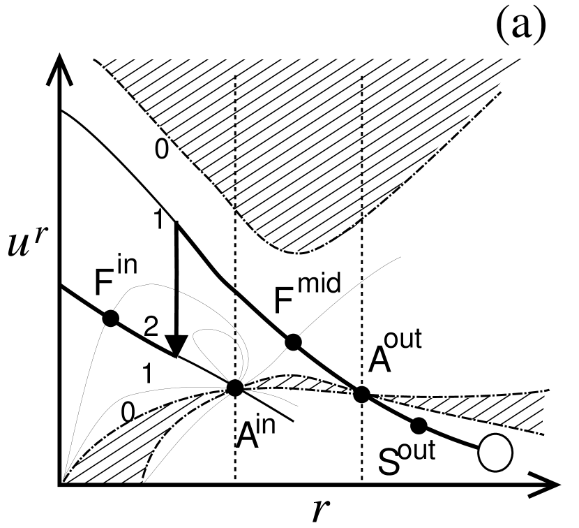
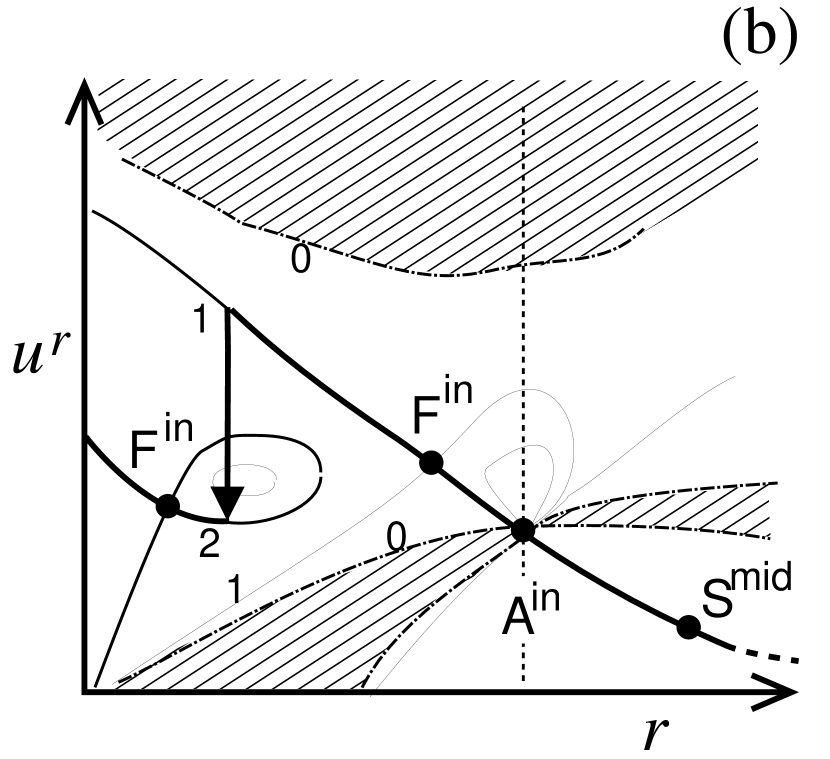
Figure 1: Schematic pictures of physically acceptable accretion solutions with the fast magnetosonic shock (thick curves and arrows). The upstream SAF-solutions are (a) hydro-like and (b) magneto-like, and jump to the downstream trans-fast magnetosonic solution by the shock formation. The large circle in the Left panel (a) represents the plasma source, where the plasma is injected with a finite velocity. In the Right panel (b), the downstream solution does not pass though the inner Alfvén point, but connect to the event horizon with a finite Mach number. The vertical dotted lines are the Alfvén radii. The boundaries of the hatched regions are $\dot{\cal{M}}=0$ curves and are labeled by “0”. The $\dot{\cal{M}}$ value of the downstream curve with the label “2” is grater than that of the upstream with the label “1”; that is, the entropy of the flow is increased by the shock. The other partially plotted thin curves that do not connect the plasma source are unphysical accretion solutions.

Although the numbers (and their locations) of the fast and slow magnetosonic points depend on the flow parameters and the spin of the black hole (Takahashi, 2002a), we can find the following cases of the shocked MHD accretion solutions: two classes of fast magnetosonic shock accretion solutions,

 

FS-i :   inj $\to$ S^out $\to$ A^out $\to$ F^mid $\to$ $<shock>$ $\to$ Fⁱⁿ $\to$ H  .

 

FS-ii :  inj $\to$ S^mid $\to$ Aⁱⁿ $\to$ F${}^{\rm in}_{\rm outer}$ $\to$ $<shock>$ $\to$ F${}^{\rm in}_{\rm inner}$ $\to$ H  ,

and one class of slow magnetosonic shock accretion solution,

 

SS :   inj $\to$ S^out $\to$ $<shock>$ $\to$ S^mid $\to$ Aⁱⁿ $\to$ Fⁱⁿ $\to$ H  .

In Figure 1a (case FS-i), the upstream flow is a hydro-like solution and the downstream postshock flow is a magneto-like solution. The shock formation is possible between these two trans-magnetosonic solutions, where the requirement $\dot{\cal M}_{1}<\dot{\cal M}_{2}$ is satisfied. For the physically acceptable accretion solution, the postshock trans-magnetosonic solution must connect to the event horizon with nonzero four-velocity, $u^{r}_{\rm H}=$ finite. The upstream solution passes through the outer Alfvén point ${\sf A}^{\rm out}$ and the first X-type middle fast magnetosonic point ${\sf F}^{\rm mid}$. After the fast magnetosonic shock, the downstream solution passes through the second X-type inner fast magnetosonic point ${\sf F}^{\rm in}$, and then falls into the black hole H. Figure 1b (case FS-ii) shows that two X-type inner fast magnetosonic points (inner ${\sf F}^{\rm in}$ and outer ${\sf F}^{\rm in}$) locate inside the inner Alfvén point. The upstream magneto-like solution passes through the first X-type inner fast magnetosonic point ${\sf F}^{\rm in}_{\rm outer}$, after passing through the inner Alfvén point ${\sf A}^{\rm in}$. The upstream solution can transit to the downstream trans-fast magnetosonic accretion solution, which passes through the second X-type inner fast magnetosonic point ${\sf F}^{\rm in}_{\rm inner}$ and connect to the event horizon H. On the other hand, in the case of (SS), the upstream solution of the slow magnetosonic shock connects to the outer Alfvén point, but before the Alfvén point the upstream solution can jump to the downstream SAF-solution. This downstream solution passes though the middle slow magnetosonic point ${\sf S}^{\rm mid}$, the inner Alfvén point ${\sf A}^{\rm mid}$ and the inner fast magnetosonic point ${\sf F}^{\rm in}$, and then falls into the black hole.

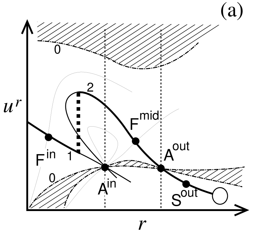
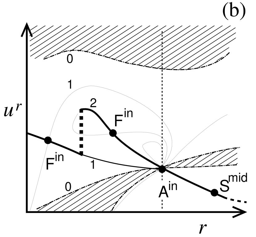
Figure 2: Schematic pictures of unrealistic accretion solutions. The upstream solutions are SAF-solutions, but are broken before the event horizon. In this case, the entropy (or $\dot{\cal{M}}$) of the upstream flow labeled by “2” is grater than that of the downstream labeled by “1”, so that the shock formation is forbidden (thick broken lines mean the disconnection of the upstream and downstream solutions). If the downstream curve is SAF-solution and connects to the plasma source and the event horizon, it is a physical accretion solution without a shock.

One may consider that an upstream accretion solution does not need to connect to the event horizon H. Such a solution is of course unphysical as an accretion solution, but by the shock formation this upstream solution may transit to a downstream physical trans-fast MHD accretion solution that connects to the horizon with a finite (non-zero) four-velocity. Although the upstream SAF-solution has $\dot{\cal M}=\dot{\cal M}_{\rm pre}$ and the downstream trans-fast MHD solution has $\dot{\cal M}=\dot{\cal M}_{\rm post}$, the $\dot{\cal M}=\dot{\cal M}_{\rm pre}$ curve makes a loop or a double-loop on the $r$-$M^{2}$ plane by connecting to the inner Alfvén point (and then it is disconnected to the event horizon) as shown in Figs. 2a and 2b, while the $\dot{\cal M}=\dot{\cal M}_{\rm post}$ curves enclose this loop and one of them connects to H. However, by considering the entropy (or $\dot{\cal M}$) distribution, we conclude that the entropy of the disconnected upstream solution is greater than that of the downstream trans-fast MHD solution; that is, $\dot{\cal M}_{\rm pre}>\dot{\cal M}_{\rm post}$. So the transition from the upstream to downstream solution is forbidden. Thus, for the fast magnetosonic shock formation, both upstream and downstream trans-fast accretion solutions need to connect to the event horizon with non-zero velocity. We should note that even if two trans-magnetosonic accretion solutions exist for a set of values of the field-aligned quantities, no MHD shock may generate under such values. That is, we may find a MHD shock of $\dot{\cal M}_{1}>\dot{\cal M}_{2}$, but such a solution is unphysical.

4 Numerical Results and Discussions

Now we show class (FS-i) fast magnetosonic shock solutions, where a cold ($\Theta\ll 1$) preshock flow is assumed. The solutions are given for the equatorial plane ($\theta=\pi/2$) in the Schwarzschild spacetime ($a=0$). For simplicity, we set the shock normal to the downstream flow; that is, $\ell^{\alpha}=(0,\ell^{r},0,0)$. Then, we obtain the relations $B^{r}_{1}=B^{r}_{2}=B_{\perp}$ and $E^{\theta}_{1}=E^{\theta}_{2}=E_{\parallel}$. Furthermore, without the trans-field equation the poloidal magnetic field is assumed to be the radial configuration denoted by $B^{r}=B_{0}G_{t}/\Sigma$ and $B^{\theta}=0$ ( that is, $\hat{B_{p}}\equiv B_{p}/B_{0}=1/\sqrt{\Delta\Sigma}$) between the plasma source and the event horizon, where $B_{0}=$ constant ($\neq 0$) and the value should be determined at the plasma injection point. Some special radii for the MHD flow are given by the field aligned parameters. The locations of the light surfaces are given by the $\Omega_{F}$ value, and the locations of the Alfvén radii are given by the $\Omega_{F}$ and $\tilde{L}$ values. In addition, setting $\Gamma=4/3$, the values of $\hat{E}\equiv E/\mu_{c}$ and $\hat{\eta}\equiv 4\pi\mu_{c}\eta/B_{0}$ with the values of $\Omega_{F}$ and $\tilde{L}$ determine the locations of the fast and slow magnetosonic points. Then, solution curves $M^{2}=M^{2}(r;\dot{\cal{M}})$ are obtained on the $r$-$M^{2}$ diagram, and the final parameter $\dot{\cal{M}}$ is used to specify an acceptable trans-magnetosonic solution for accretion. ( The solution curves also include an outgoing physically acceptable solution that can take a different value of $\dot{\cal{M}}$ with the accretion solution. The most remaining solution curves are unphysical. )

By assuming a cold preshock flow ($\dot{\cal{M}}_{1}=\dot{\cal{M}}_{\rm pre}=0$), the shock condition (13) can be reduced to

$$\left(\frac{\hat{B_{p}}}{\hat{\eta}}\right)^{2}M^{2}_{1}+\frac{1}{2}\hat{E}^{2}f_{1}^{2}=\left(\frac{\hat{B_{p}}}{\hat{\eta}}\right)^{2}M^{2}_{2}+(\hat{\eta}B_{0}\dot{\cal M}_{2})^{\Gamma-1}\left[\frac{1}{M^{2}_{2}}\left(\frac{\mu_{2}}{\mu_{c}}\right)\right]^{\Gamma}+\frac{1}{2}\hat{E}^{2}f_{2}^{2}\ .$$ (23)

This equation refers to the jump of the Mach number across the shock front. When we obtain the two trans-fast (or trans-slow) magnetosonic solutions $M^{2}=M^{2}_{\rm pre}(r)$ and $M^{2}=M^{2}_{\rm post}(r)$ by tuning both $\hat{E}$ and $\hat{\eta}$ values with the requirement of $\dot{\cal M}_{1}=0$, we can apply the solutions to equation (23); that is, we can set $M^{2}_{1}=M^{2}_{\rm pre}(r_{\rm sh})$ and $M^{2}_{2}=M^{2}_{\rm post}(r_{\rm sh})$. Then, we obtain the location $r=r_{\rm sh}$ satisfying the condition $\dot{\cal{M}}_{2}-\dot{\cal{M}}_{\rm post}=0$. Note that for an acceptable shocked accretion solution we must require the condition $\dot{\cal M}_{2}>\dot{\cal M}_{1}$, while the other field aligned parameters $\Omega_{F}$, $E$, $L$ and $\eta$ are conserved across the shock.

Figure 3: The trans-fast magnetosonic accretion solution with a fast magnetosonic shock (thick black curves); (a) The square of the Alfvén Mach number $M^{2}$ vs. radius $r/m$ and (b) the toroidal component of the magnetic field $\hat{B}_{\phi}$ ($\equiv B_{\phi}/B_{0}$) vs. radius $r/m$ relation are shown with $B_{0}\dot{\cal{M}}=$ constant. After passing through the outer-Alfvén point (A) and the middle-fast magnetosonic point (F^mid), the ingoing flow makes the fast magnetosonic shock near the event horizon. The postshock flow passes through the inner-fast magnetosonic point (Fⁱⁿ), and then falls into the black hole ($r=2m$). The gray curves also show $B_{0}\dot{\cal{M}}=$ constant, but these are unphysical solutions. The flow parameters are given by $\hat{\eta}=0.0108$, $\hat{E}=3.5$, $\tilde{L}/m=4.1$, $m\Omega_{F}=0.14503$, $\Gamma=4/3$, $a=0$ and $\theta=\pi/2$. We obtain $B_{0}\dot{\cal{M}}_{2}=0.05134$ for the postshock flow, while we give $B_{0}\dot{\cal{M}}_{1}=0$ for the preshock flow.

Figure 3a shows the square of the Alfvén Mach number of the shocked accretion solution vs the radial distance. The solution, which passes through the fast magnetosonic points twice, is represented as two $\dot{\cal{M}}=$ constant curves and a vertical arrow (the fast magnetosonic shock). The upstream SAF-curve follows the hydro-like solution, although the slow magnetosonic point is absent on this diagram because of the cold approximation. Then, at the shock location, it transfers to the downstream curve which is the magneto-like solution, and it becomes sub-fast magnetosonic. The shocked flow passes through the fast magnetosonic point again to fall into the black hole. Figure 3b shows the toroidal component of the magnetic field ($\hat{B}_{\phi}\equiv B_{\phi}/B_{0}$) for the shocked solution as a function of radial distance. As the plasma falls inward, the trailed-shape of the magnetic field line ($B_{\phi}<0$) changes to the leading-shaped one ($B_{\phi}>0$) at the Alfvén radius (the anchor point; not the Alfvén point), where $B_{\phi}=0$. The strength of the postshock toroidal magnetic field $|B_{\phi}|$ increases across the fast magnetosonic shock. In Figure 3 the preshock flow solution is plotted as a bold curve starting from the outer light surface with zero-velocity, where the plasma rotates toward the $\phi$-direction with the speed of light. So, a realistic flow should start from a location somewhat inside the outer light surface. In the case of (FS-i), the preshock solution should connect to the plasma source at some location between the outer-Alfvén point and the outer light surface. In Figure 3, gray curves also show $\dot{\cal{M}}=$ constant curves, but they do not pass though the magnetosonic points, or do not connect to the plasma source, except for the upstream $\dot{\cal{M}}=0$ curve of $r_{H}<r<r_{\rm sh}$. Note that the upstream $\dot{\cal{M}}=0$ curve directly connects the plasma source to the event horizon, where the Mach number has a finite value at the event horizon. This curve is also a physically acceptable SAF-solution without the MHD shock. Here, we cannot discuss which of the two accretion solutions; the shocked inflow or the shock-free inflow, is selected as a realistic accretion flow. To answer this question, the stability analysis for shocked MHD flows would be necessary, but that is beyond the scope of our current paper. In the following, we will go ahead to further explore the shocked MHD accretion flows.

Figure 4: The relations between the shock location $r_{\rm sh}/m$ and (a) the energy $\hat{E}$, and (b) particle number flux $\hat{\eta}$ for MHD shocked accretion flows onto a black hole (FS-i solutions). The flow parameters are given by $\tilde{L}/m=4.1$ (thick solid curves) and $4.15$ (thick broken curves), $m\Omega_{F}=0.14503$, $a=0$, and $\theta=\pi/2$. The branch inside the inner Alfvén radius marked by “$\Box$” shows the fast magnetosonic shock, while the branch between the radius marked by “$\bullet$”, which is located inside the middle-fast magnetosonic point, and the inner-Alfvén radius shows the intermediate shock. The curves labeled by “Fp” represent the radii of the inner/middle fast magnetosonic points. The lines labeled by “Ap” represent the radius of the Alfvén point, and the lines with “Ar” indicate the Alfvén radius. The solid and broken lines/curves correspond to $\tilde{L}/m=4.1$ and $4.15$, respectively.

The parameter search for the shocked flow solutions is a standard approach to correctly understand the shock formation in a curved spacetime (TRFT02) and to estimate the activities of a black hole engine. Figure 4a shows the relation between the shock location $r_{\rm sh}$ and the total energy $E$ for the class (FS-i) solutions, which are obtained by solving equation (23) with $\dot{\cal{M}}_{2}-\dot{\cal{M}}_{\rm post}=0$. Figure 4b shows the relation between the shock location $r_{\rm sh}$ and the particle number flux per the magnetic flux $\eta$. The inverse of this quantity exhibits almost the same behavior as $E$. For a physically acceptable shocked MHD accretion solution onto a black hole, the total energy $E$ has the minimum value $E_{\rm min}$ under a certain parameter set of $\Omega_{F}$, $\tilde{L}$ and $a$. It seems that the energy $E$ diverge at $r=r_{\rm sh}^{\rm min}$ (where $\eta E$ has a finite value as seen in Fig. 5), but we stop the calculation at $\hat{E}=100$ (marked by $\circ$). Note that $\hat{E}\to\infty$ (and $\eta\to 0$) with $\tilde{L}\Omega_{F}\to 1$ corresponds to a force-free limit, where the Alfvén radius shifts to the light surface; but in this demonstration $\tilde{L}\Omega_{F}=0.6$; that is, it is not force-free. The possible shock location for physically acceptable shocked accretion flows has the minimum radius $r_{\rm sh}^{\rm min}$ and the maximum radius $r_{\rm sh}^{\rm max}$ (marked by $\bullet$), where these radius are located between the middle- and inner-fast magnetosonic points; that is, $r_{\rm F2}<r_{\rm sh}^{\rm min}$ and $r_{\rm sh}^{\rm max}<r_{\rm F1}$. In Figure 4, the radii of the inner-fast and middle-fast magnetosonic points weakly depend on the value of $E$ or $\eta$. The inner Alfvén radius and the outer Alfvén point are plotted by the vertical lines.

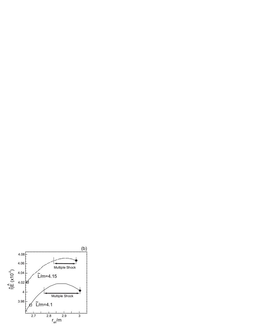
Figure 5: The relations between the shock location $r_{\rm sh}/m$ and the energy flux $\hat{\eta}\hat{E}$ for a (FS-ii) solution. The multiple shock locations are shown in the magnified Right panel (b). The chosen parameter sets are the same as in Fig. 4.

Figure 6: The relations between the shock location $r_{\rm sh}/m$ and the entropy generation $B_{0}\dot{\cal M}_{2}$ by the shock. The chosen parameter sets are the same as in Fig. 4.

Figure 5 shows the value of the total energy flux per magnetic flux tube $\eta E$ at a fast magnetosonic shock location. At a shock location, the value of $\eta E$ for a shocked flow increases with increasing $\tilde{L}$, while the value of $E$ increases and the value of $\eta$ decreases (see Fig. 4). Then, the fast magnetosonic shock with larger energy flux is obtained for the inflow with smaller $E$ (or larger $\eta$) and larger $\tilde{L}$. Figure 6 shows that the relation between the shock location and the entropy related mass flow rate per magnetic flux tube $\dot{\cal M}_{2}$ for the postshock flows. For the shock located near the inner-fast magnetosonic point the lager entropy generation is obtained, while the energy flux becomes small at there. With these flow parameter sets, we may expect a stronger shock formation and/or larger energy release from the hot plasma generated by the shock formation. We will discuss this problem later. Note that a maximum value of $\tilde{L}$ exists for the hydro-like solution; The hydro-like solution is necessary for the middle-fast magnetosonic point to achieve the class (FS-i) solution (Takahashi, 2002a).

When a certain value of the total energy $E$ (or $\eta E$) is given, one or two shock locations are obtained (see Fig. 5b to confirm the multiple-shock locations). When we choose another value of $E$ (or $\eta E$), different values of $\eta$ and $\dot{\cal M}_{2}$ are determined from the critical conditions at the magnetosonic points. The number of physically acceptable shock location depends on the total energy $E$ (or $\eta E$). For example, the number is one for $E_{\ast}\leq E<E_{\rm max}$, and two for $E_{\rm min}\leq E<E_{\ast}$ (a multiple-shock), where $E_{\ast}$ is given at the outermost shock location $r_{\rm sh}^{\rm max}$. When we find the multiple-shock locations for a given parameter set, we should discuss the stability of MHD shocks at each shock location to answer the question of which shock location should be selected as an accretion solution. However, that task is beyond the scope of the present paper. An important point is that the maximum and minimum values (labeled by ‘max’ and ‘min’) exist; that is, the condition for the shock formation is limited by some ranges of the parameter values.

If a shock generates between the inner Alfvén radius and the possible outermost shock radius, which is a segment divided by “$\Box$” and “$\bullet$” in Figs. 4 - 9, the postshock flow becomes sub-Alfvénic. Such a shock is called the “intermediate” magnetosonic shock (the stability of intermediate shocks is discussed by Hada (1994)). In the case of an intermediate shock, the post shocked flow must pass through both inner Alfvén point and inner-fast magnetosonic point. In Figures 4 and 5, we see that the multiple-shock locations are caused in the intermediate shock region. [ For a hot MHD inflow streaming along an area-expanding (diverging) magnetic field line of $B_{p}\propto(1/\sqrt{\Delta\Sigma})r^{-2}$, which is converging along ingoing flows, the possible multiple-shock locations extends to the fast magnetosonic shock region (Goto, 2003). ] For smaller values of $E$ (or larger $\eta E$), multiple-intermediate shock solutions are possible, while an accretion flow with a larger value of $E$ (or smaller $\eta E$) produces a fast magnetosonic shock.

Figure 7: The compression ratio $\lambda$ vs. shock radius relation is shown. The chosen parameter sets are the same as in Fig. 4.

Figure 7 shows the plasma frame compression ratio to be $\lambda<1.7$ for $\tilde{L}/m=4.1$ and $\lambda<1.8$ for $\tilde{L}/m=4.15$; the compression ratio $\xi$ seen by a distant observer is somewhat small because the factor $u^{t}_{2}/u^{t}_{1}<1$ weakens the shock strength. Note that the Lorentz factor $u^{t}$ includes the effects of strong gravity (gravitational red-shift) and the Lorentz boost by the rapid motion of the plasma around the black hole. The strongest shock (the largest $\lambda$ value) is generated around the inner Alfvén radius, where the difference in the Alfvén Mach number between the preshock and postshock trans-fast magnetosonic solutions is also the largest. Although the number density $n_{1}$ of the cold preshock flow is inversely proportional to $M^{2}_{1}$, the function $n_{1}=n_{1}(r)$ has the minimum value around the middle-fast magnetosonic point.

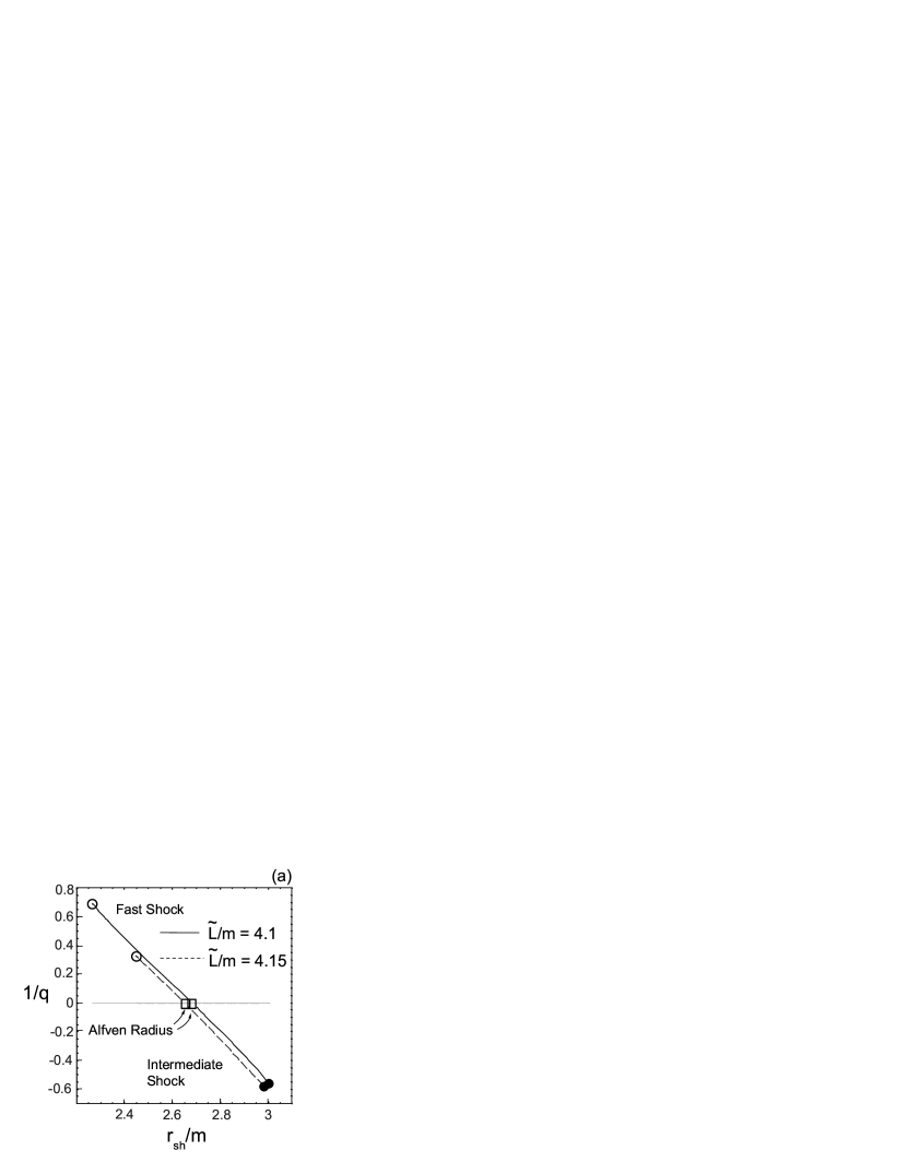
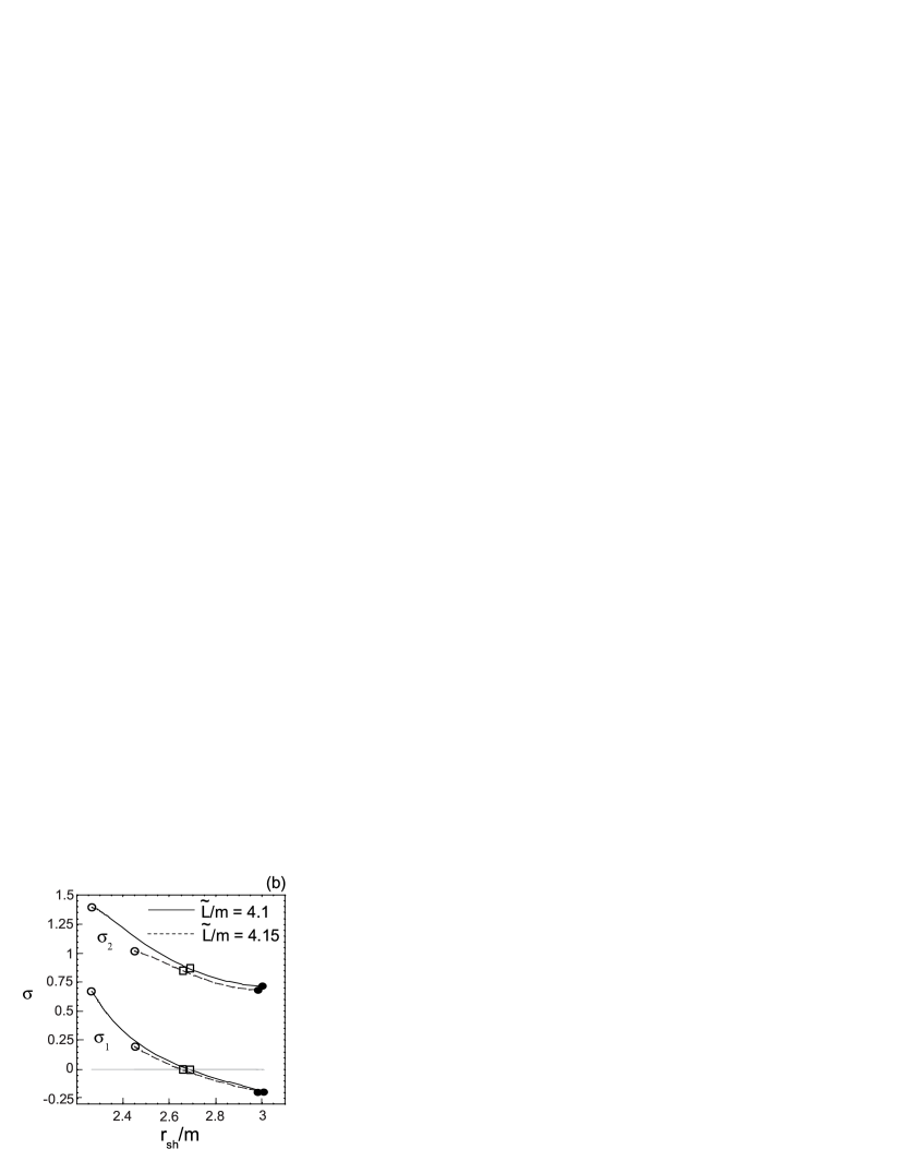
Figure 8: (a) The inverse of the toroidal magnetic field ratio across the shock $1/q$ vs. shock radius relation is shown, while (b) the magnetization parameter $\sigma$ for the pre- and post-shock inflow vs. shock radius relation is shown. The chosen parameter sets are the same as in Fig. 4.

When the shock is generated just on the inner Alfvén radius that is the anchor point for the upstream flow, we see the switch-on shock with $|1/q|=0$ (see Fig.8a), where $(B_{\phi})_{1}=0$ for the preshock flow and $(B_{\phi})_{2}\neq 0$ for the postshock flow. In the fast magnetosonic shock of the class (FS-i), the inner Alfvén radius is not the Alfvén point for the upstream flow solution but it is the Alfvén point for the downstream flow solution. The upstream flow becomes hydrodynamical ($E=\mu u_{t}$, $L=-\mu u_{\phi}$) just on the anchor point. For the positive $q$, as the ratio of the preshock to postshock toroidal magnetic fields $1/q$ increases in magnitude, the magnetization parameter of the postshock flow also increases (see Fig.8b). The property $q>1$ is a characteristic of the fast magnetosonic shock. The negative $q$ corresponds to the intermediate MHD shock, where the sign of the toroidal component of the magnetic field is reversed. In the class (FS-i) solution, the Poynting flux directs inward across the fast magnetosonic shock; that is, the electromagnetic energy is carried to the black hole by the preceding rotation of the anchor point. However, for the intermediate MHD shock, the Poynting fluxes direct outward (inward) for the preshock (postshock) flows; in the intermediate MHD shock the magnetic field line is flipped over at the shock normal.

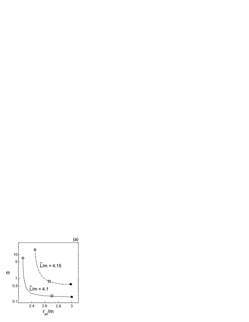
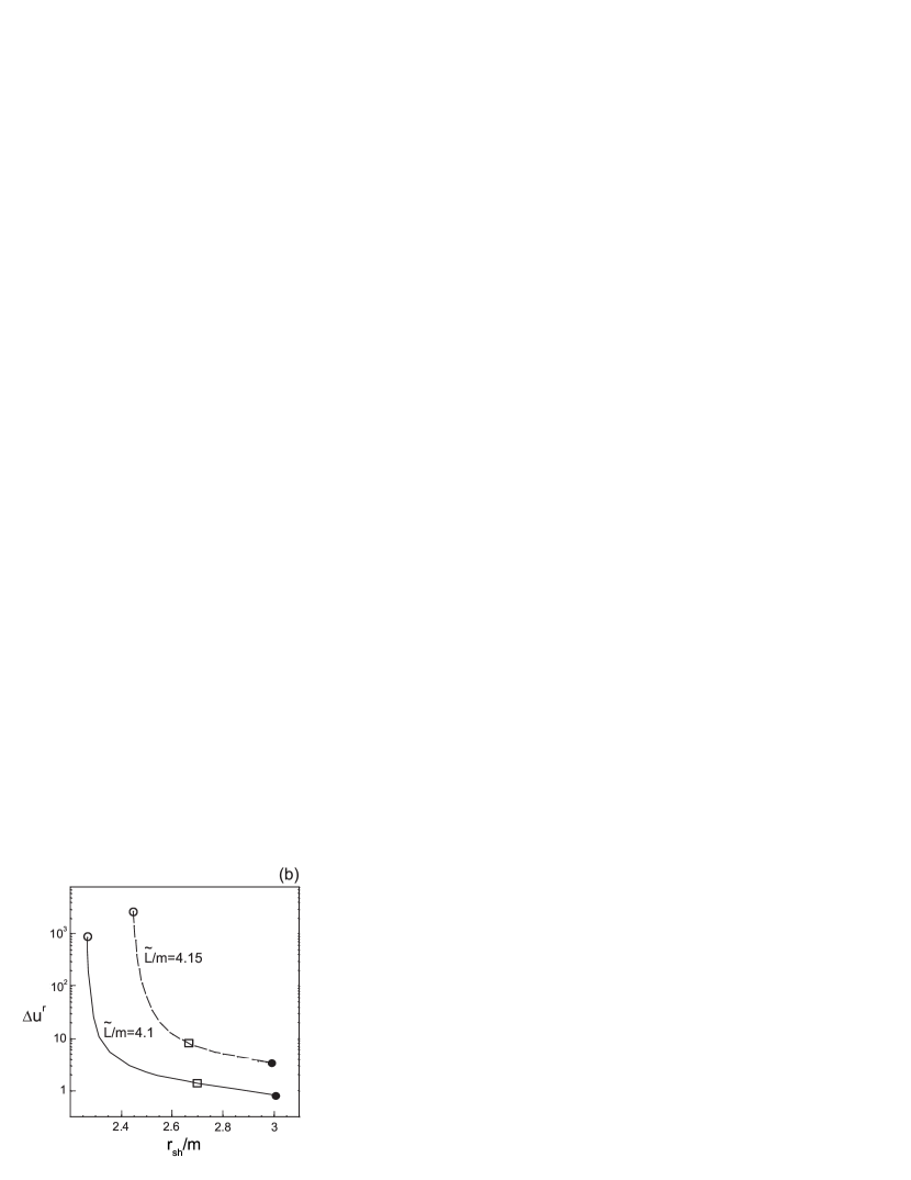
Figure 9: (a) Shows the temperature parameter $\Theta$ vs. shock radius realtion, while (b) shows the jump of the radial four-velocity $\Delta u^{r}$ vs. shock radius relation. The chosen parameter sets are the same as in Fig. 4.

As seen in Fig. 3, when the shock is approaching the inner-fast magnetosonic point, the gap between $M^{2}_{1}$ and $M^{2}_{2}$ becomes small. One may expect that only some fraction of kinetic energy of the preshock flow converts to thermal energy of the postshock flow. In fact, the strength of the shock (the compression ratio $\lambda$) is weakened; this means that the ratio of the preshock and postshock 4-velocities $(u^{r}_{1}/u^{r}_{2})_{\rm sh}$ becomes small. To confirm this, in Figure 9a, the temperature of the postshock flow is shown as a function of the shock radius. Figure 9a (see also Fig. 6), however, indicates that the plasma becomes hotter for the fast magnetosonic shock generated near the inner-fast magnetosonic point. This is because for the shock located near the inner-fast magnetosonic point the plasma’s energy per rest-mass energy $\hat{E}$ is very large and the number flux per magnetic tube $\hat{\eta}$ is small. Furthermore, as seen in Figure 9b that shows the jump of the radial 4-velocity $\Delta u^{r}\equiv(u_{1}^{r})_{\rm sh}-(u_{1}^{r})_{\rm sh}$ at the shock location, the gap $\Delta u^{r}$ becomes large near the inner-fast magnetosonic point even if the ratio $(u^{r}_{1}/u^{r}_{2})_{\rm sh}$ is small (where the value of $\lambda$ has a small value), and a considerable amount of plasma kinetic energy converts to the thermal energy. The plasma kinetic energy, of course, is converted to the magnetic energy by increasing $B_{\phi}$. However, for the fast magnetosonic shock generated near the event horizon, the strength of $(B_{\phi})_{2}$ is $\sim B_{\phi}^{H}~{}[\propto(\omega_{H}-\Omega_{F})B^{r}_{H}]$, which is determined by the boundary condition at the event horizon (see Fig. 3b) and is independent of $u^{r}_{H}$ and $\hat{E}$ (and $\hat{\eta}$). We can say that the toroidal magnetic field $B_{\phi}$ of the stationary shocked accretion flow is restricted by the general relativistic effect (i.e., the hole’s boundary condition), although the information of the horizon cannot propagate to the shock front. Then, the magnetic energy generation cannot dominate in the shock process. Thus, even if the shock is weak, the high temperature postshock inflow is obtained. We can also see that the temperature of the postshock inflow is rising as the shock location approaches the event horizon. So, a cone-like hot plasma column would be built on the event horizon. The high-energy emissions are expected from this hot plasma column with $r_{H}<r<r_{\rm sh}$.

Figure 10: A MHD accretion flow with a slow magnetosonic shock is shown: (a) The square of the Alfvén Mach number and (b) the toroidal magnetic field vs. radius $r/m$ (thick black curves). The preshock curve does not connected to the horizon, but it is physically acceptable through the shock. The flow parameters are given by $\hat{\eta}=0.00521$, $\hat{E}=7.012$, $\tilde{L}/m=4.5$, $m\Omega_{F}=0.14303$, $\Gamma=4/3$, $a=0$ and $\theta=\pi/2$. We obtain $B_{0}\dot{\cal{M}}_{2}=3.591$ for the postshock flow, while we give $B_{0}\dot{\cal{M}}_{1}=0$ for the preshock flow.

Figure 10 shows an accreting flow with the slow magnetosonic shock. Here, the upstream flow solution is cold, so that the injected plasma from a plasma source is super-slow magnetosonic. (Note that the upstream super-slow magnetosonic solution does not necessarily have to pass through the middle-fast magnetosonic point.) After the slow magnetosonic shock, the ingoing flow becomes hot, and passes through the slow magnetosonic point, the Alfvén point and the fast magnetosonic point in this order, and then falls into a black hole. Although, here the slow magnetosonic solution is generated near the outer Alfvén radius, the jump of the Mach number of the slow magnetosonic shock is larger than that of the fast magnetosonic shock (see Fig. 3); that is, the compression ratio becomes higher. The preshock toroidal component of the magnetic field decreases with decreasing radius, and at the slow magnetosonic shock it decreases catastrophically. After the slow magnetosonic shock, the trailed-shape of the magnetic field line changes to the leading one. The detailed properties of the slow magnetosonic shocks are discussed by TRFT02 and Takahashi et al. (in preparation).

5 Summary and Conclusion

We have formulated the MHD shock conditions in Kerr geometry and have discussed MHD accretion flows onto a non-rotating black hole with magnetosonic shock formation. We find that a very hot plasma region can form close to the black hole. To realize these flows, solutions with multiple magnetosonic points are necessary, where the critical conditions at the magnetosonic points are required for the acceptable set of the field-aligned parameters. Furthermore, the MHD shock must be located somewhere between the two magnetosonic points, where the shocked plasma must satisfy the jump conditions. Although the flow parameters should be specified at a plasma injection source (e.g., the surface of an accretion disk or its corona, etc), these parameters for the acceptable MHD accretion flows are specified at some points located near the event horizon by the above conditions. Then, the shocked accretion phenomena would give us information about the plasma sources and the magnetosphere (the inflowing region) in a curved spacetime.

A strong MHD shock with large fluid compression is obtained when the Mach number gap between the preshock and postshock flows is large; such a shock generates around the inner-Alfvén radius. We find that this situation is realized through the transition from the hydro-like preshock flow to the magneto-like postshock flow (type FS-i shocked MHD accretion flow). In the case of a rapidly rotating black hole with $0<\Omega_{F}<\omega_{H}$, this situation with the hydro-like and magneto-like solutions is lost. However, this is possible for the type (FS-ii) shocked MHD accretion flows. In that case, one may not be able to expect strong MHD shock formation with a large compression ratio because the Mach number jump is not so large as in the (FS-i) case. However, a very hot plasma that would be caused by the entropy generation at the shock with $r_{\rm sh}\sim r_{\rm sh}^{\rm min}$ would be expected as in the case of (FS-i) shocked accretion flows.

The Lorentz factor of relativistic jets observed in AGNs is $\sim$ 10 – 100. Therefore, we expect, as an origin of the jet, that the ejected plasma wind from the disk surface has the total energy of $\hat{E}\sim$ 10 – 100. The ejected high-energy plasma streams along the magnetic field lines in the magnetosphere, and forms both outgoing winds and ingoing winds, where the separatrix surface, which separates inflow and outflow regions, depends on the magnetic field distribution in the magnetosphere. Although the outgoing wind outside the separatrix surface is accelerated and would make a relativistic jet, some part of the ejected wind inside the separatrix surface streams toward the black hole because of its strong gravity. Such a wind can produce a MHD shock discussed in this paper. The shocked plasma with $\hat{E}\sim$ 10 – 100 will then make a very hot plasma region. Thus, we can expect that a very hot plasma region is located near the event horizon as a source of high-energy radiation (X- and $\gamma$-ray emissions). Of course, most radiation fluxes would fall into the black hole by the gravitational lens effect, and the energy of the outgoing radiation is lost by the gravitational red-shift effect. However, a huge energy radiation generated by the shock would modify the distributions of the plasma and magnetic field geometry around the black hole. For example, some kind of plasma instabilities or dynamical phenomena, which will include the information on the strong gravity, may be caused by the strong radiation. Such plasma phenomena taking place between the shock and the inner-fast magnetosonic point can propagate outward, and may influence the upstrem flow and further the plasma source. In a magnetized disk–black hole system, “hyperaccretion” onto a slowly rotating black hole is proposed as a model for short gamma-ray bursts (van Putten and Ostriker, 2001). If a very hot plasma region by the MHD shock is generated along the hyperaccretion flow, a fraction of accreting plasma may be blown away as a GRB jet by some plasma instabilities or dynamical phenomena.

When we are interested in a dense accretion flow (with a larger $\eta$ value) that leaves the disk surface without large initial velocity, the expected energy would be $\hat{E}\leq 1$. Although we have explored MHD shocks for larger $\hat{E}$, we also tried to search for the minimum energy of shocked MHD accretion flows (FS-i) under wide ranges of flow parameters (including the variations of $\tilde{L}$, $\Omega_{F}$ and $\theta$ values). However, we did not find a MHD shock solution for $\hat{E}\leq 1$ in our limited parameter search. More systematic analysis will be presented in our subsequent paper (Fukumura et al. in preparation).

In the case of quiet black hole accretion system ($\hat{E}\leq 1$), no MHD shock may be obtained near the equator. However, the MHD shock can be generated along a disk–black hole magnetic field line, and the hot plasma region can form in the high-latitude region of the black hole. Then, we expect that as a signature of AGN activities X- and $\gamma$-ray emissions from the off-equatorial shocked hot plasma are observed directly to us and would be capable of locally illuminating the underlying accretion disk. This could photoionize iron atoms in the disk, causing subsequent iron fluorescence observed in many Seyfert nuclei and Galactic BH candidates. Our MHD shock model thus can be a probable local X-ray radiation source in these systems. Although the estimate of the emergent X-ray spectrum (at the shock) is important, it is beyond the scope of our current investigation.

Appendix A Shock Condition in Plasma Comoving Frame

In this paper, we use the expression with the lab-frame magnetic field $B^{\alpha}$ to analysis the MHD shock conditions. Here, we show the relations between the lab-frame magnetic field and the plasma comoving frame magnetic field.

The magnetic and electric fields in the plasma comoving frame are defined by $b_{\alpha}\equiv{{}^{\ast}F}_{\alpha\beta}u^{\alpha}$ and $e_{\alpha}\equiv F_{\alpha\beta}u^{\beta}$, which satisfy $e_{\alpha}=0$ for the ideal MHD plasma. Then, the homogeneous Maxwell equation can become $(u^{\alpha}b^{\beta}-u^{\beta}b^{\alpha})_{;\alpha}=0$, which means the magnetic flux conservation, and equation (2) becomes

$$T^{\mu\nu}=wu^{\alpha}u^{\beta}-\tilde{P}g^{\alpha\beta}-\frac{1}{4\pi}b^{\alpha}b^{\beta}\ ,$$ (A1)

where $w\equiv n\mu+(b^{2}/4\pi)$, $\tilde{P}\equiv P+(b^{2}/8\pi)$ and $b^{2}\equiv-b^{\alpha}b_{\alpha}$. The lab-field $B^{\alpha}$ denoted in the Boyer-Lindquist coordinates are related to the comoving magnetic field $b^{\alpha}$ by

$$B_{r} = \sqrt{-g}F^{\phi\theta}\ =\ G_{t}b_{r}/\hat{e}\ ,$$ (A2)

$$B_{\theta} = \sqrt{-g}F^{r\phi}\ =\ G_{t}b_{\theta}/\hat{e}\ ,$$ (A3)

$$B_{\phi} = \sqrt{-g}F^{\theta r}\ =\ (G_{t}b_{\phi}-G_{\phi}b_{t})/\hat{e}\ ,$$ (A4)

where $\hat{e}\equiv(E-\Omega_{F}L)/\mu$. From the shock conditions, the following scalar $U$ and two vectors remain unchanged across the shock (Lichnerowicz, 1967) :

$$U \equiv nu_{\perp}\ ,$$ (A5)

$$V^{\alpha} \equiv b_{\perp}u^{\alpha}-u_{\perp}b^{\alpha}\ ,$$ (A6)

$$W^{\alpha} \equiv u_{\perp}wu^{\alpha}-\tilde{P}\ell^{\alpha}-(1/4\pi)b_{\perp}b^{\alpha}\ ,$$ (A7)

where $u_{\perp}\equiv u^{\alpha}\ell_{\alpha}$ and $b_{\perp}\equiv b^{\alpha}\ell_{\alpha}$ (the index “$\perp$” indicates the normal component of the vector to the shock front). Note that $V^{\alpha}\ell_{\alpha}=0$. Furthermore, from the product $V^{\alpha}W_{\alpha}$ we obtain the relation $[\mu b_{\perp}]^{1}_{2}=0$, which is equivalent to $[B_{\perp}]^{1}_{2}=0$, where $B_{\perp}\equiv B^{\alpha}\ell_{\alpha}$. Thus, the qantity $B_{\perp}$ ( or $\mu b_{\perp}$) in a curved-space is a shock invariant. Note that the normal component of the comoving-frame magnetic field changes across the shock, while in the non-relativistic limit we find $\mu=\mu_{c}=m_{\rm part}$, so that $b_{\perp}$ remains unchanged.

References

- Ardavan (1976) Ardavan, H. 1976, ApJ, 206, 822
- Appl & Camenzind (1988) Appl, S.,& Camenzind, M. 1988, A&A, 206, 258
- Blandford & Znajek (1977) Blandford, R. D., & Znajek, R. L. 1977, MNRAS, 179, 433
- Camenzind (1986a) Camenzind, M. 1986a, A&A, 156, 137
- Camenzind (1986b) Camenzind, M. 1986b, A&A, 162, 32
- Camenzind (1987) Camenzind, M. 1987, A&A, 184, 341
- Camenzind (1989) Camenzind, M. 1989, in Accretion Disks and Magnetic Fields in Astrophysics, ed. G. Belvedere (Dordrecht:Kluwer), 129
- Chakrabarti (1990) Chakrabarti, S. K. 1990, MNRAS, 246, 134
- Goto (2003) Goto, J. 2003, Master thesis, Aichi Univ. of Education
- Hada (1994) Hada, T. 1994, Geophys. Res. Lett., 21, 2275
- Hirotani et al. (1992) Hirotani, K., Takahashi, M., Nitta, S., & Tomimatsu, A. 1992, ApJ, 386, 455
- Li (2002) Li, L. -X 2002, ApJ, 567,463
- Lichnerowicz (1967) Lichnerowicz, A. 1967, Relativistic Hydrodynamics and Magnetohydrodynamics (New York : Benjamin Press)
- Lichnerowicz (1976) Lichnerowicz, A. 1976, J. Math. Phys. 17, 2135
- Nitta, Takahashi, &Tomimatsu (1991) Nitta, S., Takahashi, M., & Tomimatsu, A. 1991, Phys. Rev. D, 44, 2295
- Punsly (2001) Punsly, B. 2001, Black Hole Gravitohydromagnetics (Springer)
- Rilett (2003) Rilett, D. 2003, Ph. D. thesis, Montana State Univ.
- Takahashi et al. (1990) Takahashi, M., Nitta, S., Tatematsu, Y., & Tomimatsu, A. 1990, ApJ, 363, 206 (TNTT90)
- Takahashi (2000) Takahashi, M. 2000, in Proceedings of the 19th Texas Symposium on Relativistic Astrophysics and Cosmology, ed. E. Aubourg, T. Montmerle, L. Paul & P. Peter (North-Holland, Amsterdam) CD-ROM 01/27.
- Takahashi (2002a) Takahashi, M. 2002a, ApJ, 570, 264
- Takahashi (2002b) Takahashi, M. 2002b, in Proceedings of the 8th Asian-Pacific Regional Meeting (vol.II), eds. S. Ikeuchi et al. (Tokyo:PASJ), 359
- Takahashi et al. (2002) Takahashi, M., Rilett, D., Fukumura, K., & Tsuruta, S. 2002, ApJ, 572, 950 (TRFT02)
- Tomimatsu & Takahashi (2001) Tomimatsu, A., & Takahashi, M. 2001, ApJ, 552, 710
- Tooper (1965) Tooper, R. F. 1965, ApJ, 142, 154
- Uzdensky (2005) Uzdensky, D. A. 2005, ApJ, 620, 889
- van Putten (1999) von Putten, M. H. P. M. 1999, science, 284, 115
- van Putten and Ostriker (2001) von Putten, M. H. P. M. & Ostriker, E., C. 2001, ApJ, 552, L31