The OSER project

Abstract

The OSER project (Optical Scintillation by Extraterrestrial Refractors) is proposed to search for scintillation of extragalactic sources through the galactic – disk or halo – transparent $\mathrm{H_{2}}$ clouds, the last unknown baryonic structures. This project should allow one to detect column density stochastic variations in cool Galactic molecular clouds of order of $\sim 3\times 10^{-5}\,\mathrm{g/cm^{2}}$ per $\sim 10\,000\,\mathrm{km}$ transverse distance.

1 The transparent baryonic matter and its possible signature

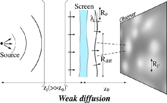
Considering the results of baryonic compact massive objects searches (Lasserre et al. [2000]; [Afonso et al. 2003]; [Alcock et al. 2000]), cool molecular hydrogen ($\mathrm{H_{2}}$) clouds should now be seriously considered as a possible major component of the Galactic baryonic hidden matter. It has been suggested that a hierarchical structure of cold $\mathrm{H_{2}}$ could fill the Galactic thick disk ([Pfenniger & Combes 1994]) or halo ([De Paolis et al. 1995]), providing a solution for the Galactic hidden matter problem. This gas should form transparent “clumpuscules” of $10\,\mathrm{AU}$ size, with a column density of $10^{24-25}\,\mathrm{cm^{-2}}$, and a surface filling factor smaller than 1%. Refraction through such an inhomogeneous transparent $\mathrm{H_{2}}$ cloud (hereafter called screen) distorts the wave-front of incident electromagnetic waves (Fig. 1, see [Moniez 2003] for details). The extra optical path induced by a screen at distance $z_{0}$ can be described by a function $\delta(x_{1},y_{1})$ in the plane transverse to the observer-source line. The amplitude in the observer’s plane after propagation is described by the Huygens-Fresnel diffraction theory:

$$A_{0}(x_{0},y_{0})=\frac{Ae^{2i\pi z_{0}/\lambda}}{2i\pi R_{F}^{2}}\times\int\!\!\int_{-\infty}^{+\infty}e^{\frac{2i\pi\delta(x_{1},y_{1})}{\lambda}}e^{i\frac{(x_{0}-x_{1})^{2}+(y_{0}-y_{1})^{2}}{2R_{F}^{2}}}dx_{1}dy_{1},$$ (1)

where $A$ is the incident amplitude (before the screen), taken as a constant for a very distant on-axis point-source, and $R_{F}=\sqrt{\lambda z_{0}/2\pi}$ is the Fresnel radius. $R_{F}$ is of order of $1500\,\mathrm{km}$ to $15\,000\,\mathrm{km}$ at $\lambda=500\,\mathrm{nm}$, for a screen distance $1\,\mathrm{kpc}<z_{0}<100\,\mathrm{kpc}$. $R_{F}$ characterizes the $(x_{1},y_{1})$ domain that contributes significantly to the integral (a few Fresnel radii). For a point-like source, the intensity in the observer’s plane shows interferences (speckle) if $\delta(x_{1},y_{1})$ varies stochastically of order of $\lambda$ within the Fresnel radius domain. This variation rate is comparable to the average gradient that characterizes the hypothetic $\mathrm{H_{2}}$ structures.

Figure 1: The two scintillation regimes (see text): $R_{diff}\gg R_{F}$ (left), $R_{diff}<R_{F}$ (right).

As for radio-astronomy ([Lyne & Smith 1990]), the stochastic variations of $\delta(x_{1},y_{1})$ are characterized by the diffusion radius $R_{diff}$, defined as the transverse separation for which the root mean square of the optical path difference is $\lambda/2\pi$.
- If $R_{diff}\gg R_{F}$, the screen is weakly diffusive and moderately distorts the wavefront, producing low contrast patterns with length scale $R_{F}$ in the observer’s plane (Fig. 1 left).
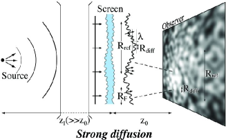
- If $R_{diff}<R_{F}$, the screen is strongly diffusive; two modes occur, the diffractive scintillation – producing strongly contrasted patterns characterized by the length scale $R_{diff}$ – and the refractive scintillation – giving less contrasted patterns and characterized by the large scale structures of the screen $R_{ref}$ – (Fig. 1 right).
Basic configurations: Fig. 2 (left and center) displays the expected intensity variations in the observer’s plane for a point-like monochromatic source observed through a transparent screen with a step of optical path $\delta=\lambda/4$ and through a prism edge. The inter-fringe is $\sqrt{\pi}R_{F}$, the unique distance scale here.

Figure 2: diffraction patterns in the observer’s plane (see text). The $X_{0}-\mathrm{axis}$ ($X_{0}=x_{0}/\sqrt{\pi}R_{F}$) is perpendicular to the structure’s edge. The origin is the intercept of the source-step line with the observer’s plane.

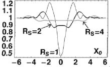
2 Limitations from spatial and temporal coherences

At optical wavelengths, the diffraction pattern contrast is severely limited by the size of the incoherent source $r_{s}$. Fig. 2 (right) shows the diffraction patterns for various reduced source radii, defined as $R_{S}=r_{s}/(\sqrt{\pi}R_{F})\times z_{0}/z_{1}$, where $z_{1}$ is the distance from the source to the screen. In return, temporal coherence with the standard UBVRI filters is sufficiently high to enable the formation of contrasted interferences in the configurations considered here.

3 What is to see?

An interference pattern with inter-fringe of $\sim R_{F}$ ($1000-10\,000\,\mathrm{km}$ at $\lambda=500\,\mathrm{nm}$) is expected to sweep across the Earth when the line of sight of a sufficiently small astrophysical source crosses an inhomogeneous transparent Galactic structure (Table 1). This pattern moves at the relative transverse velocity $V_{T}$ of the screen. In the present paper, we assume that the scintillation is mainly due to pattern motion rather than pattern instability (frozen screen hypothesis), as it is usually the case in radioastronomy observations ([Lyne & Smith 1990]). At the distance of the Galactic $\mathrm{H_{2}}$ clouds we are interested in, we expect a typical modulation index $m_{scint}$ (or contrast) ranging between 1% and $\sim 20\%$ at $\lambda=500nm$, critically depending on the source apparent size; the time scale $t_{scint}=R_{F}/V_{T}$ of the intensity variations is of order of a minute. As the inter-fringe scales with $\sqrt{\lambda}$, one expects a significant difference in the time scale $t_{scint}$ between the red side of the optical spectrum and the blue side. This property might be used to sign the diffraction phenomenon at the $R_{F}$ natural scale.

Table 1: Configurations leading to strong diffractive scintillation assuming $R_{diff}\leq R_{F}$. Numbers are given for $\lambda=500\,\mathrm{nm}$.

		SCREEN
		atmos-	solar	solar	Galactic
		phere	system	suburbs	thin disk	thick disk	halo
Distance		$10\,\mathrm{km}$	$1\,\mathrm{AU}$	$10\,\mathrm{pc}$	$300\,\mathrm{pc}$	$1\,\mathrm{kpc}$	$10\,\mathrm{kpc}$
$R_{F}$ to $\times$ by $\left[\frac{\lambda}{500\,\mathrm{nm}}\right]^{\frac{1}{2}}$		$2.8\,\mathrm{cm}$	$109\,\mathrm{m}$	$157\,\mathrm{km}$	$860\,\mathrm{km}$	$1570\,\mathrm{km}$	$5000\,\mathrm{km}$
Transverse speed $V_{T}$		$1\,\mathrm{m/s}$	$10\,\mathrm{km/s}$	$20\,\mathrm{km/s}$	$30\,\mathrm{km/s}$	$40\,\mathrm{km/s}$	$200\,\mathrm{km/s}$
$t_{scint}$ to $\times\left[\frac{\lambda}{500\,\mathrm{nm}}\right]^{\frac{1}{2}}\left[\frac{R_{diff}}{R_{F}}\right]$		$0.03\,\mathrm{s}$	$0.01\,\mathrm{s}$	$8\,\mathrm{s}$	$29\,\mathrm{s}$	$40\,\mathrm{s}$	$25\,\mathrm{s}$
Optical depth $\tau_{scint}$		$1$			total $>10^{-7}$
$m_{scint}$ in % to multiply by			$32\%\times$	$2.2\%\times$	$4.1\%\times$	$2.2\%\times$	$7.1\%\times$
$\left[\frac{\lambda}{500\,\mathrm{nm}}\right]^{\frac{1}{2}}\left[\frac{R_{diff}}{R_{F}}\right]\left[\frac{r_{s}}{r_{\odot}}\right]^{-1}$		$100\%$	$\left[\frac{d}{10\mathrm{pc}}\right]$	$\left[\frac{d}{1\mathrm{kpc}}\right]$	$\left[\frac{d}{10\mathrm{kpc}}\right]$	$\left[\frac{d}{10\mathrm{kpc}}\right]$	$\left[\frac{d}{100\mathrm{kpc}}\right]$
SOURCE		DIFFRACTIVE MODULATION INDEX $m_{scint}$
Location	Type	(to multiply by $\sqrt{\lambda/500\,\mathrm{nm}}\times R_{diff}/R_{F}$)
nearby 10pc	any star	$\ll 1\%$	$<100\%$
Galactic 8kpc	star	in a	100%	1-70%	1-10%
LMC 55kpc	A5V ($r_{s}=1.7r_{\odot}$)	tele-	100%	70%	13%	7%	2%
M31 725kpc	B0V ($r_{s}=7.4r_{\odot}$)	scope	100%	100%	40%	22%	7%
z=0.2–0.9Gpc	SNIa	$>1\,\mathrm{m}$	100%	70%	13%	7%	2%
z=1.7–1.7Gpc	Q2237+0305		100%	$>45\%$	$>8\%$	$>4\%$	$>1.4\%$

4 Feasibility studies: simulation

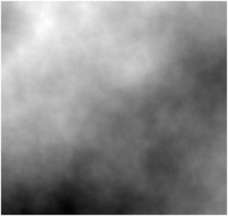
We have simulated the phase delay function $\Phi(x_{1},y_{1})=2\pi\delta(x_{1},y_{1})/\lambda$ of a fractal cloud, described by the Kolmogorov turbulence law (Fig. 3 left). We calculated the diffraction image of a point-like source on Earth (Fig. 3 up-right) from the Fast Fourier Transform of function $exp\left[i\Phi(x_{1},y_{1})+i\frac{x_{1}^{2}+y_{1}^{2}}{2R_{F}^{2}}\right].$ The illumination on Earth due to an extended incoherent source is then obtained by integrating the intensities due to each elementary source.

Figure 3: Phase delay $\Phi(x_{1},y_{1})$ after crossing a turbulent cloud (left); Illumination from a point source (up right); Illumination from a A5V-LMC star versus time (down right).

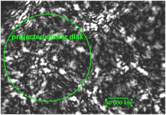
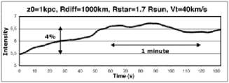
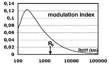
This is equivalent to integrate the intensity image of a point source within the projected source stellar-disk of radius $r_{s}\times z_{0}/z_{1}$. The expected light-curve from a A5V LMC star, as seen through a cloud located at 1kpc, with $R_{diff}=1000km$ and transverse speed $V_{T}=40km/s$, is given in Fig. 3 down-right. Using this simulation, we have been able to estimate the modulation index as a function of the crucial parameter $R_{diff}$ (Fig. 4).

Figure 4: Modulation index of the intensity from a A5V LMC star, as seen through a Galactic molecular cloud located at 1kpc as a function of $R_{diff}$.

5 Toward an experimental setup

Table 1 shows that the search for diffractive scintillation induced by a Galactic molecular cloud needs the capability to sample every $\sim 10\,\mathrm{s}$ (or faster) the luminosity of stars with $M_{V}>20$ (A5V star in LMC or B0V in M31 –or smaller–), with a precision of $\sim 1\%$. This performance can be achieved using a telescope diameter larger than two meters, with a high quantum efficiency detector allowing a negligible dead-time between exposures (like frame-transfer CCDs). Multi-wavelength detection capability is highly desirable to exploit the dependence of the diffractive scintillation pattern with the wavelength.

The $1\%$ surface filling factor predicted if the galactic dark matter is completely made of gaseous structures is the maximum optical depth $\tau_{scint}^{max}$ for all the possible scintillation regimes. Let $\alpha$ be the fraction of halo made of such gaseous objects; under the pessimistic hypothesis that strong diffractive regime occurs only when a gaseous structure enters or leaves the line of sight, the duration for this regime is $\sim 5$ minutes (time to cross a few fringes) over a total crossing time of $\sim 400$ days. Then the diffractive regime optical depth should be at least $\tau_{scint}^{min}\sim 10^{-7}\alpha$ and the average exposure needed to observe one event of $\sim 5$ minute duration is $10^{6}/\alpha\,\mathrm{star\times hr}$ . At isophot $M_{V}=23mag/arcsec^{2}$ of LMC, SMC or M31, about $10^{5}$ stars per square degree with $20<M_{V}<21$ –i.e. small enough– can be monitored ([Elson et al. 1997]; [Hardy 1978]). It follows that a wide field detector is necessary to monitor enough small stars.

6 Foreground effects, background to the signal

Atmospheric effects: Surprisingly, atmospheric intensity scintillation is negligible through a large telescope ($m_{scint}\ll 1\%$ for a $>1\,$m diameter telescope ([Dravins et al. 1997-98])). Any other long time scale atmospheric effect such as absorption variations at the sub-minute scale (due to cirruses for example) should be easy to recognize as long as nearby stars are monitored together.
The solar neighbourhood: Overdensities at $10\,\mathrm{pc}$ could produce a signal very similar to the one expected from the Galactic clouds. In such a case, even big stars would undergo a strong diffractive scintillation, contrary to the expectation from more distant screens; simultaneous monitoring of various types of stars should allow one to discriminate effects due to nearby gas or to remote gaseous structures.
Sources of background? Asterosismology, granularity of the stellar surface, spots or eruptions produce variations of different amplitudes and time scales. A rare type of recurrent variable stars exhibit emission variations at the minute time scale ([Sterken & Jaschek 1996]), but they are easy to identify from spectrum.

7 Preliminary studies with the NTT

Two nights of observations with the NTT were attributed for testing the concept of scintillation in june 2004. We monitored stars located behind or on the edge of Bok globules, searching for scintillation signal due to the gas. We got 5400 exposures of $T_{exp}=7s$ taken with the infra-red SOFI detector, the only one operating with a short readout time (5.5s). The K-band is not optimal for our purpose, but allows to detect stars through the dusty Bok clouds. Unfortunately, only 948 measurements had a seeing smaller than 1.5 arcsec towards B68 globule. We produced the light curves of 2873 stars using the EROS software. After selection and identification of known artifacts (hot pixels, dead zones, bright egrets…), we found only four stars with significant variability, all of four interestingly located near the Bok globule limit. As these limits are natural places for discontinuities, there is a strong interest to clarify and confirm the status of these stars with better quality data. Nevertheless, we can already conclude that the signal we are searching for should not be overwhelmed by background.

8 Conclusions and perspectives

The opportunity to search for scintillation results from the subtle coincidence between the arm-lever of interference patterns due to hypothetic diffusive objects in the Milky-Way and the size of the extra-galactic stars. The hardware and software techniques required for such searches are available just now. If a signal is found, one will have to consider an ambitious project involving synchronized telescopes, a few thousand kilometers apart. Such a project would allow to temporally and spatially sample an interference pattern, unambiguously providing the diffusion length scale $R_{diff}$, the speed and the dynamics of the scattering medium.

References

- [Afonso et al. 2003] Afonso, C., et al. (EROS coll.), A&A 400, 951 (2003)
- [Alcock et al. 2000] Alcock, C., et al. (MACHO coll.), ApJ 542, 281 (2000)
- [De Paolis et al. 1995] De Paolis, F. et al., PRL 74, 14 (1995)
- [Dravins et al. 1997-98] Dravins, D. et al. Pub. of the Ast. Soc. of the Pacific 109 (I, II) (1997), 110 (III) (1998)
- [Elson et al. 1997] Elson, R.A.W., Gilmore, G.F., & Santiago, B.X. 1997, astro-ph/9705149
- [Hardy 1978] Hardy, 1978, Pub. of the Astron. Soc. of the Pacific 90, 132
- [2000] Lasserre, T., et al. (EROS coll.), A&A L39, 355 (2000)
- [Lyne & Smith 1990] Lyne, A.G. & F. Graham-Smith, Pulsar Astronomy, Cambridge University Press (1998)
- [Moniez 2003] Moniez, M., A&A 412, 105 (2003)
- [Pfenniger & Combes 1994] Pfenniger, D. & Combes, F., A&A 285, 94 (1994)
- [Sterken & Jaschek 1996] Sterken, C. & Jaschek, C. light Curves of Variable Stars, a pictorial Atlas, Cambridge University Press (1996)