Redshift space 21 cm power spectra from reionization

Abstract

We construct a simple but self-consistent analytic ionization model for rapid exploration of 21cm power spectrum observables in redshift space. It is fully described by the average ionization fraction $x_{e}(z)$ and HII patch size $R(z)$ and has the flexibility to accommodate various reionization scenarios. The model associates ionization regions with dark matter halos of the number density required to recover $x_{e}$ and treats redshift space distortions self-consistently with the virial velocity of such halos. Based on this model, we study the line-of-sight structures in the brightness fluctuations since they are the most immune to foreground contamination. We explore the degeneracy between the HII patch size and nonlinear redshift space distortion in the one dimensional power spectrum. We also discuss the limitations experimental frequency and angular resolutions place on their distinguishability. Angular resolution dilutes even the radial signal and will be a serious limitation for resolving small bubbles before the end of reionization. Nonlinear redshift space distortions suggest that a resolution of order 1 – 10″ and a frequency resolution of 10kHz will ultimately be desirable to extract the full information in the radial field at $z\sim 10$. First generation instruments such as LOFAR and MWA can potentially measure radial HII patches of a few comoving Mpc and larger at the end of reionization and are unlikely to be affected by nonlinear redshift space distortions.

1. Introduction

The epoch of reionization is perhaps one of the “darkest” place in modern cosmology nowadays. On one hand, Gunn-Peterson constraints (Gunn & Peterson, 1965) from quasars (e.g., Becker et al., 2001; Fan et al., 2002) tells us that the Universe was mostly ionized by $z\sim 6$. On the other hand, the optical depth to Thomson scattering $\tau\sim 0.17$ from WMAP data (Kogut et al., 2003; Spergel et al., 2003) implies that reionization may have begun as early as redshift $z\sim 17$. While these data suggest reionization was probably an extended and complicated process, we still have little information about what exactly happened during this period.

Among various approaches to explore the reionization epoch, 21cm radiation from neutral hydrogen is in principle on of the most powerful tools (e.g. Hogan & Rees, 1979; Scott & Rees, 1990; Madau, Meiksen &Rees, 1997) and has recently received much attention in preparation for a new generation of experiments (e.g., Barkana & Loeb, 2005a; Carilli, 2005; Chen & Miralda-Escude, 2004; Ciardi & Madau, 2003; Furlanetto, Sokasian, & Hernquist, 2004; Furlanetto, Zaldarriaga, & Hernquist, 2004; Furlanetto, McQuinn, & Hernquist, 2005; Morales, 2005; Morales & Hewitt, 2003; Pen, Wu, & Peterson, 2004; Santos, Cooray, & Knox, 2005; Wyithe & Loeb, 2004b; Zaldarriaga, Furlanetto, & Hernquist, 2004). Although contamination from foregrounds will likely dominate the total signal, their smoothness in frequency should allow the measurement of radial structures in the brightness fluctuations.

Radial structures however are measured in redshift space and are distorted by the peculiar velocity of the neutral gas. Recent studies have addressed the impact of linear velocity flows on 21cm power spectra (Barkana, 2005; Barkana & Loeb, 2005a, b; Bharadwaj & Ali, 2005; Cooray, 2004; Desjacques & Nusser, 2004).

In this paper, we provide a complete treatment including the non-linear redshift space distortions or “Fingers of God” that blur out radial structures along the line of sight.We show how these effects impact 21cm power spectra, how they manifest themselves with different experimental setups, and how they interact with intrinsic reionization properties such as the size of the HII regions. We show that nonlinear redshift space distortions will ultimately limit our ability to study small HII structures during reionization.

The outline of the paper is as follows. In Section 2, we construct a simple but self-consistent analytic ionization model based on an association with dark matter halos. Our model is similar in construction to that of Furlanetto, Zaldarriaga, & Hernquist (2004a) but allows for a rapid exploration of the possible parameter space of alternate models. We discuss a generalization of our model that includes a HII region size distribution in the Appendix. In Section 3, we employ the association with dark matter halos to study redshift space distortions based on their bias and virial velocity. In Section 4, we study the impact of experimental angular and frequency resolution on resolving the features induced by the HII regions and redshift space distortions. In Section 5, we discuss the impact of these considerations on first generation experiments such as MWA and LOFAR as well as the design of an experiment that can recover essentially all of the information in the radial temperature field. We summarize our results in Section 6.

2. Real space 21cm power spectrum

2.1. Brightness temperature

The redshifted brightness temperature fluctuation in the 21cm line can be viewed as a three dimensional field where the position is specified by the angular coordinates $\vec{\theta}$ on a small patch of the sky and the observation frequency $\nu$. In the absence of redshift space distortions, the mapping to comoving coordinates

$${\vec{r}}=D_{\perp}(z)\vec{\theta}+D(z)\vec{e}_{r}$$ (1)

involves the redshift $z=\nu_{21}/\nu-1$, where $\nu_{21}=1420.4$MHz, the comoving transverse (or angular diameter) distance $D_{\perp}(z)$, and the comoving distance along the radial direction $\vec{e}_{r}$, $D(z)$. In a flat universe, which we assume throughout, $D_{\perp}=D$.

The amplitude of the brightness temperature fluctuation is proportional to the neutral hydrogen density fluctuation $\delta_{\rm HI}\equiv\delta n_{\rm HI}/\bar{n}_{\rm H}$

$$\delta T({\vec{r}})=F^{1/2}(z)\delta_{\rm HI}({\vec{r}})\,,$$ (2)

where $\bar{n}_{\rm H}$ is the mean hydrogen density. Under the assumption that the spin temperature is much larger than the CMB temperature, the proportionality coefficient (Hogan & Rees, 1979)

$$F^{1/2}(z) = {3\over 16}{c^{3}\hbar A_{21}\bar{n}_{\rm H}\over k\nu_{21}^{2}H(z)}{1\over 1+z}$$ (3)

$$\approx 0.023{\rm K}{{1-Y_{p}\over 0.75}}{{\Omega_{\rm b}h^{2}}\over 0.02}\left({{1+z}\over 10}{0.15\over\Omega_{\rm m}h^{2}}\right)^{1/2}\,.$$

Here $A_{21}$ is the Einstein coefficient for spontaneous emission and $Y_{p}$ is the primordial helium mass fraction.

Although the mapping involves integrals over the expansion rate $H(z)$, which is currently uncertain at low redshifts due to the dark energy, at high redshifts it is already well determined by CMB observations. We will consider a small range of observing frequencies around a central value $z\gg 1$. Differences in observing frequency are then simply proportional to differences in radial distance

$${\delta D}={\delta z\over H(z)}\approx 17{\rm Mpc}\left({1+z\over 10}{0.15\over\Omega_{\rm m}h^{2}}\right)^{1/2}{\delta\nu\over 1{\rm MHz}}\,.$$ (4)

We set $c=1$ where no confusion will arise. The transverse distance in a flat universe can be scaled forward from the CMB determined distance to recombination $D_{*}\equiv D_{\perp}(z_{*})$ to avoid ambiguities due to the dark energy

$$D_{\perp} = D_{*}-\int_{z}^{z_{*}}{dz\over H(z)}$$ (5)

$$\approx D_{*}-4.90{\rm Gpc}\left({0.15\over\Omega_{\rm m}h^{2}}{10\over 1+z}\right)^{1/2}$$

$$\times\left[1-\left({1+z\over 1+z_{*}}+{1+z\over 1+z_{\rm eq}}\right)^{1/2}\right]\,.$$

where the redshift of matter radiation equality is given by

$$1+z_{\rm eq}=3600\left({\Omega_{\rm m}h^{2}\over 0.15}\right)\,.$$ (6)

Notice there is no dependence on and no sensitivity to the dark energy.

Likewise the conversion factor $F$ from neutral hydrogen density to brightness fluctuation only adds a sensitivity to the baryon density $\Omega_{\rm b}h^{2}$. Constraints on these quantities from the first year WMAP data (Spergel et al., 2003), require $\Omega_{\rm m}h^{2}=0.14\pm 0.2$ and $\Omega_{\rm b}h^{2}=0.024\pm 0.001$ which corresponds to $D_{*}=13.7\pm 0.5$ Gpc, $z_{*}=1088^{+1}_{-2}$. For definiteness and in accordance with large scale structure data sets (Seljak et al., 2005; Tegmark et al., 2004), we will illustrate our results in a fiducial $\Lambda$CDM cosmology with $\Omega_{\rm m}=1-\Omega_{\Lambda}=0.29$, $\Omega_{b}h^{2}=0.0244$, $\Omega_{\rm m}h^{2}=0.15$. We assume that the initial spectrum of curvature perturbations $\zeta$ takes the form

$${k^{3}\over 2\pi^{2}}P_{\zeta}=\delta_{\zeta}^{2}\left({k\over 0.05{\rm Mpc}^{-1}}\right)^{n-1}\$$ (7)

with $\delta_{\zeta}=4.8\times 10^{-5}$ and $n=0.99$, corresponding to $\sigma_{8}=0.9$. This requires $D_{*}=13.4{\rm Gpc}$, $z_{*}=1088$ and the total Thomson optical depth during reionization to be $\tau=0.103$ or a lower limit on the redshift of the beginning of reionization of $z=12$. In the rest of this section, we shall treat the observations as if they were made directly in 3D physical space on the neutral hydrogen density field.

2.2. Neutral hydrogen halo model

The neutral hydrogen fluctuations can be separated into contributions from the ionization fraction $x({\vec{r}})=x_{e}+\delta x({\vec{r}})$ and gas density fluctuations $\delta(\vec{r})$

$$\delta_{\rm HI}(\vec{r})=[1-x_{e}-\delta x(\vec{r})]\delta(\vec{r})-\delta x({\vec{r}})\,.$$ (8)

The two point correlation function of the neutral hydrogen field then becomes (Furlanetto, Zaldarriaga, & Hernquist, 2004)

$$\xi_{\delta_{\rm HI}\delta_{\rm HI}}(r) = \xi_{\delta x\delta x}(r)-2(1-x_{e})\xi_{\delta x\delta}(r)$$ (9)

$$+(1-x_{e})^{2}\xi_{\delta\delta}(r)+\xi_{\delta x\delta\,\delta x\delta}(r)\,.$$

Here we have employed the notation

$$\xi_{ab}(|\vec{r}_{1}-\vec{r}_{2}|)=\langle a(\vec{r}_{1})b(\vec{r}_{2})\rangle$$ (10)

for the two point correlation function between field $a$ and $b$. Analogously we define the power spectra as the Fourier transform of the correlation functions

$$P_{ab}(k)=\int{d^{3}k\over(2\pi)^{3}}e^{i\vec{k}\cdot\vec{r}}\xi_{ab}(r)\,.$$ (11)

It is also useful to define the 1D line of sight projected power spectrum since the radial structure of the field is critical for removing foreground contaminants. In general it is defined as

$$P^{\rm 1D}_{ab}(k_{\parallel}) = \int{d^{2}k_{\perp}\over(2\pi)^{2}}P_{ab}({k})$$ (12)

$$= \int_{k_{\parallel}}^{\infty}{kdk\over 2\pi}P_{ab}({k})\,,$$

where $k_{\parallel}$ and $k_{\perp}$ are the components of $\vec{k}$ parallel and perpendicular to the line of sight. Finally we will occasionally use the shorthand notation $P_{a}\equiv P_{aa}$ where no confusion will arise.

The final term in equation (9) involves a product of density and ionization fluctuations. Though formally second order for linear fluctuations, we shall see that for density perturbation on scales smaller than a typical ionized region, this term must be included to construct a physical model of the neutral hydrogen field because of contributions of the form (Furlanetto, Zaldarriaga, & Hernquist, 2004)

$$\xi_{\delta x\delta\,\delta x\delta}(r)\approx\xi_{\delta x\delta x}(r)\xi_{\delta\delta}(r)\,.$$ (13)

We model the underlying density and ionization correlation functions with a halo model of ionization bubbles. Our implementation represents a simplification of the Furlanetto, Zaldarriaga, & Hernquist (2004) model in that we take a single characteristic bubble size at each redshift. On the other hand, we leave the evolution of the bubble size and mean ionization arbitrary to ensure flexibility. For example, in our model reionization can end by the percolation of many small bubbles or the growth of rare bubbles until overlap. More importantly our model captures, in a simple and fully analytic form, the required physical scaling of the correlations as a function of mean ionization and bubble size (cf.  Santos et al., 2003).

Figure 1.— Mass threshold and virial temperature (see equation (36)) as a function of the mean ionization $x_{e}$ for several choices of the bubble radius $R$ at $z=12$ and $z=8$.

In our model, the correlation functions are described by two quantities: the typical radius of ionization bubbles $R(z)$ and the mean ionization fraction $x_{e}(z)$. We assume that the probability that a given point in space is ionized is determined by a Poisson process such that

$$\langle x(\vec{r})\rangle=1-e^{-n_{b}(\vec{r})V_{b}}\,,$$ (14)

where $n_{b}$ is the number density of bubbles and $V_{b}=4\pi R^{3}/3$ is the volume of the bubbles. Brackets here denote averaging over the Poisson process. The mean number density is related to the mean ionization by

$$\bar{n}_{b}=-{1\over V_{b}}\ln(1-x_{e})\,.$$ (15)

By associating the seeds of the ionization bubbles with massive dark matter halos of that number density, we can model the statistics of the bubbles. Specifically we set a mass threshold such that

$$\bar{n}_{b}=\int_{M_{\rm th}}^{\infty}{dM\over M}{dn_{h}\over d\ln M}\,,$$ (16)

where $dn_{h}/d\ln M$ is the halo mass function (Sheth & Tormen, 1999)

$${dn_{h}\over d\ln M}={\rho_{{\rm m}0}\over M}f(\nu){d\nu\over d\ln M}\,.$$ (17)

Here $\rho_{{\rm m}0}$ is the matter density today, $\nu=\delta_{c}/\sigma_{\rm lin}(M;z)$ and

$$\nu f(\nu)=A\sqrt{{2\over\pi}a\nu^{2}}[1+(a\nu^{2})^{-p}]\exp[-a\nu^{2}/2]\,,$$ (18)

and $\sigma_{\rm lin}$ is the rms of the linear density field smoothed by a tophat of a radius that encloses a mass $M$. A choice of $\delta_{c}=1.69$, $a=0.75$, $p=0.3$, and $A$ such that $\int d\nu f(\nu)=1$ fits the results of simulations well. Note that our model can accommodate collective effects where smaller halos associated with the seed halo can make the bubble radius much larger than the virial radius of the seed halo (Barkana & Loeb, 2004). In 1, we show the mass threshold $M_{\rm th}$ as a function of $x_{e}$ for several choices of the bubble size $R$ and redshift.

Figure 2.— Bubble bias as a function of the mean ionization $x_{e}$ for several choices of the bubble radius $R$ at $z=12$ and $z=8$. The bubble bias increases with $R$ at fixed $x_{e}$ since the bubbles become rare and highly correlated.

2.3. Two bubble correlations

For scales where $r\gg R$, the two point functions are dominated by the correlations between two separate bubbles as in the two halo regime of the halo model. These correlations are induced by the enhanced probability of bubble formation in over dense regions through equation (14).

Fluctuations in the bubble number density will then follow the density fluctuations of the dark matter through the bubble bias

$$b={1\over\bar{n}_{b}}\int_{M_{\rm th}}^{\infty}{dM\over M}b_{h}(M){dn_{h}\over d\ln M}\,,$$ (19)

where the halo bias is given by (Sheth & Tormen, 1999)

$$b_{h}=1+{a\nu^{2}-1\over\delta_{c}}+{2p\over\delta_{c}[1+(a\nu^{2})^{p}]}\,.$$ (20)

Specifically, we model

$$n_{b}(\vec{r})=\bar{n}_{b}(1+b\delta_{W})\,,$$ (21)

where $\delta_{W}$ is the density fluctuation field smoothed by a top hat window of radius $R$,

$$\delta_{W}(\vec{r})\equiv\int d^{3}r^{\prime}\delta(\vec{r}^{\prime})W_{R}(\vec{r}-\vec{r}^{\prime})\,,$$ (22)

where $W_{R}(r)=V_{b}^{-1}$ for $r\leq R$ and 0 otherwise. In 2, we show the bubble bias as a function of $x_{e}$ for several values of $R$ and $z$.

Figure 3.— Neutral hydrogen power spectrum at $z=8$ with $x_{e}=0.8$ and $R=0.3$Mpc$/h$ broken up into components from the two bubble and one bubble contributions. The one bubble contributions are further shown with the full convolution factor (solid) and the approximation of equation (34) (long dashed). Oscillations at high $k$ are an artifact of taking a single bubble scale with a top hat profile and should be removed by averaging (see Appendix) or projection. For reference the density power spectrum is also shown (short dashed).

Expanding equation (14) in the density fluctuations and taking the Fourier transforms yields

$$P_{\delta x\delta x}^{2b}(k) = [(1-x_{e})\ln(1-x_{e})bW_{R}(k)]^{2}P_{\delta}(k)\,,$$

$$P_{\delta x\delta}^{2b}(k) = -(1-x_{e})\ln(1-x_{e})bW_{R}(k)P_{\delta}(k)\,,$$ (23)

where $W_{R}(k)$ is the Fourier transform of the top hat window and the superscript $2b$ denotes two bubble contributions. Here we have assumed that the gas density fluctuations trace the dark matter fluctuations in the two bubble regime. Furthermore, in this regime $P_{\delta x\delta\,\delta x\delta}^{2b}$ is second order in the density fluctuation and we therefore set it to zero. The power spectrum of the two bubble contributions then becomes

$$P_{\delta_{\rm HI}}^{2b}(k)=(1-x_{e})^{2}b_{\rm eff}^{2}P_{\delta}(k)\,,$$ (24)

where the total effective bias includes both density and ionization fluctuations

$$b_{\rm eff}=\ln(1-x_{e})bW_{R}+1\,.$$ (25)

Note that this expression has the proper limiting behavior. As the mean ionization $x_{e}\rightarrow 0$, the ionization bubbles disappear, $b_{\rm eff}\rightarrow 1$ and $P_{\delta_{\rm HI}}^{2b}\rightarrow P_{\delta}$. As $x_{e}\rightarrow 1$ all of the neutral hydrogen disappears and $P_{\delta_{\rm HI}}^{2b}\rightarrow 0$. Note that this behavior is independent of $R$. Full reionization can occur either by the growth of small bubbles into large ones or the creation of a high number density of overlapping small bubbles. Finally the effective bias $b_{\rm eff}$ of the neutral hydrogen field is typically negative in the two bubble regime given a model such as ours where ionization occurs in over dense regions. An example of the two bubble power spectrum is shown in 3.

2.4. One bubble correlations

For scales where $r\ll R$, the correlation functions are dominated by the presence or absence of a single bubble. Two points separated by $r\ll R$ are either a part of an ionization bubble or not and hence the ionization probability must converge to $x_{e}$. Two points separated by $r\gg R$ have their ionization probability converge to $x_{e}^{2}$. Hence the full correlation function must interpolate between the two (Gruzinov & Hu, 1998)

$$\langle x(\vec{r}_{1})x(\vec{r}_{2})\rangle=x_{e}^{2}+(x_{e}-x_{e}^{2})f(r/R)\,.$$ (26)

The interpolation function $f(r/R)$ must satisfy

$$\lim_{r\ll R}f(r/R) \rightarrow 1\,,$$

$$\lim_{r\gg R}f(r/R) \rightarrow 0\,.$$ (27)

Therefore the ionization fluctuations become

$$\xi_{\delta x\delta x}^{1b}=(x_{e}-x_{e}^{2})f(r/R)\,.$$ (28)

Since inside a bubble the medium is fully ionized, the density ionization cross correlation is negligible in this regime $\xi_{\delta x\delta}^{1b}\approx 0$. Note however that $\xi_{\delta x\delta\,\delta x\delta}^{1b}$ is of the same order as $\xi_{\delta\delta}$ and can not be neglected.

To determine $f(r/R)$ for our assumed top-hat ionization bubbles, we consider the case where bubble overlap is negligible. By analogy to the one halo regime of the familiar halo model (see e.g. Cooray & Sheth, 2001) where the halo density profile is replaced with the ionization profile, we can immediately obtain $f(r/R)$ as the convolution of two top-hat windows $V_{b}W_{R}(r)$

$$\begin{array}[]{lll}f(r/R)&=1-\frac{3}{4}\left({r\over R}\right)+{1\over 16}\left({r\over R}\right)^{3}\,,&r\leq 2R\,,\\ &=0\,,&r>2R\,.\end{array}$$

We have verified through the procedure outlined in Furlanetto, Zaldarriaga, & Hernquist (2004) that this remains a reasonable approximation for the overlap regime as it simply represents an interpolation between the two physical limits imposed by equation (26) through the scale $R$.

Summing the contributions in equation (9) and taking the the Fourier transform, we obtain the one bubble contributions to the power spectrum

$$P_{\delta_{\rm HI}}^{1b}(k)=(x_{e}-x_{e}^{2})\left[V_{b}W^{2}_{R}(k)+\tilde{P}_{\delta}(k)\right]\,,$$ (29)

where

$$\tilde{P}_{\delta}(k)=V_{b}\int{d^{3}k_{1}\over(2\pi)^{3}}W^{2}_{R}(k_{1})P_{\delta}(\vec{k}-\vec{k}_{1})\,.$$ (30)

This construction guarantees the proper limiting behavior of $P_{\delta_{\rm HI}}^{1b}\rightarrow 0$ as $x_{e}\rightarrow 0$ and $x_{e}\rightarrow 1$. Note that we have arbitrarily associated the density fluctuation term with the two bubble contributions so that $P_{\delta}^{1b}=0$.

The first term in equation (29) represents the shot noise contributions of the bubbles. In the limit where bubbles overlap negligibly $x_{e}\approx\bar{n}_{b}V_{b}\gg x_{e}^{2}$, the first term becomes $x_{e}^{2}/\bar{n}_{b}$ as expected. The second term comes from $\xi_{\delta x\delta x}(r)\xi_{\delta\delta}(r)$ and involves a convolution of power spectra. Note that

$$\lim_{kR\gg 1}\tilde{P}_{\delta}(k)\approx P_{\delta}(k)V_{b}\int{d^{3}k_{1}\over(2\pi)^{3}}W^{2}_{R}(k_{1})=P_{\delta}(k)\,.$$ (31)

On small scales the total contribution involving the density fluctuations directly become

$$(1-x_{e})^{2}P_{\delta}(k)+(x_{e}-x_{e}^{2})P_{\delta}(k)=(1-x_{e})P_{\delta}(k)\,.$$ (32)

Again, the reason is that for $r\ll R$ the region is either ionized or neutral so that density fluctuations contribute to neutral hydrogen fluctuations with only one factor of $(1-x_{e})$ representing the volume fraction that is neutral. Without this term, the neutral hydrogen power spectrum would be unphysical in the one bubble regime. In the opposite limit,

$$\lim_{kR\ll 1}\tilde{P}_{\delta}(k) \approx V_{b}\int{d^{3}k_{1}\over(2\pi)^{3}}W^{2}_{R}(k_{1})P_{\delta}(k_{1})$$ (33)

$$= V_{b}\sigma_{R}^{2}\,,$$

where $\sigma_{R}^{2}$ is the variance of the density field smoothed by a tophat on a scale $R$. We find that a simple interpolation between the two regimes

$$\tilde{P}_{\delta}(k)={P_{\delta}(k)V_{b}\sigma_{R}^{2}\over[(P_{\delta}(k))^{2}+(V_{b}\sigma_{R}^{2})^{2}]^{1/2}}\,,$$ (34)

suffices for obtaining power spectra to 10-20% accuracy (see 3).

2.5. Fiducial model

The total neutral hydrogen power spectrum is simply the sum of the one bubble and two bubble terms in equation (24) and equation (29). The 21 cm brightness temperature power spectrum in real space is then

$$P_{\delta T}(k)=F\left[P^{1b}_{\delta_{\rm HI}}(k)+P^{2b}_{\delta_{\rm HI}}(k)\right]\,,$$ (35)

and is parameterized by the bubble radius $R$ and mean ionization $x_{e}$ at a given redshift (see 3).

Like the model of Santos, Cooray, & Knox (2005), our model is analytic and allows a rapid exploration of parameter space. Furthermore like the model of Furlanetto, Zaldarriaga, & Hernquist (2004a), it has the right qualitative behavior as a function of $x_{e}$ and on scales smaller than the bubble radius.

Figure 4.— The condition that bubbles are seeded in halos of $T_{\rm vir}>10^{4}$K sets a bubble number density and hence a bubble radius $R$ given the mean ionization $x_{e}$.

Despite the flexibility of our model, not all choices of $x_{e}(z)$ and $R(z)$ lead to physically plausible reionization scenarios. Reionization can only proceed if the seed halo is sufficiently large for cooling and fragmentation to occur. For atomic line cooling, the virial temperature of the halo

$${T_{\rm vir}\over 10^{4}{\rm K}}=1.1\left({\Omega_{m}h^{2}\over 0.15}\right)^{1/3}\left({{1+z}\over 10}\right)\left({M\over 10^{8}M_{\odot}}\right)^{2/3}$$ (36)

must be greater than $\sim 10^{4}$K; for molecular hydrogen cooling, $M\mathrel{\hbox to0.0pt{\lower 3.0pt\hbox{$\mathchar 536\relax$}\hss}\raise 2.0pt\hbox{$\mathchar 318\relax$}}10^{6}h^{-1}M_{\odot}$ but the reionization efficiency is lower (Barkana, Haiman, & Ostriker, 2001; Yoshida et al., 2003; Somerville, Bullock & Livio, 2003). Since we are mainly interested in redshifts $z\sim 10$ it is reasonable to choose the typical bubble radius $R$ to correspond that required by $T_{\rm vir}(M_{\rm th})=10^{4}$K and $x_{e}$. This is displayed in Fig. 4. The fiducial model is then described by a single function $x_{e}(z)$.

3. Redshift Space Power Spectrum

3.1. Redshift Space Distortions

Redshift space distortions due to the peculiar velocity of the neutral hydrogen change the mapping between observation frequency and radial distance. For the linear velocity field, convergences in the velocity field are associated with over dense regions and hence enhance the apparent clustering of the density field (Kaiser, 1987). The only difference between the neutral hydrogen field and the familiar density field example is that the neutral hydrogen can be an anti-biased tracer of the density field in the two bubble regime (see Section 2.3). In this case, redshift space distortions suppress rather than enhance the power. In general the redshift space power spectrum $P^{s}$ of a biased tracer $X$ of the linear power spectrum becomes

$$P^{s}_{X}(\vec{k})=L^{2}(k_{\parallel}/k,b_{X})b_{X}^{2}P_{\delta}(k)\,,$$ (37)

where $k_{\parallel}$ is the line of sight component of $\vec{k}$ and

$$L(\mu,b)\equiv 1+{d\ln D_{G}\over d\ln a}{\mu^{2}\over b}\,.$$ (38)

Here $D_{G}$ is the linear growth rate of the density field. For the redshifts we consider, $D_{G}\propto a$ and $d\ln D_{G}/\ln a=1$.

Figure 5.— Comparison of the Fingers of God fitting functions $G_{p}$ (pairwise; exponential) and $G_{b}$ (bubble; Gaussian) and the halo model prediction. The functions are normalized at $G=0.1$ such that at $z=8$, $\sigma_{p}=29$km/s and for bubbles with $R=0.3$ Mpc/h and $x_{e}=0.8$, $\sigma_{b}=22$km/s.

On small scales, peculiar velocities are associated with the virialized motion of the gas leading to a suppression of radial power known as the Fingers of God (FoG). We adopt a halo model for the FoG suppression (Sheth, 1996; White, 2001). The 1D velocity dispersion of a halo of mass $M$

$$\sigma^{2}_{h}(M)=G\left({\pi\over 6}M^{2}\rho_{\rm m}\Delta_{\rm vir}\right)^{1/3}\,,$$ (39)

where $\Delta_{\rm vir}=18\pi^{2}$ is the virial over-density at high redshift. This velocity dispersion translates into smoothing across a radial spatial scale of

$$\Delta D_{\sigma} \approx {{\delta z}\over H(z)}={1\over aH(z)}\sigma_{h}$$ (40)

$$= 0.245{\rm Mpc}\left({\Omega_{m}h^{2}\over 0.15}{{1+z}\over 10}\right)^{-1/2}{\sigma_{h}\over 30{\rm km/s}}\,.$$

In Fourier space, the convolution becomes a multiplication by a suppression factor of

$$W_{\sigma}(k_{\parallel})=\exp\left[-{{(k_{\parallel}/aH})^{2}\sigma_{h}^{2}(M)\over 2}\right]\,.$$ (41)

Halos of a range of masses contribute to the density and ionization power spectra and so the total suppression depends on a weighted average of these factors.

As indicated above, we use a constant velocity dispersion for each halo because the velocity dispersion profile has little impact on redshift space distortions. The difference between modeling velocities through an isothermal assumption or through the Jeans equation in the true dark matter profile are small. Outside the halo scale, all that matters is the overall mean velocity dispersion of the halo. Inside the halo scale, there is only a minor difference, the effect of taking a realistic $\sigma_{h}(r)$ is a rescaling of a constant $\sigma_{h}$ within $\pm 10$% (Tinker, Weinberg & Zheng, 2005) .

For the density fluctuations, we separate the one and two halo contributions as usual

$$P_{\delta}^{s}(\vec{k})=P^{{\rm 2h}\,s}_{\delta}+P^{{\rm 1h}\,s}_{\delta}\,,$$ (42)

where

$$P^{{\rm 1h}\,s}_{\delta}(\vec{k}) = P^{\rm lin}_{\delta}(k)\Big{[}\int{dM\over M}\left({M\over\rho_{{\rm m}0}}\right){dn_{h}\over d\ln M}b(M)$$ (43)

$$\times W_{\sigma}(k_{\parallel})y(k;M)\Big{]}^{2}\,,$$

$$P^{{\rm 2h}\,s}_{\delta}(\vec{k}) = \int{dM\over M}\left({M\over\rho_{{\rm m}0}}\right)^{2}{dn_{h}\over d\ln M}y^{2}(k;M)W_{\sigma}^{2}(k_{\parallel})\,,$$

where $y$ is the Fourier transform of the gas density profile normalized such that $y(0)=1$. We take the gas density to trace the dark matter density in the translinear regime considered here. The dark matter density profile can be described by (Navarro, Frenk, & White, 2004)

$$\rho(r)\propto{1\over rc/r_{\rm vir}(1+rc/r_{\rm vir})^{2}}\,,$$ (44)

where the virial radius encloses the halo mass $M$ at the virial over-density $\Delta_{\rm vir}$ and the concentration (Bullock et al., 2001)

$$c(M)={9\over{1+z}}\left({M\over M_{*}}\right)^{-0.13}\,,$$ (45)

where $M_{*}$ is defined by $\sigma_{\rm lin}(M_{*};z=0)=1.698$.

Let us define the suppression factor as

$$G_{p}(\vec{k})={P_{\delta}^{s}(\vec{k})\over P_{\delta}(k)}\,,$$ (46)

where the real space power spectrum follows equation (43) with $W_{\sigma}\rightarrow 0$. The suppression can be well approximated by (Sheth, 1996)

$$G_{p}(\vec{k})\approx{1\over 1+(k_{\parallel}/aH)^{2}\sigma_{p}^{2}}$$ (47)

or the functional form taken by an exponential distribution of pairwise velocities with dispersion $\sigma_{p}$. To extract $\sigma_{p}$, we match the numerical calculation to the fitting form at $G_{p}=0.1$. An example of the accuracy of the approximation is shown in 5.

We follow the same procedure with FoG redshift space distortions of the one and two bubble contributions to the ionization fluctuations. The only difference is that in the integrals over masses in equation (43) the lower limit is set to $M_{\rm th}$ and the density profile $y(k;M)$ is replaced by the bubble profile $W_{R}(k)$. Again we can define the suppression factor as the ratio of redshift to real space power spectra. Since most of the contributions come from bubbles near the mass threshold, the suppression factor is better fit to a Gaussian

$$G_{b}({\vec{k}})=\exp\left[-{1\over 2}(k_{\parallel}/aH)^{2}\sigma_{b}^{2}\right]\,.$$ (48)

We find $\sigma_{b}$ by matching this to the numerical results at $G_{b}=0.1$ and show an example in 5.

Combining the linear redshift space distortions with the ionization and density fluctuation FoG distortions gives the final form for the redshift space power spectrum

$$P_{\delta_{\rm HI}}^{s}(\vec{k}) = (1-x_{e})^{2}\tilde{b}_{\rm eff}^{2}L^{2}(\mu,\tilde{b}_{\rm eff})G_{p}(\vec{k})P(k)$$

$$+(x_{e}-x_{e}^{2})G_{p}(\vec{k})\left[L^{2}(\mu,1)\tilde{P}(k)+V_{b}\tilde{W}_{R}^{2}\right]\,,$$

where the effective bias is

$$\tilde{b}_{\rm eff} = \ln(1-x_{e})b\tilde{W}_{R}+1$$ (50)

and we have rescaled the window function to absorb the differences in the FoG suppression for density and ionization fluctuations

$$\tilde{W}^{2}_{R}(\vec{k}) = {G_{b}({\vec{k}})\over G_{p}(\vec{k})}W_{R}^{2}(k)\,.$$ (51)

Note that the full redshift space power spectrum of the temperature fluctuations

$$P_{\delta T}^{s}(\vec{k})=FP_{\delta_{\rm HI}}^{s}(\vec{k})$$ (52)

is still defined by the cosmology and two parameters $R,x_{e}$. With a restriction to halos that can cool by atomic lines in the fiducial model (see Subsection 2.5), this reduces to a single parameter $x_{e}$ per redshift. Conversely, our functional form can be used to model an even wider range of physical conditions if $\{x_{e},R,\sigma_{p},\sigma_{b}\}$ are all taken as free parameters of the model and the bubble profile $W_{R}$ generalized. Note that if $W_{R}$ is adjusted, $V_{b}$ should be consistently modified. Finally, as discussed in the Appendix, to account for a distribution in bubble sizes one can replace $W_{R}$ with $\langle W_{R}\rangle$ in two bubble terms and $W_{R}^{2}$ with $\langle W_{R}^{2}\rangle$ in one bubble terms which would also eliminate oscillatory artifacts in the power spectrum.

3.2. 1D power spectrum

Foreground contamination is perhaps the largest problem facing all 21cm experiments. Since foregrounds tend to be smooth in frequency, it has long been realized that one of the most robust observables will be the radial structure in the temperature field (Hogan & Rees, 1979; Scott & Rees, 1990; Gnedin & Shaver, 2004; Morales, Bowman, & Hewitt, 2005; Oh & Mack, 2003; Wang et al., 2005). We will therefore focus on the 1D power spectrum for the rest of the paper. This will also enable us to understand intuitively the impact of redshift space distortions on future experiments. The modeling of the 3D power spectrum in the previous sections, however, can also be applied to interpret foreground-cleaned data where the transverse structures can be extracted.

Employing the general relationship between 3D and 1D power spectra from equation (12), we show several examples of the real and redshift space 1D power spectrum in the 21cm temperature fluctuations in Figure 6. We plot the variance of the temperature field contributed per logarithmic interval in $k$ or frequency

$${d\sigma_{\delta T}^{2}\over d\ln k}={k\over\pi}P^{{\rm 1D}}_{\delta T}(k)\,,$$ (53)

which then can be simply interpreted as the square of the amplitude of the signal. All curves have the same parameters except the HII bubble size $R$. Note that by fixing $x_{e}$ and varying $R$, we are relaxing the constraint that bubbles are seeded by atomic cooling halos in all but the $R=0.3$ $h^{-1}{\rm Mpc}$ curves (see Figure 4).

In real space, the bubble size $R$ places a feature in the 1D power spectrum associated with the scale of ionization fluctuations. For a large bubble radius $R\mathrel{\hbox to0.0pt{\lower 3.0pt\hbox{$\mathchar 536\relax$}\hss}\raise 2.0pt\hbox{$\mathchar 318\relax$}}1$ $h^{-1}{\rm Mpc}$ and high mean ionization, this feature should be distinguishable from the smoother density fluctuations even in projection. In practice, this feature may appear as a smooth bend in the power spectrum if the distribution of bubble sizes is wide (see Appendix). Note that the signal is expected to continue to rise to smaller scales due to density fluctuations outside of the bubbles.

In redshift space, peculiar velocities impose a second scale that cuts off the 1D power spectrum regardless of the bubble size. We define the cut off scale corresponding to $\sigma_{p}$ and $\sigma_{b}$ as $\Delta D_{\sigma}$ according to equation (40). For the density fluctuations $\sigma_{p}$ controls the FoG effect, $\sigma_{p}>\sigma_{b}$. All radial power on scales smaller than this cutoff scale will be erased.

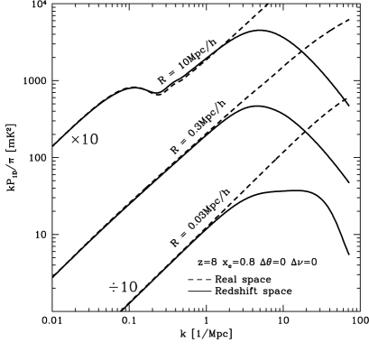
Figure 6.— Real (dashed) and redshift (solid) space 1D power spectra for different fiducial HII patch sizes with perfect angular and frequency resolutions. All parameters are the same except HII patch size $R$. The curves for $R=10h^{-1}{\rm Mpc}$ and $R=0.03h^{-1}{\rm Mpc}$ have been multiplied and divided by 10 respectively for clarity. Note the curves represent the variance of the temperature field in mK² contributed by a logarithmic interval in $k$.

The existence of two scales in the power spectrum means that the detection of a single feature should not automatically be associated with the bubble scale. When $R>\Delta D_{\sigma}$, HII structures always suppress the power spectrum at lower $k$ than the nonlinear redshift space distortion does, so that we can distinguish the HII bubble size signature from the power spectrum. With sufficient radial or frequency resolution we will also be able to observe that FoG distortions lead to a reduction in power that continues to increases with $k$.

The observation of a feature followed by a cutoff in the 1D power spectrum will ensure that the feature is from HII patches. By measuring its evolution in redshift we obtain a statistical measure of the evolution of the typical size of the ionized region. However in the fiducial atomic cooling model with $R=0.3$ $h^{-1}{\rm Mpc}$ only the FoG feature is prominent. In scenarios where $x_{e}$ is also adjusted, the prominence of the bubble feature can be adjusted but a confusion between the two scales can still occur.

If only a single feature is measured and barely resolved then the ambiguity between FoG distortions and bubble size must be broken by measuring the transverse power spectrum. Fortunately, the cosmological redshift space distortion or Alcock-Pacynski effect can be considered known and does not introduce an ambiguity (c.f. Nusser, 2005). Foreground contamination in the transverse dimensions however will have to be controlled.

4. Observed power spectrum

4.1. Modeling experimental resolutions

The observed 21cm power spectrum will also be distorted by instrumental effects from finite angular resolution $\Delta\theta$ and frequency resolution $\Delta\nu$. These modify the 3D power spectrum as

$$P_{\delta T}^{\rm obs}(\vec{k},\Delta\theta,\Delta\nu)=P_{{\delta T}}^{s}(\vec{k})W^{2}_{\Delta\theta}(k_{\perp})W^{2}_{\Delta\nu}(k_{\parallel})\,,$$ (54)

and consequently the projected 1D power spectrum through equation (12). We will take the smoothing due to frequency resolution to be a Gaussian of FWHM $\Delta\nu$ so that

$$W^{2}_{\Delta\nu}(k_{\parallel})=e^{-k_{\parallel}^{2}\delta D^{2}}\,,$$ (55)

where $\delta D$ is given by equation (4) with $\delta\nu=\Delta\nu/\sqrt{8\ln 2}$ to convert the FWHM to a Gaussian width.

For the angular resolution, a single dish experiment with a Gaussian beam of FWHM resolution $\Delta\theta$ would produce a window function

$$W^{2}_{\Delta\theta}(k_{\perp})=e^{-k_{\perp}^{2}D_{\perp}^{2}(\Delta\theta/\sqrt{8\ln 2})^{2}}\,,$$ (56)

where the angular diameter distance is given by equation (5). In our fiducial cosmology, this factor is approximately

$${D_{\perp}\Delta\theta\over\sqrt{8\ln 2}}\approx 1.65{\rm Mpc}\left[1-0.33\left({10\over 1+z}\right)^{1/2}\right]\left({\Delta\theta\over 1^{\prime}}\right)\,,$$ (57)

where we have also converted the angular units from radians to arcminutes on the rhs for convenience.

All planned 21cm experiments are however interferometers. In this case the window function is given by a sharp cutoff in $k_{\perp}$ space defined by the longest baseline. An interferometer array with a maximum baseline of $L$ measures the transverse power spectrum out to

$$k_{\rm cut}={{2\pi L}\over{\lambda D_{\bot}}}\,,$$ (58)

where $\lambda$ is the observation wavelength. With uniform coverage of the baselines, the window function can be approximated as

$$W^{2}_{\Delta\theta}(k_{\perp})=\Big{\{}\begin{array}[]{ll}1&k_{\perp}\leq k_{\rm cut}\,,\\ 0&k_{\perp}>k_{\rm cut}\,.\end{array}$$ (59)

Since the net effect of this sharp cut on the 1D power spectrum is similar to a Gaussian beam of FWHM

$$\Delta\theta = \sqrt{8\ln 2}{\lambda\over 2\pi L}\,,$$ (60)

$$= \sqrt{8\ln 2}{1\over k_{\rm cut}D_{\perp}}\,.$$

we will use the Gaussian window for illustrative purposes in the following sections.

4.2. Observed 1D power spectra

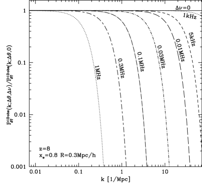
Figure 7.— Ratio of redshift space power spectra with finite frequency resolutions $P^{\rm 1Dobs}_{\delta T}(k;\Delta\theta,\Delta\nu)$ to the one with perfect frequency resolution $P^{\rm 1Dobs}_{\delta T}(k;\Delta\theta,0)$, for a model with parameters $z=8$, $x_{e}=0.8$ and $R=0.3h^{-1}{\rm Mpc}$.

The impact of frequency resolution on the 1D power spectrum is simple in that equations (12) and (54) imply

$$P^{{\rm 1Dobs}}_{\delta T}(k;\Delta\theta,\Delta\nu) = W^{2}_{\Delta\nu}(k)\int{d^{2}k_{\perp}\over(2\pi)^{2}}W^{2}_{\Delta\theta}(k_{\perp})$$ (61)

$$\times P_{{\delta T}}^{s}(\sqrt{k^{2}+k_{\perp}^{2}})\,,$$

so that the relative effect of frequency resolution is independent of the neutral hydrogen model. In 7, we plot $W^{2}_{\Delta\nu}$ or the ratio of 21cm redshift space 1D power spectra for different channel widths $\Delta\nu$ relative to $\Delta\nu=0$. Comparing this figure to the features from the ionization bubbles and the FoG distortions one might naively suppose that the criteria for resolving these depend on $\Delta\nu$ alone.

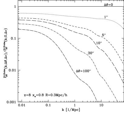
Figure 8.— Ratio of redshift space power spectra with finite angular resolutions $P^{{\rm 1Dobs}}_{\delta T}(k;\Delta\theta,\Delta\nu)$ to the one with perfect angular resolution $P^{\rm 1Dobs}_{\delta T}(k;0,\Delta\nu)$, for a model with parameters $z=8$, $x_{e}=0.8$ and $R=0.3h^{-1}{\rm Mpc}$.

However for projected 1D power spectra, the angular resolution plays an important role. Only modes whose three dimensional wavevector $\vec{k}$ have transverse components that can be resolved contribute to the radial fluctuations in equation (61). Thus a finite angular resolution degrades the 1D signal on all scales and additionally can lead to a new feature in the 1D power spectrum. Figure 8 plots the ratio of redshift space power spectra with different finite effective beam sizes $\Delta\theta$ to the one with $\Delta\theta=0$. Note that the suppression effect is independent of $\Delta\nu$ but does depend on the model 3D power spectrum. Here we have assumed the fiducial $R=0.3$ $h^{-1}$Mpc, $x_{e}=0.8$ model at $z=8$. The feature in Figure 8 near 1 Mpc^-1 is due to the assumed bubble scale. Even with perfect frequency resolution, the angular resolution can mask features from the bubble scale and FoG effects. In the context of foreground removal, 8 implies that for $\Delta\theta\mathrel{\hbox to0.0pt{\lower 3.0pt\hbox{$\mathchar 536\relax$}\hss}\raise 2.0pt\hbox{$\mathchar 318\relax$}}30\arcsec$ the experimental angular resolution will place a more important limitation on cleaning than FoG redshift space distortions.

Note that the total suppression is simply the product of the two curves in Figure 7 and 8. The optimal frequency resolution to extract most of the power in the radial fluctuations is then dependent on angular resolution. Furthermore, we can develop rules of thumb for the instrumental specifications required to unambiguously resolve features such as the FoG effect and the bubble scale as we shall now see.

4.3. Resolving redshift space distortions

For FoG redshift space distortions, the critical scale where all fluctuations will be suppressed is associated with the pairwise velocity dispersion $\sigma_{p}$ since that affects the small scale density contributions. For the ionization fluctuations, $\sigma_{b}$ typically places the suppression scale below that of the bubble scale and hence is less relevant. The pairwise velocity dispersion scale is independent of the bubble model and so leads to robust criteria for its resolution.

Combining 7 with 8, if we have both high frequency resolution $\Delta\nu<0.03{\rm MHz}$ and high angular resolution $\Delta\theta<30\arcsec$, which means both suppress the power at smaller scales than the FoG effect does, we would be able to unambiguously detect the FoG effect in the fiducial model with instrumental sensitivity that can extract mK level signals. More generally, we require that $\delta D\ll\Delta D_{\sigma_{p}}$ and $D_{\perp}\Delta\theta/\sqrt{8\ln 2}\ll\Delta D_{\sigma_{p}}$ to observe nonlinear redshift space distortions at small scales.

Combining equation (4), equation (40), and equation (57), we obtain the rule of thumb on resolution requirements for observing FoG effect in 21cm experiments

$$\Delta\nu\ll\Delta\nu_{\sigma_{p}}=0.034{\rm MHz}\left({{1+z}\over{10}}\right)^{-1}\left({{\sigma_{p}}\over{30\rm{km/s}}}\right)$$ (62)

$$\Delta\theta\ll\Delta\theta_{\sigma_{p}}=8.9\arcsec\left[\left({{1+z}\over{10}}\right)^{1/2}-0.33\right]^{-1}\left({{\sigma_{p}}\over{30\rm{km/s}}}\right)$$ (63)

neglecting the small cosmological dependence and assuming $z\gg 1$. Note that redshift space distortions can only be resolved when both these criteria are satisfied. Likewise for foreground removal, the FoG suppression becomes the limiting factor only if both exceed this criteria.

The characteristic scales defined above decrease with redshift. At $z=8$ where we do all our calculations, assuming $\sigma_{p}=30\rm{km}/s$, equation (62) and equation (63) suggest the characteristic resolutions are $\Delta\nu_{\sigma_{p}}=0.04{\rm MHz}$ and $\Delta\theta_{\sigma_{p}}=14\arcsec$. These results are consistent with 7 and 8.

4.4. Resolving HII regions

We can also establish rules-of-thumb for the resolution of the HII regions or in our model the bubble size $R$. These supplement the considerations in Subsection 3.2 for separability from the FoG scale. We will consequently consider the $R=10h^{-1}{\rm Mpc}$ case where the two scales are themselves well separated.

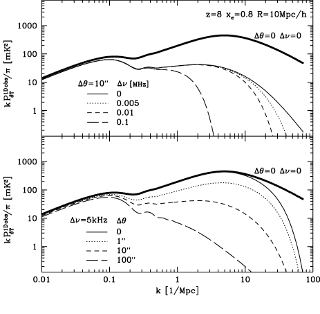
Figure 9.— Redshift space 21cm 1D power spectra for different beam sizes and channel widths, assuming fiducial HII region size $R=10h^{-1}{\rm Mpc}$. For comparison, we also plot power spectra with perfect angular and frequency resolution (thick solid lines).

Figure 9 shows how the redshift space power spectrum changes with different experimental resolutions. With a perfect instrument ($\Delta\theta=0$ and $\Delta\nu=0$) both the larger $R$ scale and the FoG scale are resolved. However, as either increases, the small scale feature is replaced by the instrumental resolution. We can tell from 9 that for $\Delta\nu\lesssim 0.1{\rm MHz}$ and $\Delta\theta\lesssim 100\arcsec$, such large HII structures can be distinguished. It is also interesting to see that when fixing $\Delta\theta=10\arcsec$, it does not help much to improve the frequency resolution beyond $0.01{\rm MHz}$, which implies the requirements for beam size and channel width are correlated in resolving structures, as we pointed out earlier in Subsection 4.2.

More generally, we need both $\delta D\ll R$ and $D_{\perp}\Delta\theta/\sqrt{8\ln 2}\ll R$ to resolve HII structures,

$$\Delta\nu\ll\Delta\nu_{R}=0.14{\rm MHz}\left({{1+z}\over{10}}\right)^{-1/2}\left({{R}\over{{\rm Mpc}}}\right)$$ (64)

$$\Delta\theta\ll\Delta\theta_{R}=36.4\arcsec\left[1-0.33\left({{10}\over{1+z}}\right)^{1/2}\right]^{-1}\left({{R}\over{{\rm Mpc}}}\right)$$ (65)

Either resolution not satisfying the above conditions will result in a smearing scale larger than HII scale so that the feature will be obscured.

Furthermore, because of the existence of redshift space distortions, $R$ and $D_{\sigma}$ can lead to degenerate effects as we have already discussed in Subsection 3.2. Thus the required resolutions for observing any structures, either HII patches, or finger-of-God features, are the results of minimizing equation (62) and equation (64), plus equation (63) and equation (65), respectively.

5. Considerations for experiments

5.1. An ultimate experiment

In order to fully take advantage of all data, and go beyond the foreground dominated region to remove foreground efficiently (Wang et al., 2005), we would of course like to get as good angular and frequency resolution as possible. On the other hand, with a reasonable ionization model like that established here there are guides to when an instrument will recover essentially all of the useful cosmological signal.

In the absence of redshift space distortions, we have seen that the predicted temperature fluctuations continue to rise in rms as the frequency resolution increases due to density fluctuations outside of the ionization bubbles. This would imply that to be most immune to smooth foregrounds in frequency space, one should concentrate the instrumental sensitivity in as small a frequency band and field as possible. However, we have seen that FoG smoothing in the radial direction will generically introduce a cutoff in the observed power and set a lower limit of $\Delta\nu\sim 10$kHz on the required frequency resolution. To match this frequency resolution one would desire an angular resolution of $\Delta\theta=10^{\prime\prime}$ although there are gains all the way out to $\Delta\theta=1^{\prime\prime}$.

Table 1 Resolution requirements for future “ideal” experiments

Resolve	$R>\Delta D_{\sigma_{p}}$	$R<\Delta D_{\sigma_{p}}$
$R$	$\Delta\theta_{\sigma_{p}}<\Delta\theta<\Delta\theta_{R}$	Not applicable
	$\Delta\nu_{\sigma_{p}}<\Delta\nu<\Delta\nu_{R}$
FoG	$\Delta\theta<\Delta\theta_{\sigma_{p}}(<\Delta\theta_{R})$	$\Delta\theta<\Delta\theta_{\sigma_{p}}$
	$\Delta\nu<\Delta\nu_{\sigma_{p}}(<\Delta\nu_{R})$	$\Delta\nu<\Delta\nu_{\sigma_{p}}$
Both	$\Delta\theta<\Delta\theta_{\sigma_{p}}(<\Delta\theta_{R})$	Not applicable
	$\Delta\nu<\Delta\nu_{\sigma_{p}}(<\Delta\nu_{R})$

The requirements on resolving ionization bubbles are more model dependent. The best case scenario is that the HII patches are larger than the characteristic scale introduced by the velocity dispersion as one would expect near the end of reionization. Under this scenario, HII patches can be resolved without ambiguities from redshift space distortions and the experimental requirements can be relaxed to satisfy $\Delta\theta<\Delta\theta_{R}$ and $\Delta\nu<\Delta\nu_{R}$. In the unfortunate scenario when $R<\Delta D_{\sigma_{p}}$, e.g., if reionization ends with the creation of many small ionization regions or the observation redshift is too high, radial resolution of HII structures will be difficult even with perfect experimental resolutions.

Table 1 summarizes our angular and frequency resolutions considerations. Note that the signal to noise will also have to be high enough to detect the $\sim 10$ mK signals in question.

5.2. First generation experiments

The first generation 21 cm experiments will be far from the ultimate angular resolution at the required signal to noise levels considered in the previous section. We discuss here what the impact of redshift space modeling will be for these experiments.

The upcoming MWA (Mileura Widefield Array) experiment has $8{\rm kHz}$ frequency resolution which is in fact sufficient for even our ultimate experiment. At $200{\rm MHz}$ ($z=6.1$), its beam size is $3.4\arcmin$. The characteristic resolutions at this redshift for resolving HII structures and observing FoG effects are given by equations (62)-(65) as $\Delta\nu_{R}=0.17{\rm MHz}(R/{\rm Mpc})$, $\Delta\theta_{R}=60\arcsec(R/{\rm Mpc})$, $\Delta\nu_{\sigma_{p}}=0.05{\rm MHz}(\sigma_{p}/30\rm{{\rm km}s^{-1}})$, and $\Delta\theta_{\sigma_{p}}=17\arcsec(\sigma_{p}/30\rm{{\rm km}s^{-1}})$. These results suggest that MWA will be able to observe HII patches larger than $\sim 3{\rm Mpc}$. It also implies that the FoG redshift space distortions will not be the limiting factor in foreground removal as long as the average velocity dispersion at that time is less than $\sim 350\rm{km/s}$, as expected in any reasonable model.

At $100{\rm MHz}$ ($z=13.2$), MWA can achieve an angular resolution $\sim 6.8\arcmin$. The characteristic resolutions at this redshift are $\Delta\nu_{R}=0.12{\rm MHz}(R/{\rm Mpc})$, $\Delta\theta_{R}=50\arcsec(R/{\rm Mpc})$, $\Delta\nu_{\sigma_{p}}=0.02{\rm MHz}(\sigma_{p}/30\rm{{\rm km}s^{-1}})$, and $\Delta\theta_{\sigma_{p}}=10\arcsec(\sigma_{p}/30\rm{{\rm km}s^{-1}})$. Similarly, it will not be able to resolve HII regions if they are smaller than $\sim 8{\rm Mpc}$ and FoG distortions are even less of a limiting factor for foreground removal.

Another upcoming experiment LOFAR, has frequency resolution $4{\rm kHz}$, angular resolution $3.1\arcmin$ for virtual core setup at $200{\rm MHz}$, and $5.2\arcmin$ at $120{\rm MHz}$. At 200 MHz ($z=6.1$), it will be able to observe HII regions larger than $\sim 3{\rm Mpc}$, yet will not be affected by FoG distortions as long as $\sigma_{p}<300{\rm km}/s$. Similarly, at 120MHz ($z=10.8$), it will resolve HII regions which are larger than $\sim 6{\rm Mpc}$.

Improving the angular resolution with longer baselines can only improve these numbers before the characteristic scale for FoG distortions is reached $\Delta D_{\sigma}=0.3{\rm Mpc}(\sigma/30\rm{kms^{-1}})$. If HII bubbles are smaller than this scale at the corresponding redshift, we are unable to unambiguously resolve them from their radial structure no matter how good the resolutions are. This complication may impact the next generation experiment beyond MWA and LOFAR.

In conclusion, for both LOFAR and MWA, the complication arising from nonlinear redshift space distortions in foreground cleaning should be minimal. Both experiments can detect large HII structures and their correlations at the end of reionization epoch. Yet it could be difficult for them to distinguish smaller patches expected at earlier times.

One should also bear in mind that the actual ability of individual experiments to distinguish HII regions also depends on many other factors such as quality of foreground cleaning, treatment of systematics, signal-to-noise ratio, etc. Experimental resolution is only one of many factors that determine how much information from the reionization epoch can be extracted from the observational data.

6. Summary

In this paper, we construct a self-consistent analytic model for 21cm brightness temperature power spectrum in the observed redshift space domain. In its simplest form, our model has two input parameters at each redshift, the average ionization fraction and HII bubble size. It can be readily generalized to consider a distribution of bubble sizes with various profiles while maintaining the proper scalings with ionization fraction. Though still a toy model of reionization, it is easy to apply to rapidly explore alternatives and has the flexibility to accommodate various physical reionization mechanisms, including those based on atomic line cooling.

Utilizing this model, we study the 1D power spectrum along the line of sight. Given that foreground contamination is expected to be smooth in frequency space, the 1D structure of the brightness temperature is the most robust observable and a likely stepping stone for constructing the foreground cleaned 3D maps.

We show the existence of redshift space distortions will eventually limit our ability to observe epoch of reionization. When the average size of HII regions is smaller than the characteristic scale of the average velocity dispersion, as is likely toward the beginning of reionization, they can not be radially resolved. Furthermore at the low ionization levels typical of the beginning of reionization, the brightness fluctuations will be dominated by density fluctuations. Features due to the presence of HII regions may be masked by even relatively small uncertainties in the redshift space distortions.

Combining the radial structure induced by the HII bubbles and nonlinear redshift space distortions, we outline criteria for planning the angular and frequency resolution of experiments. Even in the 1D spectra, angular resolution enters by eliminating contributions from modes that are not purely radial thus degrading the signal. It is a serious limiting factor for the first generation experiments such as MWA and LOFAR. For such experiments, only HII bubbles that are larger than a few Mpc can be radially resolved even with ideal frequency resolution. On the other hand, nonlinear redshift distortions will not seriously affect such experiments. They do however suggest that for future experiments a frequency resolution of $\sim 10$kHz and an angular resolution of 10″ will be sufficient to extract most of the information from the radial power spectrum near the end of reionization.

Appendix A Distribution of Bubble Sizes

A distribution of bubble sizes can be straightforwardly accommodated in the framework of our model following Mortonson & Hu (2006). Let us denote the probability of obtaining a bubble of radius within $dR$ of $R$ as $P(R)dR$. The ionization fraction associated with this bubble distribution is given by

$$x_{e} = 1-e^{-\bar{n}_{b}\langle V_{b}\rangle}\,,$$ (A1)

where the average bubble volume is

$$\langle V_{b}\rangle = \int dRP(R)V_{b}(R)\,.$$ (A2)

The window functions in one and two bubble term power spectra calculations are also replaced by average values. For two bubble terms, $W_{R}$ in equation (24) becomes

$$\langle W_{R}\rangle={1\over{\langle V_{b}\rangle}}\int dRP(R)V_{b}(R)W_{R}\ .$$ (A3)

For one bubble terms, $W_{R}^{2}$ in equation (29) is replaced by

$$\langle W_{R}^{2}\rangle={1\over{\langle V_{b}\rangle^{2}}}\int dRP(R)V^{2}_{b}(R)W^{2}_{R}\ .$$ (A4)

Note that the approximation to the convolution term in equation (33) still holds with $\sigma_{R}^{2}$ becoming

$$\langle\sigma_{R}^{2}\rangle={1\over{\langle V_{b}\rangle^{2}}}\int dRP(R)V^{2}_{b}(R)\sigma_{R}^{2}\,.$$ (A5)

There are two qualitative effects of including a distribution. The averaging process removes the ringing of the 3D power spectra and broadens the feature associated with the bubble size. It also can change the relative strengths of the one and two bubble contributions. For example, since

$$\lim_{k\rightarrow 0}{\langle W_{R}^{2}\rangle\over\langle W_{R}\rangle^{2}}\rightarrow{\langle V_{b}^{2}\rangle\over\langle V_{b}\rangle^{2}}\,,$$ (A6)

the larger bubbles in the distribution enhance the power in the one bubble term at low $k$.

To make these considerations concrete, let us consider a lognormal distribution

$$P(R)={1\over R}{1\over{\sqrt{2\pi}\sigma_{\ln R}}}\exp{\left[{{(\ln R-\ln R_{0}+3\sigma^{2}_{\ln R}/2)^{2}}\over{2\sigma^{2}_{\ln R}}}\right]}\,,$$ (A7)

where the offset is defined so that $\langle V_{b}\rangle=V_{0}=4\pi R_{0}^{3}/3$ and similarly, $\langle V_{b}^{2}\rangle=V_{0}^{2}\exp{(9\sigma^{2}_{\ln R})}$. Numerical simulations suggest that a reasonable range for $\sigma_{\ln R}$ is $[0.5,1]$ (Furlanetto, McQuinn, & Hernquist, 2005).

In 10, we show the 1D and 3D real space power spectra for several values of $\sigma_{\ln R}$ and two choices of $R_{0}$. In the 3D case, all oscillations are averaged away and also the bubble transition takes place over a wide range of scales extending out to $\ln R\approx\ln R_{0}+3\sigma_{\ln R}^{2}/2$ due to the scaling of $\langle V_{b}^{2}\rangle$. Analogous effects occur for the 1D power spectra and the shift in the transition scale toward larger scales can make the bubble transition slightly more prominent. Nevertheless the qualitative conclusions of the main paper remain unchanged once an allowance has been made for the effective characteristic bubble scale.

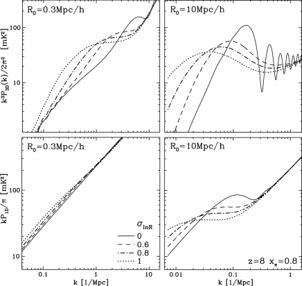
Figure 10.— Dependence of 3D (top) and 1D (bottom) real space power spectra on the width of the bubble radii distribution $\sigma_{\ln R}$ for two choices of $R_{0}=0.3$Mpc$/h$ (left) and $10$Mpc$/h$ (right). Note that oscillations in the 3D spectra are averaged out and the feature due to the bubbles is drawn out and extends to larger scales. Models are evaluated at $z=8$ with $x_{e}=0.8$.

References

- (1)
- Barkana (2005) Barkana, R. 2005, astro-ph/0508341
- Barkana & Loeb (2005a) Barkana, R. and Loeb, A. 2005, ApJ, 624, L65
- Barkana & Loeb (2005b) Barkana, R. and Loeb, A. 2005, ApJ, 626, 1
- Barkana & Loeb (2004) Barkana, R. and Loeb, A. 2004, ApJ, 609, 474
- Barkana, Haiman, & Ostriker (2001) Barkana, R., Haiman, Z., and Ostriker, J. P. 2001, ApJ, 558, 482
- Becker et al. (2001) Becker, R. H. et al. 2001, AJ, 122, 2850
- Bharadwaj & Ali (2005) Bharadwaj, S. and Ali, S. 2005, MNRAS, 356, 1519
- Bullock et al. (2001) Bullock, J. S. et al. 2001, MNRAS, 321, 559
- Carilli (2005) Carilli, C. L. 2005, astro-ph/0509055
- Chen & Miralda-Escude (2004) Chen, X. and Miralda-Escude, J. 2004, ApJ, 602, 1
- Ciardi & Madau (2003) Ciardi, B. and Madau, P. 2003, ApJ, 596, 1
- Cooray (2004) Cooray, A. 2004, astro-ph/0411430
- Cooray & Sheth (2001) Cooray, A. and Sheth, R. 2001, Phys. Rep., 372, 1
- Desjacques & Nusser (2004) Desjacques, V. and Nusser, A. 2004, MNRAS, 351, 1395
- Fan et al. (2002) Fan, X. et al. 2002, AJ, 123, 1247
- Furlanetto, McQuinn, & Hernquist (2005) Furlanetto, S. R., McQuinn, M., and Hernquist, L. 2005, astro-ph/0507524
- Furlanetto, Sokasian, & Hernquist (2004) Furlanetto, S. R., Sokasian, A., and Hernquist, L. 2004, MNRAS, 347, 187
- Furlanetto, Zaldarriaga, & Hernquist (2004a) Furlanetto, S., Zaldarriaga, M., and Hernquist, L. 2004, ApJ, 613, 1
- Furlanetto, Zaldarriaga, & Hernquist (2004) Furlanetto, S., Zaldarriaga, M., and Hernquist, L. 2004, ApJ, 613, 16
- Gnedin & Shaver (2004) Gnedin, N. Y. and Shaver, P. A. 2004, ApJ, 608, 611
- Gruzinov & Hu (1998) Gruzinov, A. and Hu, W. 1.998, ApJ, 508, 435;astro-ph/9803188
- Gunn & Peterson (1965) Gunn, J. E. and Peterson, B. A. 1965, ApJ, 142, 1633
- Haiman & Holder (2003) Haiman, Z. and Holder, G. P. 2003, ApJ, 595, 1
- Haiman (2003) Haiman, Z. 2003, astro-ph/0304131
- Hamilton (1997) Hamilton, A. J. S. 1997, astro-ph/9708102
- Hamilton (2001) Hamilton, A. J. S. 2001, MNRAS, 322, 419
- Hogan & Rees (1979) Hogan, C. J. and Rees, M. J. 1979, MNRAS, 188, 791
- Kaiser (1987) Kaiser, N. 1987, MNRAS, 227, 1
- Kogut et al. (2003) Kogut, A. et al. 2003, ApJS, 148, 161
- Lahav et al. (1991) Lahav, O., Lilje, P. B., Primack, J. R., and Rees, M. J. 1991, MNRAS, 251, 128
- Loeb & Barkana (2000) Loeb, A. and Barkana, R. 2000, astro-ph/0010467
- Madau, Meiksen &Rees (1997) Madau, P., Meiksin, A., and Rees, M. J. 1997, ApJ, 475, 429
- Miralda-Escude, Haehnelt, & Rees (2000) Miralda-Escude, J., Haehnelt, M., and Rees, M. J. 2000, ApJ, 530, 1
- Morales (2005) Morales, M. F. 2005, ApJ, 619, 678
- Morales, Bowman, & Hewitt (2005) Morales, M. F., Bowman, J. D., and Hewitt, J. N. 2005, astro-ph/0510027
- Morales & Hewitt (2003) Morales, M. F. and Hewitt, J. 2004, ApJ, 615, 7
- Mortonson & Hu (2006) Mortonson, M. & Hu W, in preparation.
- Navarro, Frenk, & White (2004) Navarro, J. F., Frenk, C. S. , and White, S. D. M. 1997, ApJ, 490, 493
- Nusser (2005) Nusser, A. 2005, MNRAS, 364, 743
- Oh & Mack (2003) Oh, S. P. and Mack, K. J. 2003, MNRAS, 346, 871
- Pen, Wu, & Peterson (2004) Pen, U-L., Wu, X-P., and Peterson, J. 2004, astro-ph/0404083
- Santos et al. (2003) Santos, M. G., Cooray, A., Haiman, Z., Knox, L. , and Ma, C-P. 2003, ApJ, 598, 756
- Santos, Cooray, & Knox (2005) Santos, M. G., Cooray, A., and Knox, L. 2005, ApJ, 625, 575
- Scoccimarro (2004) Scoccimarro, R. 2004, Phys. Rev. D, 70, 083007
- Scott & Rees (1990) Scott, D. and Rees, M. J. 1990, MNRAS, 247, 510
- Seljak et al. (2005) Seljak, et al.. 2005, Phys. Rev. D, 71, 103515
- Sheth (1996) Sheth, R. 1996, MNRAS, 279, 1310
- Sheth & Tormen (1999) Sheth, R. K. and Tormen, G. 1999, MNRAS, 308, 119
- Somerville, Bullock & Livio (2003) Somerville, R. S., Bullock, J. S., and Livio, M. 2003, ApJ, 593, 616
- Spergel et al. (2003) Spergel, D. N. et al. 2003, ApJS, 148, 175
- Tegmark et al. (2004) Tegmark, M. et al. 2004, Phys. Rev. D, 69, 103501
- Tinker, Weinberg & Zheng (2005) Tinker, J. L., Weinberg, D. H., and Zheng, Z. 2005, astro-ph/0501029
- Wang et al. (2005) Wang, X., Tegmark, M., Santos, M., and Knox, L. 2005, astro-ph/0501081
- White (2001) White, M. 2001, MNRAS, 321, 1
- Wyithe & Loeb (2004b) Wyithe, S. and Loeb, A. 2004, Nature, 432, 194
- Yoshida et al. (2003) Yoshida, N., Abel, T., Hernquist, L. , and Sugiyama, N. 2003, ApJ, 592, 642
- Zaldarriaga, Furlanetto, & Hernquist (2004) Zaldarriaga, M., Furlanetto, S. R., and Hernquist, L. 2004, ApJ, 608, 622