On the nitrogen abundance of FLIERs: the outer knots of the planetary nebula NGC 7009

Abstract

We have constructed a 3D photoionisation model of a planetary nebula (PN) similar in structure to NGC 7009 with its outer pair of knots (also known as FLIERs –fast, low-ionization emission regions). The work is motivated by the fact that the strong [N ii]$\lambda$6583 line emission from FLIERs in many planetary nebulae has been attributed to a significant local overabundance of nitrogen. We explore the possibility that the apparent enhanced nitrogen abundance previously reported in the FLIERs may be due to ionization effects. The model is constrained by the results obtained by Gonçalves, Corradi, Mampaso & Perinotto (2003) from the analysis of both HST [O iii] and [N ii] images, and long-slit spectra of NGC 7009. Our model is indeed able to reproduce the main spectroscopic and imaging characteristics of NGC 7009’s bright inner rim and its outer pairs of knots, assuming homogeneous elemental abundances throughout the nebula, for nitrogen as well as all the other elements included in the model.

We also study the effects of a narrow slit on our non-spherically symmetric density distribution, via the convolution of the model results with the profile of the long-slit used to obtain the spectroscopic observations that constrained our model. This effect significantly enhances the [N ii]/H$\beta$ emission, more in the FLIERs than in the inner rim.

Because of the fact that the (N⁺/N)/(O⁺/O) ratio predicted by our models are 0.60 for the rim and 0.72 for the knots, so clearly in disagreement with the N⁺/N=O⁺/O assumption of the ionization correction factors method (icf), the icfs will be underestimated by the empirical scheme, in both components, rim and knots, but more so in the knots. This effect is partly responsible for the apparent inhomogeneous N abundance empirically derived. The differences in the above ratio in these two components of the nebula may be due to a number of effects including charge exchange –as pointed out previously by other authors– and the difference in the ionization potentials of the relevant species –which makes this ratio extremely sensitive to the shape of the local radiation field. Because of the latter, a realistic density distribution is essential to the modelling of a non-spherical object, if useful information is to be extracted from spatially resolved observations, as in the case of NGC 7009.

1 Introduction

Table 1: Main physical/chemical parameters from Paper i.

Parameter	R		K		NEB
	Eastern	Western	Eastern	Western	Whole Nebula
Ne[S ii](cm-3)	5,500	5,900	2,000	1,300	4,000
Ne[Cl iii](cm-3)	5,200	5,900	-	1,900	1,300
Te[O iii](K)	10,000	10,200	9,600	10,400	10,100
Te[N ii](K)	10,400	12,800	11,000	11,700	10,300
Te[S ii](K)	-	-	7,100	9,400	-
He/H	1.08(-1)	1.16(-1)	1.02(-1)	9.55(-2)	1.11(-1)
O/H	4.5(-4)	4.82(-4)	5.8(-4)	4.5(-4)	4.71(-4)
N/H	7.0(-5)	1.8(-4)	3.8(-4)	2.5(-4)	1.7(-4)
Ne/H	1.1(-4)	1.1(-4)	1.1(-4)	1.3(-4)	1.1(-4)
S/H	6.1(-6)	4.9(-6)	1.39(-5)	9.3(-6)	8.3(-6)

Empirically derived parameters, for the different structures of the NGC 7009, for both, the Eastern and Western sides of the nebula, with “R”, “K” and “NEB” standing for rim, outer knots and the whole nebula (see Tables 1 and 3 of Paper i).                                                                   

It is well known that planetary nebulae (PNe) possess a number of small-scale structures that, at variance with their large-scale structures, are prominent in low-ionization emission lines, such as [N ii] and [O ii]. In terms of morphology and kinematics, the low-ionization structures (LISs, for a review see Gonçalves, 2004) may appear as knots, filaments, jets, and isolated features that, in some cases, move with the same velocity of the ambient nebula, or supersonically through the environment, like FLIERs (fast, low-ionization emission regions, Balick et al., 1993) or BRETs (bipolar, rotating, episodic jets; López et al., 1995).

For over ten years, the strong [N ii] line emission from LISs has been attributed to a significant local overabundance of nitrogen (Balick et al. 1993, 1994, 1998; and references therein). Balick et al. (1993) interpreted the N-enrichment in FLIERs as evidence of their origins in recent high-velocity ejections of the PN central star. The above work and successively Balick et al. (1994), which included the derivation of the ionic and elemental abundances of LISs, pointed out “an apparent enhancement of nitrogen relative to hydrogen by factors of 2-5” in FLIERs. However, since then, further work casted doubts over the latter statement (Hajian et al., 1997; Alexander & Balick, 1997; Gonçalves et al., 2003; Perinotto et al., 2004a).

Abundances in PNe can be derived from the analysis of collisionally excited line (CEL) or optical recombination line (ORL) spectra using empirical methods or tailored photoionisation models (e.g. Stasińska, 2004) or a combination of the two. For some elements (e.g. He) and ions (e.g. N⁺⁺ if only the optical spectrum is available) the use of ORL is mandatory, whilst for others the use of CELs may be unavoidable. But, when both CEL and ORL determinations are available, the former have been commonly preferred because they are generally stronger and easier to detect than ORLs. Moreover, there is a well known discrepancy between CEL- and ORL-abundances, as well as electron temperature determinations (Liu et al., 1995). Empirical abundance analysis rely on ionization correction factors (icfs) to account for the unseen ions (e.g. Kingsburgh & Barlow, 1994). Results obtained with the icf method can be somewhat uncertain in some cases, particularly when they are applied to spatially resolved long-slit spectra (Alexander & Balick, 1997), as has been the case for the work of Balick et al. (1994); Hajian et al. (1997) and Gonçalves et al. (2003, hereafter Paper i).

In fact, the abundances derived in Paper i and shown here in Table 1, from optical long-slit spectra of NGC 7009, using the icf scheme of Kingsburgh & Barlow (1994), showed only a marginal evidence for overabundance of N/H in the outer knots of the nebula (the ansae), reinforcing the doubts over previous results (Balick et al., 1994) where the N/H enhancement of a factor of 2-5 in the ansae were reported.

One of the major shortcomings of empirically-determined chemical abundances lies in the fact that a number of assumptions on the ionization structure of the gas need to be made in order to obtain the icfs. A preferred alternative would be the construction of a tailored photoinisation model for a given object, aiming to fit the emission line spectrum and, in the case of spatially resolved objects, projected maps in a number of emission lines.

NGC 7009, the “Saturn Nebula”, is a PN comprising a bright elliptical rim. Its small-scale structures include a pair of jets and two pairs of low-ionization knots. On a larger scale, it is known that NGC 7009 possess a tenuous halo with a diameter of more than 4 arcmin (Moreno et al., 1998), whose inner regions display a system of concentric rings (Corradi et al., 2004) like those observed in NGC 6543 and other few PNe (Balick et al, 2001). High-excitation lines dominate the inner regions along the minor axis, while emission from low-ionization species is enhanced at the extremities of the major axis. The ionization structure is further enriched by the fact that the low-excitation regions present strong variations in excitation level and clumpiness. NGC 7009 was classified as an oxygen-rich PN (Hyung & Aller, 1995a), with an O/C ratio exceeding 1, and anomalous N, O, and C abundances (Baker, 1983; Balick et al., 1994; Hyung & Aller, 1995a). Its central star is an H-rich O-type star, with effective temperature of 82 000 K (Méndez et al., 1992; Kingsburgh & Barlow, 1992). The kinematics of NGC 7009 was studied first by Reay & Atherton (1985) and Balick et al. (1987), who showed that the ansae are expanding near the plane of the sky at highly supersonic velocities. The derived inclination of the inner (caps) and outer (ansae) knots, with respect to the line of sight, are $i\cong 51^{\circ}$ and $i\cong 84^{\circ}$, respectively (Reay & Atherton, 1985). More recently, Fernández et al. (2004) have measured the proper motion and kinematics of the ansae in NGC 7009, assuming that they are equal and opposite from the central star, obtaining V_exp = 114 $\pm$ 32  km s^-1, for the distance of $\sim$ 0.86 $\pm$ 0.34 kpc.

In this paper we will present a simple 3D photoionisation model, aiming at reproducing the observed geometry and spectroscopic “peculiarities” of a PN like NGC 7009, exploring the possibility that the enhanced [N ii] emission observed in the outer knots may be due to ionization effects. We will use the 3D photoinisation code mocassin (Ercolano et al., 2003a) together with the long-slit data presented in Paper i and the HST images available for this nebula. Our model and the observational data are described in Section 2. The results for our main model are presented and discussed in Section 3, while in Section 4 we discuss an alternative model, aimed at highlighting the relevance of the geometry and density distribution in such a kind of modelling. The work is briefly summarised in Section 5, where our final conclusions are also stated.

2 Method

2.1 Observational data

The observations used to constrain the photoionisation model were described in detail in Paper i. These included HST [O iii] and [N ii] images as well as Isaac Newton Telescope long-slit, intermediate dispersion spectra, along the PN major axis (P.A. = 79^∘). For further details see Paper i.

We refer to Figure 1 of Paper i, the HST [O iii] and [N ii] images of NGC 7009, in which the nebular features are outlined. Here we will employ the same nomenclature introduced in Paper i. See also the left panel of Figure 2, in Section 3.5.

2.2 The 3D photoionisation code: mocassin

The nebula was modeled using the 3D photoinisation code, mocassin, of Ercolano et al. (2003a). The code employs a Monte Carlo technique to the solution of the radiative transfer of the stellar and diffuse field, allowing a completely geometry-independent treatment of the problem without the need of imposing symmetries or approximations for the transfer of the diffuse component.

The reliability of the code was demonstrated via a set of benchmarks described by Péquignot et al. (2001) and Ercolano et al. (2003a). A number of axy-symmetric planetary nebulae have already been modeled using mocassin, examples include NGC 3918 (Ercolano et al., 2003b), NGC 1501 (Ercolano et al., 2004) and the H-deficient knots of Abell 30 (Ercolano et al., 2003c).

2.3 Input parameters

Table 2: Input parameters for the model.

L∗ ($L_{\odot}$)	3136	N/H	2.0(-4)
Teff (K)	80,000	O/H	4.5(-4)
Rin (cm)	0.0	Ne/H	1.06(-4)
Rout (cm)	3.88(17)	S/H	0.9(-5)
He/H	0.112	Ar/H	1.2(-6)
C/H	3.2(-4)	Fe/H	5.0(-7)

Abundances are given by number, relative to H.

A thorough investigation of the vast parameter space was carried out in this work. This involved experimenting with various gas density distributions, central star parameters and nebular elemental abundances. The model input parameters that best fitted all observational constraints are summarised in Table 2, and discussed in more detail in the following subsections.

A common problem when studying galactic PNe is the large uncertainties associated with the distance estimates, that propagate to the determination of the nebula geometry and central star parameters. We adopted a distance of 0.86 kpc for our models of NGC 7009, as computed by Fernández et al. (2004) from the weighted average of 14 values (Acker et al., 1992) determined with statistical methods; the value was quoted with an error of $\pm$ 0.34 kpc.

2.3.1 Stellar parameters

After having experimented with various stellar atmosphere models to describe the ionising continuum, we reverted to using a blackbody of T_eff = 80,000 K and $\log$ L_∗ = 3.50, as this resulted in the best fit of the nebular emission line spectrum. Méndez et al. (1992) determined the T_eff and $\log$ g for the central star of NGC 7009 using non-LTE model atmosphere analysis of the stellar H and He absorption line profiles, finding T_eff = 82 000 K and $\log$ L_∗ = 3.97, in solar units. Méndez et al. (1992) assumed a distance of 2.1 kpc in their analysis which therefore resulted in their value for the stellar luminosity being higher than that inferred from our modelling.

2.3.2 Elemental Abundances

The nebular elemental abundances used for the photoionisation model are listed in Table 2, where they are given by number with respect to H. Although the mocassin code can handle chemical inhomogeneities, these were not included in our models as they proved to be not necessary to reproduce the CEL spectra of the R and K regions of NGC 7009.

The values shown result from an iterative process, where the initial guesses at the elemental abundances of He, N, O, Ne and S, taken from Paper i (see Table 1), and those of C and Ar, from Pottasch (2000), were successively modified to fit the spectroscopic observations.

2.3.3 Density distribution

The simplest possible density distribution model was constructed in order to demonstrate that the spectroscopic peculiarities often found in LISs can be the product of simple (and well-known) photoionisation effects. The case of NGC 7009 is taken as an example, but the emphasis is not in the construction of a detailed model for this object in particular. With this in mind we described the nebula by an ellipsoidal rim with a H number density, N_H, peaking to 9000 cm^-3 in the short axis direction exponentially decreasing to a minimum value of 4000 cm^-3 in the long axis direction. The short and long axes of the inner and outer ellipsoids measure 3.84$\times$10¹⁶ cm and 9.99$\times$10¹⁶ cm, and 7.06$\times$10¹⁶ cm and 1.84$\times$10¹⁷ cm, respectively, at the distance assumed for NGC 7009. The rim is surrounded by a spherical shell of less opaque, homogeneous density gas, with N_H = 1600 cm^-3. The diameter of the sphere is equal to the long axis of the outer ellipsoid defining the rim. Cylindrical jets, 1.75$\times$10¹⁶ cm in diameter, connect the rim to a pair of disk-shaped knots aligned at a distance of 3.49$\times$10¹⁷ cm from the central star, along the long axis of the ellipsoid. The cylindrical jets widen into cone-shapes at the knot ends in order to simulate the effect of material accumulating at the knots, as suggested by the $HST$ images (particularly for knot K4, as seen in the right panels of Figure 2). The diameter of the base of the cones equals that of the disk-shaped knots. The centres of the 3.49$\times$10¹⁶ cm diameter circular disks representing the knots are aligned with the centres of the cylindrical jets (hence they are seen almost edge on). The width of the disks is assumed to be 3.88$\times$10¹⁶ cm in our model, although only a fraction of these is ionised, as is clear from the right panels of Figure 2. The H number density in the jets and knots is taken to be homogeneous and equal to 1250 cm^-3 and 1500 cm^-3, respectively, consistently with the values derived in Paper i.

Results from the ellipsoidal rim and the spherical outer shell are combined into a single R-component to enable us to carry out a direct comparison with the slit spectra from Paper i, as we show in Table 1.

The jets (J-component) are included in our simulation as the radiation field has to be transferred through them before reaching the outer ansae (K-component). However, given that the emission detected from this region is very faint and that such structures may not be in equilibrium, we take our results for the J-component as very uncertain and omit them from any further discussion.

Finally, neither the inner caps nor the tenuous halo were included in our model. The former because they do not lie on the same axis as the K-component (Reay & Atherton, 1985), and are therefore not expected to have a major influence on the ionization structure of the outer knots. And the latter because it is very faint, and therefore it is not expected to contribute significantly to the integrated emission line spectrum.

Figure 1 shows model profiles along the major axis, in agreement with our assumed density, as N_e/N_H ratio is correlated to the level of ionisation of the gas (see Section 3.4).

Table 3: Model and observed dereddened spectra of R, K and NEB. Line intensities are normalized to H$\beta$=100.

Line Identification (Å)	R			K			NEB
	Model	Model	Obs.	Model	Model	Obs.	Model	Model	Obs.
	no-slit	slit		no-slit	slit		no-slit	slit
H$\beta$(10-13 erg cm-2 s-1)	3119	397.1	-	7.93	2.94	-	3136	405.7	3197*
[Oii] 3726.0 + 3728.8	5.38	5.88	15.5	213.	241.	204.	6.06	8.21	24.2
			7.34			155.
[Neiii] 3868.7	111.	112.	106.	131.	129.	82.3	111.	113.	108.
			105.			141.
**[Neiii] 3967.5	34.5	34.8	51.7	40.5	40.1	35.3	34.6	34.9	48.9
			44.6			59.8
[Sii] 4068.6	0.31	0.35	1.50	4.95	5.46	7.43	0.33	0.40	1.98
			2.36			5.04
[Sii] 4076.4	0.10	0.11	0.87	1.63	1.80	2.36	0.10	0.13	1.11
			1.16			1.83
[Oiii] 4363.2	8.54	8.55	7.76	10.2	9.88	6.94	8.55	8.59	8.15
			8.65			9.64
Heii 4685.7	16.8	22.0	26.0	0.00	0.00	1.00	16.7	21.6	15.8
			23.4			1.23
**[Ariv] 4711	3.92	3.87	5.48	1.50	1.40	2.19	3.91	3.84	4.10
			4.96			2.00
[Ariv] 4740.2	5.19	5.24	5.56	1.27	1.19	1.14	5.17	5.18	3.92
			4.54			1.49
H$\beta$ 4861.3	100.	100.	100.	100.	100.	100.	100.	100.	100.
			100.			100.
[Oiii] 5006.8	1197	1172	1162	1315	1272	1238	1198	1177	1206
			1225			1310
[Cliii] 5517.7	0.35	0.36	0.43	1.09	1.08	0.00	0.35	0.37	0.54
			0.43			0.97
[Cliii] 5537.9	0.57	0.59	0.53	1.04	1.03	0.00	0.57	0.59	0.64
			0.55			0.90
[Nii] 5754.6	0.10	0.11	0.14	3.04	3.48	6.49	0.11	0.15	0.46
			0.18			3.91
Hei 5875.7	14.1	13.4	13.9	15.8	15.9	18.8	14.1	13.5	14.5
			14.1			15.0
[Siii] 6312.1	1.47	1.55	1.27	4.04	3.99	3.89	1.48	1.59	1.68
			1.14			3.25
[Nii] 6583.4	5.87	6.64	7.09	167.	193.	355.	6.39	8.44	27.
			5.60			194.
Hei 6678.1	3.99	3.82	3.87	4.48	4.49	7.49	3.99	3.83	3.97
			3.95			3.18
[Sii] 6716.5	0.46	0.53	0.48	21.9	24.2	36.8	0.53	0.79	2.33
			0.38			23.2
[Sii] 6730.8	0.84	0.99	0.84	29.3	32.4	51.0	0.94	1.32	3.85
			0.69			28.4

The Model spectra are given with and without considering the narrow slit effect. Upper rows give the observed intensities of the North-East (R1 and K1) part of the nebula, while those for the South-West (R2 and K4) zone are given in the lower rows. See Figure 1 of Paper i for the sizes of R1, K1, R2 and K4. “0.00” as the model predicted Heii$\lambda$4686 emission and as the observed [Cliii]$\lambda\lambda$5517,5737 from K, former means that model does not produce any such emission and latter means that such lines were not detected in the spectra of the knots. *The absolute value of the observed H$\beta$ flux for the whole nebula was obtained from Garay et al. (1989). **From the spectra in Paper i what we actually measured was [Neiii]$\lambda$3967.5+H$\epsilon\lambda$3970.1 and [Ariv]$\lambda$4711+Hei$\lambda$4713.

3 Results

The best fit to the observed spectra was obtained assuming the parameters given in Table 2, as discussed in Section 2.3. Table 3 shows the predicted and observed intensities of some important collisionally excited lines, in which values are given relative to that of H$\beta$(=100) for each nebular component (R and K) and integrated over the nebula (NEB).

The model H$\beta$ fluxes are given in the first row of the table. The dereddened line intensities quoted in the Obs column of Table 3 were obtained from the spectroscopic data presented in Table 1 of Paper i, by using a logarithmic extinction constant $c_{\rm H\beta}$=0.16 (Gonçalves et al., 2003) and the reddening law of Cardelli et al. (1989). For each line intensity, in each component, the upper row (of the Obs column) shows the values for the North-East (R1 and K1) regions of NGC 7009, while those for the South-Western R2 and K4 components are given in the lower row (see Figure 1 and Table 1 of Paper i).

The line intensities predicted by our model were convolved with a long-slit profile (assumed to be rectangular) aligned along the long axis of the PN. This is a necessary correction for an extended object with a complex geometry, such as that of NGC 7009, if any meaningful conclusions regarding the ionisation and temperature structures are to be gained from the comparison of the model with the observations. The dimensions of 1.5^′′ vs. 4′ at a distance of 0.86 kpc were assumed in order to be consistent with Paper i. For each nebular component listed in Table 3 we give the slit and no-slit line intensities in adjacent columns.

The absolute value for the observed H$\beta$ flux of NGC 7009 of 3.197 $\times$ 10^-10 erg cm^-2 s^-1, quoted in Table 3, was obtained from the VLA radio recombination line flux (Garay et al., 1989). This flux should be compared to the nebula-integrated value (NEB) predicted by our model for the no-slit case. A very good agreement (better than 2%) is found.

3.1 Narrow slit effects

From the comparison of the model slit and no-slit columns it appears that some emission lines are more affected than others. This is very easy to understand if one considers the electron temperature distribution and the physical extension of the various regions where each of the relevant ionic species are most abundant.

He ii$\lambda$4686, for example, is enhanced by $\sim$31% in the slit results for the R component and $\sim$29% overall. The opposite behaviour is shown by the He i lines for which the slit results show a $\sim$5% depletion for He i$\lambda$5876 and He i$\lambda$6678 in both the R component and NEB component. Similar beaviours are observed for other species as well, particularly we note the enhancement of intensities in the slit column for [N ii], [S ii] and [S iii] lines. We also note that different lines from the same ionic species appear to be enhanced/depleted by different amounts, like [S ii]$\lambda$4069, $\lambda$4076, enhanced by $\sim$10-12% and $\lambda$6717,$\lambda$6731 enhanced by $\sim$15-18%. This is due to the different sensitivities of the various transitions to changes in the electron temperatures.

3.2 Comparison of the emission lines spectrum

Table 4: Mean temperatures (K) weighted by ionic species.

				Ion
Element	i	ii	iii	iv	v	vi	vii
H	10,002	10,378
	10,625	10,562
	10,106	10,380
He	9,832	9,955	12,238
	10,603	10,562	10,565
	9,914	9,968	12,238
C	9,800	9,874	10,089	10,733	12,887	12,813	10,378
	10,628	10,598	10,559	10,506	10,494	10,563	10,563
	10,142	9,961	10,101	10,731	12,887	12,813	10,380
N	9,798	9,875	10,098	10,706	12,757	13,158	13,072
	10,684	10,625	10,555	10,507	10,490	10,563	10,563
	10,402	10,015	10,110	10,704	12,757	13,158	13,070
O	9,795	9,863	10,073	12,452	12,962	13,183	13,301
	10,697	10,621	10,549	10,515	10,563	10,563	10,563
	10,529	9,987	10,082	12,452	12,962	13,183	13,301
Ne	9,805	9,920	10,209	12,590	13,026	13,269	13,312
	10,627	10,585	10,561	10,528	10,563	10,563	10,563
	10,041	9,967	10,215	12,590	13,026	13,269	13,312
S	9,793	9,845	10,021	10,423	11,341	13,021	13,308
	10,635	10,605	10,560	10,510	10,467	10,469	10,563
	10,221	9,973	10,040	10,422	11,339	13,021	13,308

For each element, from the upper to the lower row, we show values for R, K and NEB, respectively.

We show in the last three columns of Table 3 a comparison of our model with the observations integrated over the whole slit. Whilst a satisfactory agreement is obtained for many emission lines, some discrepancies do remain, including the case of the [N ii] and the [S ii] lines. These discrepancies can be readily understood by noticing the different emission lines intensities measured for the North-East and the South-West sides of the nebula (Table 1 of Paper i). In our models we have assumed the nebula to be symmetric about the x-, y- and z-axis and cannot therefore reproduce such asymmetries, which will be reflected into the integrated nebular spectrum for the species that are affected the most. This is not a great concern for us, given that a detailed model specific to NGC 7009 is not being sought, our goal being the construction of a model able to explain the apparent enhancement of some low-ionisation species in LISs of PNe such as NGC 7009 in terms of photoionisation effects only, without the need of assuming enhancements in the total elemental abundances of those regions. For this reason, in the modelling we aimed at reproducing the spectra of the individual regions (R and K) with values falling between or being close to one of the observational data for North-East or the South-West regions.

A good agreement is shown in the rim and shell (namely R, as justified in Section 2.3.2) with nearly all predicted lines falling at intermediate values between the two sides of the nebula (upper and lower rows of the Obs column), or being within 10-30% of one of the two values. The only notable exception is the [S ii]$\lambda\lambda$4068.6, 4076.4 auroral doublet, with both component being depleted by factors of 4 to 10. The same behaviour is not observed in the knots. We also note that mocassin predicts slightly enhanced values for the [S ii]$\lambda\lambda$6717,6731 nebular doublet in the R-component. Since the auroral lines have much higher critical densities than the nebular lines, it is possible that they are being produced in a region that is not accounted for in our model. It would be useful to check the behaviour of the [O ii]$\lambda$7320 doublet, also auroral transitions, but unfortunately these fall outside the spectral range explored by Paper i.

The agreement between model and dereddened intensities of the K-component is even better than that of the R-component. All model predictions fall in between the data observed at the two sides of the nebula, or are within 10-30% of one of the two values. Our model does not predict any He ii$\lambda$4686 emission from the knots. We argue that the, however quite low, emission reported at the locations of K1 and K4 could be attributed to intervening material in the PN halo not included in our model.

In the following we will discuss in more detail the predicted mean temperatures and ionic abundances derived from our modelling.

3.3 Mean temperatures

Mean temperatures weighted by the ionic abundances are given in Table 4. Expressions for the volume integrated fractional ionic abundances (discussed in Section 3.4) as well as those for the mean temperatures weighted by ionic abundances were defined in Ercolano et al. (2003b), their eqs. (2) and (3). The values listed in Table 4 show that the temperature structure of the nebula is well reproduced by our model. Figures of T_e[O iii] obtained for regions R, K and NEB are within the empirical values determined in Paper i (see Table 1) for the two sides of the nebula, namely 10,100 K, 10,000 K, and 10,100K for rim, knots and NEB, respectively. Similarly, the values of T_e[N ii] of the three components agree with the empirical values to better than 5%, while for T_e[S ii] the agreement is to within 33% and 11% for the two knots, due to our model underestimating of the [S ii] auroral lines (see Section 3.2).

We confirm that the electron temperature distribution is fairly homogeneous across the various regions of the nebula, see for instance, Rubin et al. (2002) and Sabbadin et al. (2004). The mean T_e for the whole nebula, from the neutral (I) to the highly ionized ions (VII), for all species, are respectively 10,200$\pm$200K, 10,050$\pm$150K, 10,050$\pm$850K, 11,400$\pm$1050K, 12,600$\pm$700K, 13,100$\pm$200K and 12,650$\pm$1,300K.

Our model results for N_e and T_e compare well with the many estimates available from the literature; in particular T_e[O iii] and T_e[N ii]  for the rim, can be compared to the values of Hyung & Aller (1995a, b); Mathis et al. (1998); Kwitter & Henry (1998); Luo et al. (2001); Sabbadin et al. (2004) that cluster around 10,000K for T_e[O iii], while values between 9,000K and 12,800K, peaking around 10,550K, were found for T_e[N ii] by Hyung & Aller (1995a, b); Kwitter & Henry (1998); Gonçalves et al. (2003). As for the outer knots, T_e[N ii] and T_e[O iii] were found as being 8,100K and 11,500K by Balick et al. (1994), 9,300K and 9,100K by Kwitter & Henry (1998) and 11,350 and 10,000K by Gonçalves et al. (2003).

3.4 Fractional ionic abundances

Table 5: Averaged fractional ionic abundances.

				Ion
Element	i	ii	iii	iv	v	vi	vii
H	5.40(-4)	0.999
	1.04(-2)	0.989
	6.46(-4)	0.999
He	7.00(-4)	0.814	0.185
	7.39(-3)	0.992
	7.74(-4)	0.817	0.181
C	3.10(-6)	1.08(-2)	0.555	0.428	5.45(-3)
	2.42(-4)	0.132	0.834	3.24(-2)
	5.33(-6)	1.21(-2)	0.560	0.421	5.33(-3)
N	1.37(-6)	5.84(-3)	0.546	0.443	4.12(-3)	1.00(-5)
	3.73(-4)	0.136	0.823	4.01(-2)
	4.47(-6)	7.14(-3)	0.551	0.437	4.03(-3)	9.85(-6)
O	4.83(-6)	9.72(-3)	0.862	0.125	3.13(-3)	1.11(-6)
	2.86(-3)	0.188	0.808
	2.81(-5)	1.15(-2)	0.863	0.122	3.07(-3)	1.08(-3)	1.08(-6)
Ne	3.56(-6)	1.07(-2)	0.917	7.11(-2)	7.20(-4)
	1.56(-4)	6.67(-2)	0.933
	4.98(-6)	1.14(-2)	0.918	6.95(-2)	7.04(-4)
S	6.84(-7)	8.13(-3)	0.343	0.546	9.89(-2)	2.64(-3)	9.97(-6)
	8.16(-5)	0.155	0.755	8.81(-2)	6.71(-4)
	1.42(-6)	9.71(-3)	0.350	0.540	9.70(-2)	2.58(-3)	9.75(-6)
Ar	1.52(-7)	1.25(-3)	0.363	0.613	1.90(-2)	2.86(-3)	2.51(-5)
	2.99(-5)	2.20(-2)	0.821	0.156
	4.05(-7)	1.47(-3)	0.370	0.606	1.85(-2)	2.80(-3)	2.46(-5)

For each element the first row is for the R, the second is for K, and the last one is for NEB.

Figure 1: Model profiles along the major axis. From left to right and top to bottom, the electron density and temperature, as well the ionic fraction for He, C, N, O and S are shown. The position of the R-component (9.9$\times$10¹⁶ up to 1.84$\times$10¹⁷cm) and that of the K-component (3.49$\times$10¹⁷ up to 3.87$\times$10¹⁷cm) are marked in each panel. After the inner cavity the inner wall of the ellipsoidal shell is encountered, this has N_H = 4,000 cm^-3 and N_e $\sim$ 5,000 cm^-3. The value of N_e decreases through the first shaded area that represents the ellipsoidal shell, as the level of ionisation of the gas decreases. After the first shaded area we find the jet (N_H=1,250 cm^-3, N_e $\sim$ 1,500 cm^-3). At the end of the jet we find the knot, where and the N_H = 1,500 cm^-3, while N_e reaches about 1,700 cm^-3.

Results for the fractional ionic abundances are shown in Table 5. Hydrogen and helium are fully at least singly-ionized in R, K and NEB, and significant fractions of the heavy elements are in higher ionization stages in the rim as well as in the nebula as a whole (NEB). We also note the lower ionization of the knots. An important issue that should be noted here is the N/N⁺ ratio being higher than the O/O⁺ ratio by a factor of 1.39 in the knots, 1.66 rim and 1.61 in the total nebula. This result is at variance with the N/N⁺=O/O⁺ (Kingsburgh & Barlow, 1994; Perinotto et al., 2004b) generally assumed by the icf method, with the consequent errors on empirically derived total elemental abundances, like those in Paper i.

We note from Table 5, that only a small fraction ( 0.6%, 14% and 0.7% for R, K and NEB, respectively) of the total nitrogen in the nebula is in the form of N⁰ and N⁺. As only lines from these ions were observed (see Table 3 of Paper i), the nitrogen abundance determination is particularly uncertain. Sulfur abundances also suffer from similar problems.

Combining the values in Table 5 with those for the total elemental abundances used by our model (Table 2), fractional ionic abundances relative to H are readily available. The total abundance that we have used for all regions modeled returns ionic abundances, for R and K respectively, of He⁺ = 0.091 and 0.111; N⁺ = 1.17$\times$10^-6 and 2.72$\times$10^-6; O⁺² = 3.88$\times$10^-4 and 3.64$\times$10^-4; Ne⁺² = 9.72$\times$10^-5 and 9.89$\times$10^-5; and finally S⁺² = 3.09$\times$10^-6 and 6.79$\times$10^-6. These —which are the most important ions of the optical range for determining the total abundances— are comparable to the ionic abundances derived from the observations in Paper i, with an agreement better than 90% for all of the above ions, except the S⁺²/H of R, whose discrepancy reaches 70%.

In Figure 1 we show the ionic abundance profiles of the model, as well as the electron density and temperature profiles along the axis which includes the knots. The top-left panel in this Figure, reflects the N_e (continuous line) and T_e (dashed line) variations through the long axis of the nebula. It shows that N_e peaks at the innermost region of the R-component, having a mean value through the component of 4,100 cm^-3. The J-component as well as the K-component have mean N_e of 1385 cm^-3 and 1640 cm^-3, respectively, while somewhat smoothed profiles are present at the edges. The electron density profile is a result of the ionization structure combined with the density distribution assumed in Section 2.3.3. As for the T_e profiles, although varying somewhat within the components, have mean values that are in close agreement with the values measured in Paper i, see numbers quoted in the previous subsection. This will be discussed further in Section 4.

Figure 1 also highlights the strong dependence of the ionisation level on the geometry and density distribution of the gas. It is therefore clear that an apparent overabundance of N⁺ in the knots can be produced by providing the correct gas opacity to screen this region from the direct stellar photons. We should add at this point that an even larger N⁺ abundance can be obtained by further enhancing the gas density at the rim-jet interface, without significantly changing the [S ii] density ratio in the R-component.

3.5 Visualization of the model results

NGC 7009 has been observed with the HST WFPC2 with filters centred in the [O iii]$\lambda$5007 and [N ii]$\lambda$6583 emission lines (see Section 2.1). These archive images, already published in Paper i, are compared to the model predicted emission maps in Figure 2. The maps were produced at an inclination of 84^∘ with respect to the line of sight, as indicated by the kinematics of the PN polar axis (Reay & Atherton, 1985), for [O iii] (right top panel) and [N ii] (lower right panel) emission lines. First of all we call the readers attention to the fact that the polar bubble, which appear in the HST [O iii] image, at fainter intensity levels, as an extension of the shell, and also the inner pair of knots, K2 and K3 were not considered in our modelling. Thus, excluding the polar bubble and the inner knots, the images and our maps are at least qualitatively in good agreement (note that a photometric comparison is beyond the scope of this paper).

From the maps we note the higher excitation of the equatorial axis of the PN as compared to the polar one, because of the higher density of the rim, and following the pattern known from previous studies, as stated in the Introduction. One also clearly sees that the [N ii] map is more extended than the [O iii] one, as expected from a nebula excited by a central star. Finally, one notes that the knots are fainter (as compared to the inner regions) in [O iii] and brighter in [N ii], due to the enhanced recombination in the knots. All the above suggest that our model can satisfactorily reproduce the main features in the images of NGC 7009, that could in principle be extended to other PNe with a pair of outer low-ionization knots (see, for more examples, Gonçalves et al., 2001).

4 Alternative Model

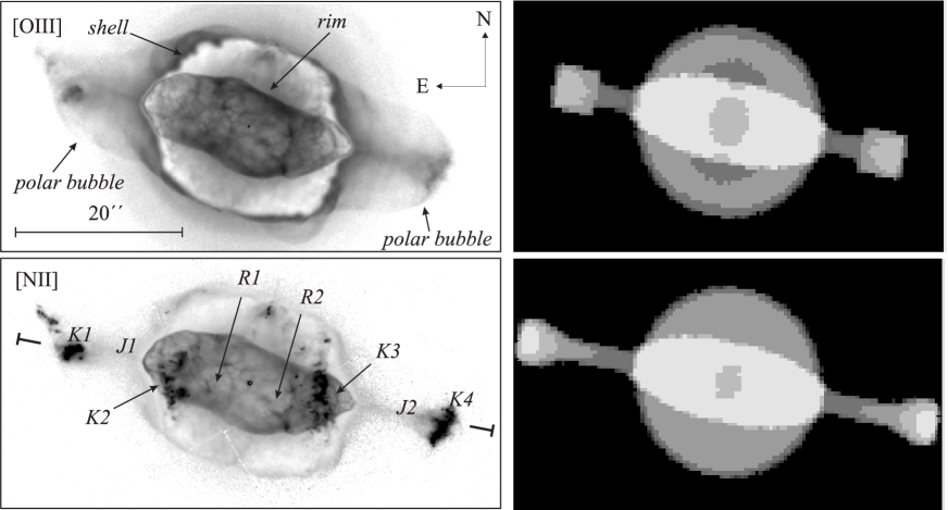
Figure 2: Left panel: HST [O iii] and [N ii] images of NGC 7009 on a logarithmic intensity scale; slit position for the spectra discussed in Section 3 is indicated by short lines (P.A. = 79^∘), while labels mark the position of the several structures, where “K”, “J” and “R” stand for “knot”, “jet”, and “rim”, respectively. Right panel: project emission maps from the model; the top map is [O iii] and the bottom one is [N ii]; maps (in arbitrary units) are not on the same colour intensity scale.

As noted in previous sections, the ionisation structure of the model is strongly dependent on the input 3D density distribution. Because of that, here we also present the results obtained with a slightly different geometry, which we call the alternative model. The only difference in terms of input density distribution between our initial model and the alternative one is that in the latter the jets start 3.3% further away from the central star than in the previous model. Since the H number density in the jet is four times lower than the value in the rim at the position of the polar axis, our change results into an increase in the line optical depth along the path connecting the central star to the outer pair of knots. The intensity of the ionizing stellar field reaching the knots is therefore decreased in our alternative model, hence resulting in a lower ionization level. Other model parameters were also adjusted in order to optimise our fit of the spectrum and these are summarised in Table 6. More importantly, with this alternative model we aimed at reproducing the more extreme [N ii] emission of the Eastern knot of the nebula ($\rm{Knot1}$ in Paper i and in Figure 2).

Table 6: Input parameters for the alternative model.

L∗ ($L_{\odot}$)	3136	N/H	2.8$\times$10-4
Teff (K)	82,000	O/H	4.5$\times$10-4
Rin (cm)	0.0	Ne/H	1.0$\times$10-4
Rout (cm)	3.88$\times$1017	S/H	0.9$\times$10-5
He/H	0.12	Ar/H	1.5$\times$10-6
C/H	3.5$\times$10-4	Fe/H	1.25$\times$10-6

Abundances are given by number, relative to H.

Table 7: Alternative model and observed dereddened spectra of R, K and NEB. Line intensities are normalized to H$\beta$=100.

Line Identification (Å)	R			K			NEB
	Model	Model	Obs.	Model	Model	Obs.	Model	Model	Obs.
	no-slit	slit		no-slit	slit		no-slit	slit
H$\beta$(10-13 erg cm-2 s-1)	3120	398.5	-	7.95	2.95	-	3137	407.1	3197*
[Oii] 3726.0 + 3728.8	5.37	5.95	15.5	257.	299.	204.	6.18	8.81	24.2
			7.34			155.
[Neiii] 3868.7	109.	110.	106.	123.	122.	82.3	109.	110.	108.
			105.			141.
**[Neiii] 3967.5	33.8	34.0	51.7	38.1	37.9	35.3	33.8	34.1	48.9
			44.6			59.8
[Sii] 4068.6	0.32	0.36	1.50	5.89	6.72	7.43	0.33	0.42	1.98
			2.36			5.04
[Sii] 4076.4	0.10	0.12	0.87	1.95	2.22	2.36	0.11	0.14	1.11
			1.16			1.83
[Oiii] 4363.2	9.11	9.13	7.76	9.86	9.39	6.94	9.12	9.16	8.15
			8.65			9.64
Heii 4685.7	18.4	24.0	26.0	0.00	0.00	1.00	18.3	23.5	15.8
			23.4			1.23
**[Ariv] 4711	4.28	4.23	5.48	1.49	1.38	2.19	4.27	4.19	4.10
			4.96			2.00
[Ariv] 4740.2	5.67	5.73	5.56	1.26	1.17	1.14	5.65	5.65	3.92
			4.54			1.49
H$\beta$ 4861.3	100.	100.	100.	100.	100.	100.	100.	100.	100.
			100.			100.
[Oiii] 5006.8	1234	1208	1162	1262	1205	1238	1234	1212	1206
			1225			1310
[Cliii] 5517.7	0.35	0.36	0.43	1.07	1.05	0.00	0.35	0.37	0.54
			0.43			0.97
[Cliii] 5537.9	0.57	0.59	0.53	1.03	1.01	0.00	0.57	0.60	0.64
			0.55			0.90
[Nii] 5754.6	0.15	0.16	0.14	5.33	6.32	6.49	0.16	0.22	0.46
			0.18			3.91
Hei 5875.7	15.0	14.3	13.9	17.0	17.0	18.8	15.0	14.4	14.5
			14.1			15.0
[Siii] 6312.1	1.50	1.57	1.27	3.97	3.91	3.89	1.50	1.61	1.68
			1.14			3.25
[Nii] 6583.4	8.12	9.32	7.09	296.	352.	355.	9.03	12.5	27.
			5.60			194.
Hei 6678.1	4.25	4.06	3.87	4.81	4.82	7.49	4.26	4.08	3.97
			3.95			3.18
[Sii] 6716.5	0.45	0.54	0.48	26.0	29.8	36.8	0.54	0.85	2.33
			0.38			23.2
[Sii] 6730.8	0.84	1.00	0.84	34.9	39.9	51.0	0.96	1.41	3.85
			0.69			28.4

As in Table 2, with the top/bottom rows given intensities of the Eastern/Western size of the nebula.

Table 8: Averaged fractional ionic abundances for the alternative model.

				Ion
Element	i	ii	iii	iv	v	vi	vii
H	5.53(-4)	0.999
	1.38(-2)	0.986
	6.91(-4)	0.999
He	6.95(-4)	0.809	0.190
	8.99(-3)	0.991
	7.83(-4)	0.813	0.186
C	3.19(-6)	1.06(-2)	0.542	0.440	6.48(-3)
	3.27(-4)	0.155	0.817	2.65(-2)
	6.13(-6)	1.21(-2)	0.547	0.433	6.35(-3)
N	1.39(-6)	5.70(-3)	0.533	0.455	5.08(-3)	1.62(-5)
	6.83(-4)	0.176	0.789	3.31(-2)
	6.86(-6)	7.34(-3)	0.539	0.448	4.972(-3)	1.58(-5)
O	4.90(-6)	9.40(-3)	0.856	0.130	3.94(-3)	1.95(-6)
	5.29(-3)	0.235	0.759
	4.68(-6)	1.15(-2)	0.856	0.127	3.85(-3)	1.90(-6)
Ne	3.42(-6)	1.02(-2)	0.910	7.85(-2)	1.03(-3)
	2.09(-4)	7.17(-2)	0.928
	5.27(-6)	1.09(-2)	0.911	7.69(-2)	1.00(-3)
S	7.12(-7)	8.03(-3)	0.333	0.548	0.105	3.38(-3)	1.58(-5)
	1.13(-4)	0.190	0.734	7.43(-2)	5.21(-4)
	1.72(-6)	9.94(-3)	0.340	0.542	0.103	3.31(-3)	1.55(-5)
Ar	1.54(-7)	1.22(-3)	0.351	0.621	2.17(-2)	3.94(-3)	4.39(-5)
	5.51(-5)	2.74(-2)	0.825	0.147
	6.02(-7)	1.48(-3)	0.358	0.614	2.12(-2)	3.86(-3)	4.30(-5)

Top to bottom rows give values for R, K and NEB, respectively.

As in the case of our original model discussed in Section 3, we found a good agreement of the alternative model with the dereddened fluxes of Paper i, for the rim, the knots as well as for the whole nebula (NEB). Again, most of the line intensities are within 10-30% of one of the sides of NGC 7009, or between the two values of the Eastern and Western sides, as quoted in Table 7, with the exceptions of the [S ii]$\lambda\lambda$4068,4076 and [S ii]$\lambda\lambda$6717,6731 doublets, as pointed out in Section 3.2.

The mean T_e of the alternative model also compare very nicely with the observed values, namely, T_e[O iii] and T_e[N ii] of 10,200 K and 9,950 K, 10,600 K and 10,600 K, and 10,200 K and 10,100 K, for rim, knots and NEB, respectively. And the N_e are automatically matched with the empirical values, since they are constraining the model as input parameters.

The corresponding ionisation structure is shown in Table 8, from which we obtain the N/N⁺ and O/O⁺ ratios of the different zones in the nebula, as being: 1.64 (R-component), 1.33 (K-component) and 1.56 (NEB), that, as above, are in contradiction with the ratios adopted in the empirical icf scheme. We chose to include Table 8 in the paper, although qualitatively similar to Table 5, to allow for model icfs to be derived at a later time should one wish to do so.

Finally, the projected emission maps obtained from this model are not shown here as they are qualitatively identical to those of our original model (right panels of Figure 2).

5 Conclusions

This work focused on the study of the apparent N overabundance in the outer knots of NGC 7009 with respect to the main nebular rim and shell.

Alexander & Balick (1997) and Gruenwald & Viegas (1998) showed that long-slit data may give spurious overabundances of N and other elements in the outer regions of model PNe. These authors have identified the different charge-exchange reaction rates of N and O as the main responsible for the effect in the low-ionization regions of the nebulae, therefore affecting the (N⁺/N)/(O⁺/O) ratio, that as discussed in Section 3.4, is commonly used to obtain the icf for nitrogen. However, as shown by Mampaso (2004) charge-exchange reactions can, in this case, account at most by 20% of the nitrogen overabundance of the knots of NGC 7009.

In this paper we have presented a model that was able to reproduce the main spectroscopic characteristics of the various spatial regions of NGC 7009 without the need of assuming an inhomogeneous set of abundances. We investigated the importance of taking into account the effects of a narrow slit, and our results in Table 3 and 7 show that the convolution of the model results with the profile of the narrow slit used for the observations presented in Paper i results in the [N ii] emission being enhanced respect to H$\beta$ in all regions of the nebula, with the effect being slightly more pronounced in the knots.

The (N⁺/N)/(O⁺/O) predicted by our models are 0.60, 0.72 and 0.62 (or alternatively, 0.61, 0.75 and 0.64) for the rim, knots and the whole nebula, respectively, all at variance with the icf assumption of unity for this ratio. The icfs will therefore be underestimated by the empirical scheme, both in the case of the R and K components, but more so in the former (by a factor of 1.21). Therefore this effect may partly be responsible for the apparent inhomogeneous N abundance derived from observations. The differences in the (N⁺/N)/(O⁺/O) in these two components may be due to a number of effects, including charge exchange, as stated above, and the difference in the ionization potentials of the relevant species, which makes the (N⁺/N)/(O⁺/O) ratio extremely sensitive to the shape of the local radiation field. For this reason, a realistic density distribution is essential to the modelling of a non-spherical object, if useful information is to be extracted from spatially resolved observations. The density distribution of the gas modifies the shape of the local radiation field via the gas opacities and (as demonstrated in Section 3.4 and Section 4) matching the emission line spectrum of a given nebular region relies, among other things, on the careful construction of a model capable of providing the correct optical depths in various directions.

Our main conclusions discussed here may also be extended to other PNe exhibiting FLIERs, such as NGC 6543 and NGC 6826, for which similar apparent chemical inhomogeneities have been claimed (Balick et al., 1994).

References

- Acker et al. (1992) Acker A., Ochsenbein, F. Stenholm, B., Tylenda R., Marcout J., & Schohn C., 1992, Strasbourg-ESO catalogue of Galactic planetary nebulae, ESO
- Alexander & Balick (1997) Alexander J., & Balick B., 1997, AJ, 114, 713
- Baker (1983) Baker T., 1983, ApJ, 267, 630
- Balick et al. (1987) Balick B., Preston H. L, & Icke V., 1987, AJ, 94, 164
- Balick et al. (1993) Balick B., Rugers M., Terzian Y., Chengalur J. N., 1993, ApJ, 411, 778
- Balick et al. (1994) Balick B., Perinotto M., Maccioni A., Alexander J., Terzian Y., & Hajian A. R., 1994, ApJ, 424, 800
- Balick et al (2001) Balick B., Wilson J., & Hajian A.R., 2001, AJ, 121, 354
- Cardelli et al. (1989) Cardelli J. A., Clayton G. C., & Mathis J. S., 1989, ApJ, 345, 245
- Corradi et al. (2004) Corradi R. L. M., Sánchez-Blázquez P., Mellema G., Giammanco C., & Schwarz H. E., 2004, A&A, 417, 637
- Ercolano et al. (2003a) Ercolano B., Barlow M. J., Storey P. J., & Liu X.-W. 2003a, MNRAS, 340, 1136
- Ercolano et al. (2003b) Ercolano B., Morisset C., Barlow M. J., Storey P. J., & Liu X.-W. 2003b, MNRAS, 340, 1153
- Ercolano et al. (2003c) Ercolano B., Barlow M. J., Storey P. J., & Liu X.-W., Rauch T., Werner K., 2003c, MNRAS, 344, 1145
- Ercolano et al. (2004) Ercolano B., Wesson R., Zhang Y., Barlow M. J., De Marco O., Rauch T., Liu X.-W., 2004, MNRAS, 354, 558
- Fernández et al. (2004) Fernández R., Monteiro H., & Schwarz H. E., 2004, ApJ, 603, 595
- Garay et al. (1989) Garay G., Gathier R., Rodriguez L. F., 1989, A&A, 215,101
- Gonçalves et al. (2001) Gonçalves D. R., Corradi R. L. M., & Mampaso A., 2001, ApJ, 547, 302
- Gonçalves et al. (2003) Gonçalves D. R., Corradi R. L. M., Mampaso A., & Perinotto M., 2003, ApJ, 597, 975
- Gonçalves (2004) Gonçalves D. R., 2004, in Asymmetrical Planetary Nebulae III: Winds, Structure and the Thunderbird, Edited by Margaret Meixner, Joel H. Kastner, Bruce Balick and Noam Soker. ASP Conference Proceedings, Vol. 313, p. 216
- Gonçalves et al. (2004) Gonçalves D. R., Mampaso A., Corradi R. L. M., Perinotto M., Riera A., López-Martín L., 2004, MNRAS, 355, 37
- Gruenwald & Viegas (1998) Gruenwald R., & Viegas S. M., 1998, ApJ, 501, 221
- Hajian et al. (1997) Hajian A. R., Balick B., Terzian Y., & Perinotto M., 1997, ApJ, 304, 313
- Hyung & Aller (1995a) Hyung S., & Aller L. H, 1995, MNRAS, 273, 958
- Hyung & Aller (1995b) Hyung S., & Aller L. H, 1995, MNRAS, 273, 973
- Kingsburgh & Barlow (1992) Kingsburgh, R. L. & Barlow M. J., 1992, MNRAS, 257, 317
- Kingsburgh & Barlow (1994) Kingsburgh, R. L. & Barlow M. J., 1994, MNRAS, 271, 257
- Kwitter & Henry (1998) Kwitter K. B., & Henry R. B., 1998, ApJ, 493, 247
- Liu et al. (1995) Liu, X.-W., Storey, P. J., Barlow, M. J., Clegg, R. E. S., 1995, MNRAS, 272, 369
- López et al. (1995) López, J. A. , Vázquez, R., Rodríguez, L. F., 1995, ApJL, 455, L63
- Luo et al. (2001) Luo S.-G., Liu X.-W., & Barlow M. J., 2001, MNRAS, 326, 1049
- Mampaso (2004) Mampaso A., 2004, in Asymmetrical Planetary Nebulae III: Winds, Structure and the Thunderbird, Edited by Margaret Meixner, Joel H. Kastner, Bruce Balick and Noam Soker. ASP Conference Proceedings, Vol. 313, p. 265
- Mathis et al. (1998) Mathis J. S., Torres-Peimbert S., Peimbert M., 1998 ApJ, 495, 328
- Méndez et al. (1992) Méndez R. H., Kudritzki R. P., & Herrero A., 1992, A&A, 260, 329
- Moreno et al. (1998) Moreno M.A., de la Fuente E., & Gutiérrez F., 1998, RevMxAA, 34, 117
- Perinotto et al. (2004a) Perinotto M., Patriarchi P., Balick B., Corradi R. L. M., 2004a, A&A, 422, 963
- Perinotto et al. (2004b) Perinotto M., Patriarchi P., Morbidelli L., & Scatarzi A., 2004b, MNRAS, 349, 793
- Péquignot et al. (2001) Péquignot, D., Ferland, G., Netzer, H., Kallman, T., Ballantyne, D., Dumont, A.-M., Ercolano, B., Harrington, P., Kraemer, S., Morisset, C., Nayakshin, S., Rubin, R. H. and Sutherland, R., 2001, Spectroscopic Challenges of Photoionized Plasmas, ASP Conference Series, 247, 533
- Pottasch (2000) Pottasch S. R., 2000, in Asymmetrical Planetary Nebulae II: From Origins to Microstructures, ASP Conference Series, Vol. 199., Edited by J. H. Kastner, N. Soker, and S. Rappaport, p. 289
- Reay & Atherton (1985) Reay N. K., & Atherton P.D., 1985, MNRAS, 215, 233
- Rubin et al. (2002) Rubin R. H., et al., 2002, MNRAS, 334, 777
- Sabbadin et al. (2004) Sabbadin F., Turatto M., Cappellaro E., Benetti S. & Ragazzoni R., 2004, A&A, 416, 955
- Stasińska (2004) Stasińska G., 2004, In Cosmochemistry. The melting pot of the elements. XIII Canary Islands Winter School of Astrophysics, edited by C. Esteban, R. J. García-López, A. Herrero, F. Sánchez. Cambridge, UK: Cambridge University Press, p. 115