1.0

Tracing the first stars with cosmic infrared background fluctuations

The deepest space and ground-based observations find metal-enriched galaxies at cosmic times when the Universe was $<1$ Gyr old. These stellar populations had to be preceded by the metal-free first stars, Population III. Recent cosmic microwave background polarization measurements indicate that stars started forming early when the Universe was ${{}_{<}\atop{}^{\sim}}200$ Myr old. Theoretically it is now thought that Population III stars were significantly more massive than the present metal-rich stellar populations. While such sources will not be individually detectable by existing or planned telescopes, they would have produced significant cosmic infrared background radiation in the near-infrared, whose fluctuations reflect the conditions in the primordial density field. Here we report a measurement of diffuse flux fluctuations after removing foreground stars and galaxies. The anisotropies exceed the instrument noise and the more local foregrounds and can be attributed to emission from massive Population III stars, providing observational evidence of an era dominated by these objects.

The cosmic infrared background (CIB) is generated by emission from luminous objects during the entire history of the Universe including epochs at which discrete objects are inaccessible to current telescopic studies [1, 2]. With new powerful telescopes individual galaxies are now found out to redshifts of $z{{}_{>}\atop{}^{\sim}}5-7$, but the period preceding that of the galaxies seen in the Hubble Ultra-Deep Field (UDF) remains largely unexplored. The UDF galaxies and even the highest $z$ quasars ($z{{}_{>}\atop{}^{\sim}}6.5$) appear to consist of “ordinary” metal-enriched Population I and II stars, suggesting that the metal-free stars of Population III lived at still earlier epochs. Large-scale polarization of the cosmic microwave background (CMB) [3] suggests that first stars formed early at $z\sim 20$.

Current theory predicts that Population III objects were very massive stars with mass $>100M_{\odot}$ [5, 6, 37]. They should have produced a significant diffuse background [7] with an intensity almost independent of the details of their mass function [13]. Because much of the emission longward of the rest-frame Lyman limit from these epochs is now shifted into the near-IR (NIR), these stars could be responsible for producing much, or all, of the observed NIR CIB excess over that from normal galaxy populations (see detailed review in [2] and refs. [8, 9, 10, 11, 12, 13]). Two groups [12, 13] have recently suggested that this emission should have a distinct angular spectrum of anisotropies, which can be measured if the contributions from the ordinary (metal-rich) galaxies and foregrounds can be isolated and removed, and provide an indication of the era made predominantly of the massive Populations III stars.

Measuring CIB anisotropies from objects at high $z$ is difficult because the spatial fluctuations are small and can be hidden by the contributions of ordinary low-$z$ galaxies as well as instrument noise and systematic errors in the data. Previous attempts to measure the structure of the CIB in the near–IR on the degree scale with COBE/DIRBE [21], IRTS/NIRS [29] were limited in sensitivity because of the remaining contributions from brighter galaxies in the large beams. Analysis of 2MASS data at 1.25, 1.65 and 2.2 $\mu$m with $\sim 2$ arcsec resolution [33, 34] allowed removal of foreground galaxies to a K magnitude of 19-19.5 ($m_{AB}\sim 21$ or 15 $\mu$Jy) and led to measurements of CIB fluctuations at 1.25 to 2.2 $\mu$m  at sub-arcminute angular scales. These studies reported fluctuations in excess of that expected from the observed galaxy populations, although their accurate interpretation in terms of high-$z$ contributions is difficult due to foreground galaxies and non-optimal angular scales.

We used data from deep exposure data obtained with Spitzer/IRAC [15, 19] in four channels (Channels 1-4 correspond to wavelengths of 3.6, 4.5, 5.8 and 8 $\mu$m respectively) in attempting to uncover this signal. We find significant CIB anisotropies after subtracting galaxies substantially fainter than was possible in prior studies, i.e. down to $m_{\rm AB}\sim 22-25$. The angular power spectrum of the anisotropies is significantly different from that expected from Solar System and Galactic sources, its amplitude is much larger than what is expected from the remaining faint galaxies, and can reasonably be attributed to the diffuse light from the Population III era.

Assembly and reduction of data sets. The primary data set used here is the deep IRAC observation of a $\sim 12{{}^{\prime}}\times 6{{}^{\prime}}$ region around QSO HS 1700+6416 obtained by the Spitzer instrument team [14, 15]. In addition, the data from two auxiliary fields with shallower exposures (HZF and EGS) were analyzed. Relevant data characterising the fields are listed in Table 1. For this analysis the raw data were reduced using a least-squares self-calibration method [18]; the processing is described in more detail in the Supplementary Information (hereafter SI).

Table 1: Analyzed fields, their coordinates, exposure times, limiting magnitudes, and pixel scales

Region	QSO 1700 (Ch 1-4)	HZF (Ch 1-3)	HZF (Ch 4)	EGS (Ch 1-4)
$(\alpha,\delta)$	(255.3, 64.2)	(136.0, 11.6)	(285.7, $-17.6$)	(215.5, 53.3)
$(l,b)_{\rm Gal}$	(94.4, 36.1)	(217.5, 34.6)	(18.4, $-10.4$)	(96.5, 58.9)
$(\lambda,\beta)_{\rm Ecl}$	(194.3, 83.5)	(135.0, $-4.9$)	(285.0, 5.0)	(179.9, 60.9)
$\langle t_{\rm obs}\rangle(hrs)$	7.8, 7.8, 7.8, 9.2	0.5, 0.5, 0.5	0.7	1.4, 1.4, 1.4, 1.4
$m_{\rm Vega,lim}$	22.5, 20.5, 18.25, 17.5	21.5, 19.5, 17	14.5	22.5, 20.75, 18.5, 17.75
Pixel scale (′′)	0.6	1.2	1.2	1.2
Field size (pix)	$1,152\times 512$	$576\times 256$	$576\times 256$	$640\times 384$

QSO 1700 was observed during In-Orbit Checkout (IOC) with eight AORs (Astronomical Observation Requests) which used various dither patterns and 200-sec frame times, except for two which used 100-sec frame times (AOR ID numbers = 7127552, 7127808, 7128064, 7128320, 7128576, 7475968, 7476224, 7476480). Because of the focal plane offset between the shared 3.6/5.8 ${\mu{\rm m}}$ and 4.5/8 ${\mu{\rm m}}$ fields of view, each of these pairs observes separate fields which have a common overlap of $\sim 5{{}^{\prime}}\times 5{{}^{\prime}}$ at all four wavelengths. To provide contrast for the self-calibration algorithm, data from a high-zodiacal light brightness field (HZF) was co-processed for each channel. For 3.6, 4.5, and 5.8 ${\mu{\rm m}}$, the nearest suitable (200-second frame time) data were observed later during IOC (AORID number = 8080896). For the 8 ${\mu{\rm m}}$ data, because nominal 100 and 200-second frame times are split into pairs and quartets of 50-second frames, more nearly contemporaneous observations earlier during IOC were used (AORID number = 6849280). For this work we only self-calibrated the six 200-second AORs for 3.6 - 5.8 ${\mu{\rm m}}$, but at 8 ${\mu{\rm m}}$ all eight AORs were used since all produce data with 50-second frame times. Observations of the extended Groth Strip area (EGS) provide an additional deep data set for verification of our results. Separate exposure times and limiting magnitudes apply for Channels 1 - 4 respectively. The maps for the main QSO 1700 field are shown in SI (the supplementary information available at Nature online).

The random noise level of the maps was computed from two subsets (A, B) containing the odd and even numbered frames, respectively, of the observing sequence. The A and B subsets were observed nearly simultaneously and with similar dither patterns and exposures. The difference between maps generated from the A and B subsets should eliminate true celestial sources and stable instrumental effects and reflect only the random noise of the observations.

Analysis of the background fluctuations must be preceded by steps that eliminate the foreground Galactic stars and the galaxies bright enough to be individually resolved. The primary means of removing these sources is an iterative clipping algorithm which zeros all pixels (and a fixed number of neighboring pixels, $N_{\rm mask}\times N_{\rm mask}$) which are more than a chosen factor, $N_{\rm cut}$, above the 1$\sigma$ RMS variation in the clipped surface brightness. This must be restricted to relatively high $N_{\rm cut}$ to (a) leave enough area for a robust Fourier analysis of the map, and (b) avoid clipping into the background fluctuation distribution. This means that faint sources, the faint outer portions of resolved galaxies, and the faint wings of the point source response function around bright stars cannot be clipped adequately. To remove these low surface brightness sources we used a CLEAN algorithm [16] to model the entire field in each channel. This model, convolved with the full IRAC point spread function (PSF), was subtracted from the unclipped regions of the map. SI provides details on this process and illustrations of the clipped and model-subtracted images. The final step is the fitting and removal of the 0th and 1st order components of the background in the unclipped regions. This is done to minimize power spectrum artifacts due to the clipping, and because the lack of an absolute flux reference measurement and observing constraints prohibit unambiguous determination of these components. With this subtraction, the images represent the fluctuation fields, $\delta F($$x$), rather than the absolute intensity. For each observed field these steps were carried out for images derived from the full data set and from the A and B subsets.

Power spectrum computation and analysis. For each channel, we calculate the power spectra of the fluctuations as a quantitative means of characterizing their scale and amplitude. The power that remains after subtraction of the random noise component is insensitive to the details of the source clipping, and is statistically correlated between channels. This confirms that the fluctuation signal does have a celestial origin. The shape and amplitude of the power spectra are not consistent with significant contributions from the cirrus of the interstellar medium (except perhaps at 8$\mu$m) or from the zodiacal light from local interplanetary dust.

The fluctuation field, $\delta F($$x$), was weighted by the observation time in each pixel, $w($$x$$)\propto t_{\rm obs}($$x$), and its Fourier transform, $f($$q$$)=\int\delta F($$x$$)w($$x$$)\exp(-i$$x$$\cdot$$q$$)d^{2}x$ calculated using the fast Fourier transform. (The weighting is necessary to minimize the noise variations across the image, but we also performed the same analysis without it and verified that the weight adds no structure to the resultant power spectrum. This is because the weights are relatively flat across the image). The power spectrum is $P_{2}(q)=\langle|f($$q$$)|^{2}\rangle$, with the average taken over all the Fourier elements $N_{q}$ corresponding to the given $q$. A typical flux fluctuation is $\sqrt{q^{2}P_{2}(q)/2\pi}$ on the angular scale of wavelength $2\pi/q$. In SI we show the final power spectrum of the diffuse flux fluctuations, $P_{S}(q)$, and the noise, $P_{N}(q)$, of the datasets. We find significant excess of the large-scale fluctuations over the instrument noise.

Fig. 1 shows the excess power spectrum, $P_{S}(q)-P_{N}(q)$, of the diffuse light after the instrument noise has been subtracted. There is a clear positive residual whose power spectrum is significantly different from white noise and has substantial correlations all the way to the largest scales probed. Possible sources of these large-scale correlations can be artifacts of the analysis procedure (e.g. clipping and FFT), instrumental artifacts, local Solar System or Galactic emission, or relatively nearby extragalactic sources and/or more distant cosmological sources. In what follows we discuss their relative contributions.

Residual emission from the wings of incompletely clipped sources can give rise to spurious fluctuations, but the power spectrum of these fluctuations should depend on the clipping parameters $N_{\rm cut}$ and $N_{\rm mask}$. We tested the contributions from these residuals in various ways. For a given $N_{\rm cut}$ we varied $N_{\rm mask}$ from 3 to 7 significantly reducing any residual wings and increasing the fraction of the clipped pixels, but found negligible (${{}_{<}\atop{}^{\sim}}$ a few percent) variations in the final $P_{2}(q)$. We also clipped down to progressively lower values of $N_{\rm cut}$. For $N_{\rm cut}{{}_{<}\atop{}^{\sim}}3.5$ too few pixels remain for robust Fourier analysis, so in these cases we computed $C(\theta)$, the correlation function of the diffuse emission, related to the power spectrum by a 1-D Legendre transformation. It is consistent with the fluctuations in Fig. 1 as discussed and shown in SI.

Instrument noise contributions to the fluctuations were evaluated as the power spectra of $\frac{1}{2}(\delta F_{A}-\delta F_{B})$ using the $A-B$ subset images. As shown in SI, random instrument noise has an approximately white spectrum. The power spectra of the final datasets have a much larger amplitude than the noise (especially in Channels 1 and 2) until the convolution with the beam tapers off the signals from the sky at the smallest angular scales. The instrument noise spectra are unaffected by the beam and are uncorrelated from channel to channel, as expected. However, the full data set fluctuation fields show statistically significant correlations between channels as shown in Table 2. This means that we see the same fluctuation field in addition to (different) noise in all four channels. SI describes tests to assess the contributions of possible instrumental systematic errors. They indicate that systematic instrumental effects are unlikely to lead to the signal shown in Fig. 1.

Table 2: Cross-correlation of fluctuations in units of that of random sample ${\cal R}/\sigma_{\cal R}$ for various clipping thresholds

Channels	$N_{\rm cut}$ = 4	$N_{\rm cut}$ = 2
1 : 2	52	12
1 : 3	7	0.6
1 : 4	10	4

These correlations were evaluated for an evenly covered region of $512^{2}$ pixels common to all 4 channels for the QSO 1700 field. For random uncorrelated samples, $\delta_{1},\delta_{2}$, of $N_{\rm pixels}$ the correlation coefficient, ${\cal R}\equiv\langle\delta_{1}\delta_{2}\rangle/[\langle\delta_{1}^{2}\rangle\langle\delta_{2}^{2}\rangle]^{1/2}$, should be zero with dispersion $\sigma_{\cal R}=N_{\rm pixels}^{-1/2}$. Whereas, for $N_{\rm mask}=3$, we find that down to even $N_{\rm cut}=2$, when only 6% of the pixels remain, the correlations between the channels remain statistically significant. Simple simulations containing the appropriate levels of the instrument noise and a power law component of the CIB gave somewhat larger mean values of ${\cal R}$ with the measured values lying within a 95% confidence level; incorporating the possibility that not all of the remaining ordinary galaxies are the same at each wavelength would however reduce the mean values of ${\cal R}$.

The best assessment of zodiacal light contributions to the power spectrum comes from the examination of EGS observations taken at two epochs 6 months apart. Because any anisotropies in the zodiacal light cloud will not remain fixed in celestial coordinates over this interval, the difference in the fluctuation fields at these two epochs should eliminate Galactic and extragalactic signals and yield a power spectrum of the zodiacal light fluctuations added to the instrument noise and possible systematic errors. The fluctuation levels of these difference maps set an upper limit on the zodiacal light contribution of $<0.1$ $\rm nW/m^{2}/sr\$at 8 $\mu$m. Scaling this result to the other channels by interpolating the observed zodiacal light spectrum [36] leads to zodiacal light contributions to the fluctuations that are comfortably below the detections in Fig. 1 in the other channels as well.

Our assessment of the contribution of the infrared cirrus (i.e. interstellar clouds of neutral gas and dust) to the power spectra is derived from the 8 $\mu$m HZF field which lies at low $b_{\rm Gal}$ and is visibly contaminated by cirrus. Assuming that the large scale fluctuations in this field are due to the cirrus, relative fluctuations of the 8 $\mu$m cirrus are $\sim 1$% of the mean cirrus flux level. A similar level of relative cirrus fluctuations in the QSO 1700 field would have an amplitude of $\sim 0.3$ nW/m²/sr. This is not significantly lower than the 8 $\mu$m amplitude observed in Fig. 1. Therefore, we cannot presently eliminate the possibility that the fluctuations at 8 $\mu$m are dominated by cirrus. However, the spectrum of the ISM emission should drop sharply at shorter wavelengths as the PAH emission bands that dominate at 8 $\mu$m become less significant. Given this estimate of the cirrus contribution at 8 $\mu$m we estimate the amplitude of large-scale fluctuations for channels 1 – 3 as $\simeq$ 0.03, 0.03, and 0.08 nW/m²/sr, which are well below the observed fluctuations in these channels.

Colour is another important criterion for testing the origins of the signal in Fig. 1. The cross-correlations between the channels for the common area of the QSO 1700 field are statistically significant and they also strengthen at the larger scales where the noise contribution is smaller, as verified by smoothing the maps. These significant cross-correlations allow us to examine the corresponding colours of the fluctuations. We made several estimates of the colours, $\beta_{n1}$, between channels $n$ and 1: a) as the square root of ratio of the power spectra, and b) as $\beta_{n1}(\theta)=\langle\delta_{n}(x)\delta_{1}(x+\theta)\rangle/\langle\delta_{1}(x)\delta_{1}(x+\theta)\rangle$ evaluated over the 512² pixel field common to all four channels, where a further consistency check comes from comparison between $\beta_{21}$ and $\beta_{41}/\beta_{42}$. For channels 1 and 2 these estimates are shown in Fig. 2 and appear roughly independent of angular scale and mutually consistent. The instrument noise is too large to enable robust colour estimates involving channel 3 (5.8 $\mu$m). These derived colours indicate that the fluctuation signal in Fig. 1 has an energy distribution that is approximately flat to slowly rising with wavelength in $\nu I_{\nu}$. The energy spectrum rules out contributions from remaining Galactic stars, but probably cannot be used to distinguish between ordinary galaxies and Pop III objects without additional detailed modeling of both sets of sources.

CIB fluctuations from extragalactic sources. There are two extragalactic classes of contributors to CIB fluctuations: “ordinary” galaxies containing normal stellar Populations I and II, and the objects that preceded them, Population III stars. The square of the CIB fluctuation in band $\nu$ produced by cosmological sources that existed over time period $\Delta t$ is given by the power-spectrum version of the Limber equation (see [2] and SI):

$$\frac{q^{2}P_{2}(q)}{2\pi}=\Delta t\int\left(\frac{dI_{\nu^{\prime}}}{dt}\right)^{2}\Delta^{2}(qd_{A}^{-1};z)dt$$ (1)

where $\nu^{\prime}=\nu(1+z)$ is the rest frequency of the emitters, $d_{A}$ is the comoving angular diameter distance and

$$\Delta(k)=\sqrt{\frac{1}{2\pi}\frac{k^{2}P_{3}(k)}{c\Delta t}}$$ (2)

is the fluctuation in the number of sources within a volume $k^{-2}c\Delta t$. The fluctuation of the CIB on angular scale $\simeq 2\pi/q$ can then be expressed as $\delta F_{\rm CIB}=F_{\rm CIB}\Delta(qd_{A}^{-1}(\langle z\rangle))$, where $\langle z\rangle$ is the suitably averaged effective redshift. The relative CIB fluctuation is a suitably averaged fluctuation in the source counts over a cylinder of radius $q^{-1}d_{A}(\langle z\rangle)$ and length $c\Delta t$. Three things would lead to larger fluctuations: 1) a population that, after removing constituents brighter than some limit, leaves a substantial mean CIB flux (increase $F_{\rm CIB}$), 2) populations that existed for a shorter time (increase $\langle\Delta\rangle$ by decreasing $\Delta t$), and 3) populations that formed out of rare peaks of the underlying density field leading to biased and significantly amplified, [27] clustering properties (increase $\langle\Delta\rangle$ by increasing $P_{3}(k))$.

CIB fluctuations from remaining ordinary galaxies. The fluctuations produced by ordinary galaxies contain two components: 1) shot noise from discrete galaxies and 2) galaxy clustering from the primeval density field. The amplitude of the first component can be estimated directly from galaxy counts. In order to estimate the contribution from the second component we proceed as follows: from galaxy count data we estimate the total CIB flux produced by the remaining galaxies fainter than our clipping threshold. Ordinary galaxies occupy an era of $\Delta t{{}_{>}\atop{}^{\sim}}$ a few Gyrs. Their present-day clustering pattern on the relevant scales is well measured today. The clustering pattern evolution can be extrapolated to earlier times assuming the “concordance” $\Lambda$CDM model. These parameters (flux, $\Delta t$, clustering pattern and its evolution) then allow us to estimate the contribution to the CIB fluctuations via eqs. 1,2. Because galaxy clustering is weaker at earlier times, an upper limit on the contribution from ordinary galaxies is obtained assuming that the clustering at early times remained the same as at $z=0$.

The shot noise component contributed by the ordinary galaxies to the CIB angular spectrum was estimated directly from galaxy count data: each magnitude bin $\Delta m$ with galaxies of flux $f(m)$ would contribute a power spectrum of $P_{\rm sn}=f^{2}(m)\frac{dN_{\rm gal}}{dm}\Delta m$. Fig. 1 shows the shot noise component convolved with the IRAC beam for the galaxies at the limiting magnitude in Table 1. The limiting magnitudes are qualitative estimates of where the SExtractor [22] number counts (in 0.5 magnitude bins) begin to drop sharply due to incompleteness. The shot noise fits the observed diffuse light fluctuations well at small angles, but the shot-noise contribution from ordinary galaxies cannot make a substantial contribution to the large scale power of the diffuse light in Fig. 1.

We assume the “concordance” $\Lambda$CDM model Universe with flat geometry ($\Omega_{\rm total}$=1) dominated by a cosmological constant, $\Omega_{\Lambda}\simeq 0.7$, with the rest coming from cold dark matter and ordinary baryons in proportions suggested by measurements of the CMB anisotropies [4] and high-$z$ supernovae [47]. With $P_{3}(k)$ taken from the $\Lambda$CDM concordance model, the power in fluctuations from the clustering of ordinary galaxies depends on the net flux produced by the remaining ordinary galaxies (via $F_{\rm CIB}$) and their typical redshifts (via $\Delta(qd_{a}^{-1})$). The total flux from galaxies fainter than the limiting magnitude in Table 1 was estimated from the Spitzer IRAC galaxy counts ([15]) and is shown in Fig. 3. The flux contributed to the CIB from the remaining galaxies is between 0.1 and 0.2 $\rm nW/m^{2}/sr\$and this amplitude is much less than the excess CIB at these wavelengths ([2]) indicating that the excess CIB flux is produced by populations that are still farther out than the ordinary galaxies remaining in the data. This (low) value of the remaining flux can also be derived from the small amplitude of the residual shot-noise contribution to the fluctuations in the confusion-limited datasets. Thus, in order to explain the amplitudes shown in Fig. 1, the remaining ordinary galaxy populations would need to produce relative flux fluctuations of order ${{}_{>}\atop{}^{\sim}}100\%$ from their clustering. Without follow-up spectroscopy it is difficult to determine with high precision the range of redshifts of the remaining ordinary galaxies, but approximate estimates can be made and are summarized in the Figure 3 legend to be $z{{}_{>}\atop{}^{\sim}}1$.

In flat cosmology with $\Omega_{\Lambda}=0.7$ one arcminute subtends a comoving scale between 0.7 and 1.6 $h^{-1}$Mpc at $z$ between 1 and 5. The present day 3-D power spectrum of galaxy clustering, $P_{3,\rm gal}(k)$, is described well by the concordance $\Lambda$CDM model ([25], [26]) and one expects that on arcminute scales the density field was in the linear to quasi-linear regime at the redshifts probed by the remaining galaxies between 3.6 and 8 $\mu$m. At smaller scales non-linear corrections to evolution were computed following ([44]). The resultant CIB fluctuation from the remaining ordinary galaxies, producing $F_{\rm CIB,og}=0.14$ $\rm nW/m^{2}/sr\$, times $\Delta(\propto(\Delta t)^{-1/2})$ is shown in Fig. 1 for $\langle z\rangle$=1,3,5 and $\Delta t$=5 Gyr corresponding to the age of the Universe at $z\sim 1$. For the $\Lambda$CDM model the relative fluctuations in the CIB on arcminute scales would be of order $\langle\Delta\rangle\sim(2-10)\times 10^{-2}(\Delta t/{\rm 5Gyr})^{-0.5}$ from galaxies with $\langle z\rangle$=1-5 assuming no biasing. Combining this with the above values for the diffuse flux from the remaining ordinary galaxies would lead to $\delta F{{}_{<}\atop{}^{\sim}}(1-2)\times 10^{-2}$ $\rm nW/m^{2}/sr\$in all the channels. While biasing may increase the relative fluctuations, with reasonable bias factors for galaxies lying at $z\sim$ (a few), the diffuse light fluctuations would still be very small compared to those in Fig. 1 and are unlikely to account for fluctuations of amplitude $\sim(0.1-0.5)$ $\rm nW/m^{2}/sr\$at arcminute scales. An upper limit on the CIB fluctuations can be evaluated assuming the same clustering pattern for the remaining galaxies as at the present epoch, $z=0$, i.e. that their 2-point correlation function is given by $\xi=(r/r_{*})^{-1.7}$ with $r_{*}=5.5h^{-1}$Mpc [46]; its $\Delta$ times $F_{\rm CIB,og}$ is also shown in Fig.1 and is much below the signal we measure. Conversely, one can evaluate the clustering strength needed to account for the observed fluctuations: a 100% relative fluctuation from galaxies at $z{{}_{>}\atop{}^{\sim}}1$ clustered with $\xi=(r/r_{*})^{-1.7}$ would require $r_{*}{{}_{>}\atop{}^{\sim}}25h^{-1}$Mpc. This corresponds to the effective bias factor ${{}_{>}\atop{}^{\sim}}5$ which is significantly higher than expected from gravitational clustering evolution in the $\Lambda$CDM Universe [35]. In fact, direct measurements of clustering for relatively nearby IRAC galaxies with flux $>32\mu$Jy at 3.6 $\mu$m ($\sim$5 magnitudes brighter than the limit reached for remaining galaxies in the QSO 1700 field) [48] find the projected 2-point correlation amplitude on $\sim$arcmin scales of $w_{>32\mu{\rm Jy}}(\theta{{}_{>}\atop{}^{\sim}}1^{\prime})<4\times 10^{-2}$ corresponding to relative fluctuations in CIB from these galaxies of amplitude $\sim\sqrt{w}{{}_{<}\atop{}^{\sim}}0.2$. Fainter galaxies are expected to have an even lower correlation amplitude.

The QSO 1700 field seems to contain an overdensity of Lyman-break galaxies at $z\simeq 2.3$ [45], which could lead to a larger $\Delta$ and CIB fluctuations for this region. However, we see similar levels of fluctuations for the other fields located at very different parts of the sky making it unlikely that the overdensity claimed in ref. [45] can account for our signal. When account is made of the different shot noise levels from the remaining galaxies, the fluctuations seen in the different fields have consistent power spectra within the statistical uncertainties. (An exception being channel 4 HZF data, located at low $b_{\rm Gal}$, and clearly dominated by Galactic cirrus).

CIB fluctuations from the Population III era. Population III at $z\sim$10-30 are expected to precede ordinary galaxy populations. One can expect on fairly general grounds [13] that, if massive, they would contribute significantly to the NIR CIB, both its mean level and anisotropies. Intuitive reasons are discussed in [2], but as eqs. 1,2 shows they are mostly related to: 1) if massive, Population III were very efficient light emitters, 2) their era likely lasted a shorter time, $\Delta t$, than that of the ordinary galaxies, leading to larger $\Delta$ in eq.2, and 3) they should have formed out of high peaks of the density field whose correlation function is strongly amplified. The near-IR also probes UV to visible parts of the electromagnetic spectrum at $z\sim 10-30$, where most of their emission is produced [11].

The amplitude of the CIB anisotropies remaining in the present data implies that the remaining CIB originates from still fainter objects. Can the observed amplitudes of fluctuations in Fig. 1 be accounted for by energetic sources at high $z$? Population III stars can produce significant NIR CIB levels [11], ${{}_{>}\atop{}^{\sim}}1$ $\rm nW/m^{2}/sr\$and e.g. the NIR CIB excess over that from ordinary galaxies at 3.6 $\mu$m is $8.7\pm 3.1$ $\rm nW/m^{2}/sr\$[2]. Thus Population III objects would require smaller relative CIB fluctuations. Because individual Population III systems are small, yet numerous, the shot-noise component of the CIB from them is small and, in any case, is already absorbed in the shot-noise shown in Fig. 1. Additionally, their $\langle\Delta\rangle$ would be amplified by the much shorter $\Delta t$ and (significant) biasing, and Population III contribution would dominate the diffuse light fluctuations in Fig. 1. Detailed theoretical interpretation of the results in terms of the Population III era models exceeds the scope of this article, but qualitative comparison can be made by estimating the typical value of the relative CIB fluctuation, $\Delta$, corresponding to that era. The fraction of the Population III haloes was calculated assuming that they form from the $\Lambda$CDM density field in haloes where the virial temperature $T_{\rm vir}\geq 2000$ K to enable efficient molecular hydrogen cooling ([38]). Biasing was treated using the gravitational clustering prescription from [39] in the $\Lambda$CDM model. (Non-linear evolution effects are small on the angular scales and redshifts probed here.) Assuming $\Delta t$=300 Myr, which corresponds to the age of the Universe at $z$=10, we get typical values of $\Delta\simeq$ 0.1-0.2 at $z$ between 10 and 20. This order-of-magnitude evaluation shows that the levels of $\sim$0.1-0.3 $\rm nW/m^{2}/sr\$at 3.6 to 8 $\mu$m on arcminute scales can be accounted for by Population III emissions if their total flux contribution is $>1$ $\rm nW/m^{2}/sr\$which is reasonable as discussed earlier.

Earlier studies of CIB fluctuations [21],[33],[29] contained significant contributions from relatively bright galaxies making it difficult to isolate the possible CIB fluctuations from the very early times. The contribution to CIB fluctuations from remaining galaxies is a function of the limiting magnitude below which galaxies are removed. With the Spitzer IRAC data we could identify and remove galaxies to very faint limits of flux ${{}_{>}\atop{}^{\sim}}0.3\mu$Jy. This limit is, at last, sufficiently low to push the residual contribution from ordinary galaxies along the line-of-sight below the level of the excess signal at larger angular scales. If our interpretation is correct and the signal we detect comes from Population III located at much higher $z$, the amplitude of the CIB fluctuations on scales where galaxy shot-noise is negligible should remain the same as fainter ordinary galaxies are removed with deeper clipping. This is true as far as we can test with this data and would certainly be verifiable with longer exposure data.

At these $z$ the IRAC bands probe the rest-frame wavelengths between 0.2 and 0.8 $\mu$m, where the energy spectrum of individual Population III object is dominated by free-free emission and is a slowly rising function of wavelength [11]; this would be consistent with the spectrum of the CIB anisotropies in Fig. 1. Near-IR observations at shorter wavelengths would be particularly important in confirming the redshifts where the CIB fluctuations originate as there should be a significant drop in the fluctuations power at the rest-frame Lyman limit wavelength.

Acknowledgements We thank Giovanni Fazio for access to the IRAC Deep Survey data and Dale Fixsen and Gary Hinshaw for comments on drafts of this paper. This material is based upon work supported by the National Science Foundation. This work is based on observations made with the Spitzer Space Telescope, which is operated by the Jet Propulsion Laboratory, California Institute of Technology under a contract with NASA. Support for this work was also provided by NASA through an award issued by JPL/Caltech.

Competing interests statement: The authors declare that they have no competing financial interests.

Correspondence and requests for materials should be addressed to AK (kashlinsky@stars.gsfc.nasa.gov).

Author contributions: AK is responsible for the idea, clipping the maps, power spectrum and correlation analyses, evaluating the extragalactic contributions and writing the paper. R.G.A. is responsible for the images for analysis, providing the model of the resolved sources with the IRAC PSF, and evaluating systematics, instrument and zodiacal and cirrus contributions. JM and SHM developed analysis strategy and searched for alternate explanations for the fluctuations. All authors provided critical review of the analysis techniques, results, and manuscript.

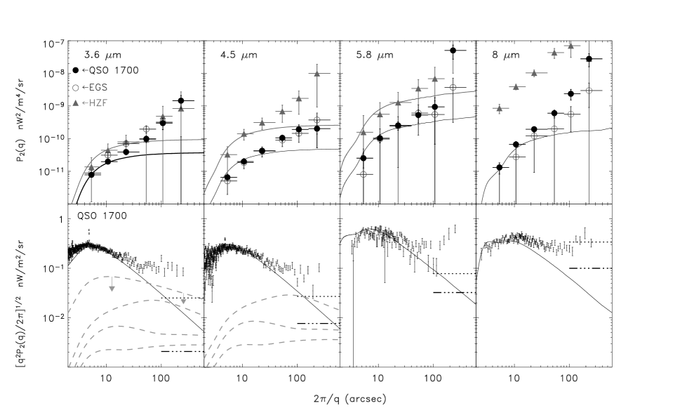
Figure 1: Spectrum of CIB fluctuations Top: Power spectrum of signal minus noise from the SI Fig. 2 averaged over wide bins to increase signal-to-noise. The errors are $N_{q}^{-1/2}$ corresponding to the cosmic variance, where $N_{q}$ is number of Fourier elements at the given $q$-bin. Solid lines show the shot noise from remaining galaxies fainter than the limiting magnitude in Table 1. Filled circles and the darkest shade error bars correspond to the QSO1700 data, open circles and intermediate shade error bars to the EGS data and triangles with the lightest shade error bars and lines correspond to HZF data. Bottom panels: fluctuations, $[\frac{q^{2}P(q)}{2\pi}]^{1/2}$, vs $2\pi/q$ for the QSO1700 data. Dashed lines estimate the contribution from ordinary galaxy populations and $\Lambda$CDM density field with $\Delta t$=5Gyr: the top dashed line shows the upper limit which assumes that their (high-$z$) clustering pattern remained identical to that today at $z$=0 and the other dashed lines correspond to $\langle z\rangle$=1,3,5 from top to bottom. Solid lines show shot noise from remaining ordinary galaxies. Dotted and dash-dot-dotted lines show the estimated Galactic cirrus and zodiacal light contributions respectively assuming the power spectra to be $P(q)\propto q^{n}$ with $n=-2$ typical of cloud distributions. The observed cirrus power spectrum is a little steeper with $n\sim-2.5$ to $-3$ [17, 49, 21, 50] in which case the lines will have a slope of $(3+n)/2$=0.25 to 0.5.

Figure 2: Colour properties of clipped maps Estimates of colour between channels 1 and 2. Circles correspond to $\sqrt{P_{2}/P_{1}}$, averaged over the bins centered at these angles, diamonds to $\langle\delta_{2}(x)\delta_{1}(x+\theta)\rangle/\langle\delta_{1}(x)\delta_{1}(x+\theta)\rangle$ for $N_{\rm cut}=4$ and triangles to the same quantity averaged over maps with $N_{\rm cut}=4,3,2.5,2$. Squares correspond to $\beta_{41}/\beta_{42}$ averaged over maps with $N_{\rm cut}=4,3,2.5,2$.

Figure 3: Contribution to CIB flux from Spitzer IRAC galaxy counts at 3.6 $\mu$m and 4.5 $\mu$m. The value of $dF/dm$ is evaluated from counts data and is a rapidly decreasing function of $m$ of the form $dF/dM\propto\exp(-bm)$ with $b\simeq 0.4$ (the least squares fits are shown with solid lines). (At the other two IRAC channels the uncertainty in the fall-off is much greater, but we show below that definite conclusions can already be reached from the data at 3.6 and 4.5 $\mu$m). Assuming that the functional form of $dF/dm$ does not begin to rise appreciably at still fainter magnitudes gives the CIB contribution from galaxies fainter than $m_{0}$ of $F(m>m_{0})=b^{-1}dF/dm|_{m_{0}}$. For the QSO 1700 field, we eliminate galaxies brighter than $m_{\rm Vega}\simeq 22.5$ at 3.6 $\mu$m and $m_{\rm Vega}\simeq 20.5$ at 4.5 $\mu$m corresponding to AB magnitudes $\simeq 25$ and $24$ respectively. The annotation in each panel show numbers which correspond to the extrapolated total flux from galaxies fainter than the magnitude limits in Table 1 using the least-squares fits shown with solid lines. One can expect that galactic spectra at the appropriate range of wavelengths are at most as steep as that of Vega, a star with a Rayleigh-Jeans black body spectral fall-off at these wavelengths. If so, they would generally have $K-m_{3.6}>0$ leaving galaxies with $K{{}_{>}\atop{}^{\sim}}22$ (e.g. [41]). Galaxies at K$>20$ have median redshift ${{}_{>}\atop{}^{\sim}}1$ ([42]), so the above argument would place the galaxies remaining at 4.5 $\mu$m at $z{{}_{>}\atop{}^{\sim}}1$ and those remaining at 3.6 $\mu$m still farther out to higher $z$. Comparison with the Lyman Break Galaxy candidates in the same area shows that a substantial fraction of these galaxies are at $z\sim 2-4$ with $z\sim 3$ being the median redshift [14]. Similarly, a substantial part of these galaxies are confirmed to be star-forming systems at $z\simeq 2.3$ ([43]).

Supplementary Information for “Tracing the first stars with cosmic infrared background fluctuations”

by A. Kashlinsky, R. G. Arendt, J. Mather, S. H. Moseley

This material presents technical details to support the discussion in the main paper. We discuss here data assembly, removal of individual resolved sources, computations of the power spectra and correlation functions from the maps cleaned off these sources, and evaluation of the Limber equation in the form used in the main paper. We also show maps of the cleaned field and present the plots with their power spectrum and that of the instrument noise.

Data processing

For this analysis the raw data were reduced using a least-squares self-calibration method (ref. [18] in main paper). This procedure models the raw data ($D^{i}$) of each frame as

$$D^{i}=G^{p}S^{\alpha}+F^{p}+F^{q}$$ (1)

where the index $i$ counts over all pixels of all frames, $S^{\alpha}$ is the sky intensity at location $\alpha$, $G^{p}$ is the detector gain at pixel $p$, $F^{p}$ is the detector offset at pixel $p$, and $F^{q}$ is an offset that can differ for each frame and each of the four detector readouts (combined into the index $q$). This self-calibration procedure has advantages over the standard pipeline calibration of the data in that the derived detector gain and offsets match the detector at the time of the observation, rather than at the time of the calibration observations. The most noticeable difference (especially at 3.6 and 8 ${\mu{\rm m}}$) is that the different AORs are affected by different patterns of residual images left by prior observations, which if not properly removed, can leave artifacts in the final images.

The combined use of low (QSO 1700) and high brightness (HZF) fields removes the gain-offset degeneracy in the self-calibration, although since we are interested in the nearly flat uniform background, to first order it is more important that the observing strategy included dithering to distinguish between detector and sky variations. Because IRAC’s calibration does not include zero-flux closed-shutter data, a degeneracy remains in the absolute zero point of the solution. The sky intensity $S^{\alpha}$ can be increased by a constant value at all locations $\alpha$, and the offset $F^{p}$ can be appropriately decreased without affecting the quality of the fit. A degeneracy also remains in first-order gradients (or two-dimensional linear backgrounds). The parameter $F^{q}$ can correlate with the dither position to induce false linear gradients in the other parameters without affecting the quality of the fit. However higher-order gradients are not degenerate. Because of these degeneracies, linear gradients have been fit and subtracted from the self-calibrated mosaicked images. Hence our estimates of the power at scales ${{}_{>}\atop{}^{\sim}}5^{\prime}$ should be treated as lower limits.

After the self-calibrations had been determined, corrections for “column pull-down” at 3.6 and 4.5 ${\mu{\rm m}}$ and banding or “row pull-up” at 8 ${\mu{\rm m}}$ were applied to the calibrated individual frames before mosaicking into a final image. Both these electronic effects only occur at bright sources, and are strictly aligned with the array coordinates and thus would also be minimized by selective filtering in the Fourier domain (discussed below). The column pull-down algorithm applied is the “do_pulldown” procedure which is available on the Spitzer Science Center (SSC) website as a contributed software tool for post-BCD (Basic Calibrated Data) processing. The row pull-up correction used at 8 ${\mu{\rm m}}$ adjusts each row of each frame as a function of the total flux above the 90th-percentile level of that row. The mosaicking built into the self-calibration is an interlacing algorithm, in which each datum ($D^{i}$) is averaged into only a single sky pixel ($S^{\alpha}$). This means that the random noise in $D^{i}$ translates into a completely random noise component in $S^{\alpha}$, but it also means that for sky maps with half-size pixels ($0.6{{}^{\prime\prime}}$) as we use here for the QSO 1700 data, the effective coverage for a sky pixel ($\alpha$) is reduced by a factor of 4.

Modeling Resolved Sources

In the full data set mosaics, the foreground sources were identified and measured using SExtractor (ref. [22] in main paper). The resulting source catalog is statistically consistent (within the Poissonian uncertainties) with the IRAC source counts (ref. [15] in main paper), both in terms of numbers of sources and limiting magnitudes. A model image of the foreground sky was then constructed by scaling an IRAC point spread function (PSF) image by the intensity of each source and adding it to an initially blank map at the appropriate location of each source. For one version of this, we used the PSFs that were determined during IOC and are available as FITS images on the SSC website. However, these PSFs are only mapped within a $\sim\ 24{{}^{\prime\prime}}\times 24{{}^{\prime\prime}}$ region, and thus neglect the extended low-level wings of the PSFs. Thus a second model was created in which the PSFs applied consisted of the IOC PSF cores smoothly grafted onto the extended wings as measured by observations of a bright (saturated) star. This wide grafted PSF avoids saturation at the core while tracing the extent out to the full size of the array ($\sim\ 300{{}^{\prime\prime}}\times 300{{}^{\prime\prime}}$). However, even with these wide PSFs, these models cannot account for the extended emission around many of the galaxies that are resolved by IRAC. Therefore we developed a final model, similar to a CLEAN algorithm (ref. [16] in main paper). To construct this model for each channel (1) the maximum pixel intensity was located (and saved to a list of “clean components”), (2) the wide PSF was scaled to half of this intensity and subtracted from the image, (3) this process was iterated 60,000 times, saving intermediate results every 3,000 iterations. The results were examined to identify the appropriate iteration number where the clean components become largely uncorrelated with the sources in the original image (i.e. they represent randomly distributed peaks without apparent convolution by the PSF). This limit occurs much more quickly in the longer wavelength channels, where the relative noise level is higher and the number of detected sources is fewer. The “model” is then the designated number of clean components convolved with the wide PSF. Since this model can represent extended emission with groups of clustered components, it is much better at removing the extended emission of the resolved galaxies. However, even this model will miss extended emission that is below the pixel-to-pixel noise. Such low surface brightness features must be dealt with as part of the analysis and interpretation of the power spectra.

Clipping individual sources

The original maps were clipped of resolved sources (Galactic stars and galaxies) using an iterative method developed for DIRBE data analysis (ref. [21] in main paper). Each iteration calculates the standard deviation ($\sigma$) of the image, and then masks all pixels exceeding $N_{\rm cut}\ \sigma$ along with $N_{\rm mask}\times N_{\rm mask}$ surrounding pixels. The procedure is repeated until no pixels exceed $N_{\rm cut}\ \sigma$. This clipping tends to miss emission in the outer parts of extended sources and the distant wings of very bright point sources. To help minimize this effect, the clipping (and subsequent analysis) is followed by subtraction of the models described above. We also clip the model images themselves with the same algorithm at the same level of $N_{\rm cut}$ with the mask derived from the clipping of the actual data field. The final mask was taken to be the combined mask from the two clipped maps, the main data and the model map. Whereas the appearance of the residual emission around bright sources has decreased dramatically with this extra step, the results were practically unaffected by this extra clipping (${{}_{<}\atop{}^{\sim}}$ a few percent in large scale power).

Truly robust results must be independent of the clipping parameters to within the variations from the signal arising from the populations of sources corresponding to the different clipping thresholds, $N_{\rm cut}$. We explored the range for the various clipping parameters: the results are largely independent of the mask size and in what follows a value of $N_{\rm mask}=3$ was adopted for displaying the final power spectra, which corresponds to ${{}_{>}\atop{}^{\sim}}75$ % pixels remaining in the clipped field at $N_{\rm cut}=4$. For sufficiently low values of $N_{\rm cut}$ too few pixels remained in the field for robust Fourier analysis of the diffuse light distribution. In order to further verify robustness of the results we also evaluated the correlation function at lower values of $N_{\rm cut}$ when significantly fewer pixels remained. This simple clipping algorithm proved quite efficient in identifying the sources. Comparison with the SExtractor model catalog shows that in channels 1 and 2 our clipping algorithm identified over 95% of the sources and in channel 3 and 4 the overlap with the SExtractor catalog was nearly 100%.

Computing power spectrum from clipped maps

The blanked pixels were assigned $\delta F$=0, thereby not adding power to the eventual power spectrum. Prior to computation of the Fourier transform and the correlation function, we subtracted remaining linear gradients from the maps. The Fourier transform image was cleansed of stripes and muxbleed artifacts in the $(u,v)$ transform space by zeroing the power at frequencies corresponding to $u=\pm nq_{mux}(n$= 1,2, 3,…) where $\pi/q_{mux}=4\times 1.2{{}^{\prime\prime}}$ which is the spacing of muxbleed artifacts. Power was also set to zero along the $u$=0 and $v$=0 axes to eliminate any residual signal from the gradient subtraction. The final power spectrum of the residual diffuse light was computed by averaging over narrow concentric rings of radius $q$. The noise was evaluated from the $A-B$ difference maps using the same clipping mask and weighting method as the final co-added data.

Fig. SI-1 shows the clipped maps for the QSO 1700 field used in the analysis and Fig. SI-3 plots the power spectra deduced from the clipped maps and their noise.

Figure SI-1: Point source subtracted and clipped ($N_{\rm cut}=4,N_{\rm mask}=3$) weighted intensity images of the QSO 1700 field for channels 1 through 4 (top to bottom). These positive images are aligned in the horizontal direction. They are scaled from [-2.0,4.0], [-2.2,4.4], [-9.2,18.4], and [-6.0,12] nW m^-2 sr^-1 respectively. These ranges are proportional to the standard deviation for each image. The regions of clipped sources are indicated by black areas which are set to 0.0 for further analysis.

Fig. SI-2 shows the maps clipped at $N_{\rm cut}=2$ with $N_{\rm mask}=3$. Lowering $N_{\rm cut}$ leaves huge multi-connected holes in the image. This precludes robustly computing Fourier transform of the maps; hence we evaluated the autocorrelation function, $C(\theta)=\langle\delta F(x+\theta)\delta F(x)\rangle$ for low $N_{\rm cut}$, which is shown in Fig. SI-4. The figure shows that at every level of $N_{\rm cut}$ we find the same large scale correlations with $C(\theta)$ remaining positive to at least $\simeq 100^{\prime\prime}$. (The slight drop in the amplitude with lower $N_{\rm cut}$ is expected as progressively lower peaks of CIB and the instrument noise are clipped). Note that the power spectrum, if of cosmological origin, may depend on $N_{\rm cut}$ if the clipping pushes deep enough to start eliminating the high-$z$ cosmological sources.

Figure SI-2: Same as Fig. SI-1, but for $N_{\rm cut}=2$.

Figure SI-3: Figure resolution reduced to conform to astro-ph reuqirements. Original figure available from http://haiti.gsfc.nasa.gov/kashlinsky/LIBRA/NATURE/. Signal and noise from QSO 1700 field (top), the HZF (bottom - red lines) and the EGS fields (bottom - blue lines). The power spectrum of the residual diffuse emissions (+noise) is plotted with its errors and the noise is shown with open diamonds. The errors correspond to $\sqrt{N_{q}}$, where $N_{q}$ is the number of Fourier elements that went into evaluating each value of $P_{2}(q)$.

Figure SI-4: Autocorrelation function for the QSO 1700 field for $N_{\rm cut}=2.5,3,4$. Thick lines correspond to $N_{\rm mask}=3$; thin lines to $N_{\rm mask}=5$. The fraction of clipped pixels in the QSO 1700 data at $N_{\rm cut}=4$ and $N_{\rm mask}=3$ is between 25% (4.5 $\mu$m) and 17 % (5.8 $\mu$m). Dotted lines show $\sqrt{|C(\theta)|}$ on scales where $C(\theta)<0$.

Systematic instrument effects

Systematic errors associated with the detector self-calibration, i.e. the gain (or flat field) and the offset (or dark frame), should produce a pattern on the sky which is the fixed pattern of the error convolved with the dither pattern of the pointings for each AOR. Since we do not know the pattern of the systematic error, we created mosaics from the detector flat fields, from the detector dark frames, and from frames consisting of a single Gaussian point source at a fixed position on the detector. Visually, the sort of structure that appears in these systematic error images does not look like the actual sky images. This is confirmed quantitatively by performing the power spectrum analysis on these images, which in all cases show fluctuations with a distinctly different spectrum from those of the real data. A different test for possible instrumental effects is to check the isotropy of the fluctuations. Instrumental effects (such as muxbleed, column pull-down, etc.) are likely to be associated with preferred directions on the array and on the sky as well since the position angle of the detector was roughly constant for the duration of the observations. As a test of isotropy for each channel we calculated the power spectra in four 45^∘-wide azimuthal sectors of the Fourier transform’s $(u,v)$ plane centered along the lines $v=0$, $v=u$, $u=0$, and $v=-u$. The sectors along the axes would be expected to be more strongly affected by instrumental effects, but we find that there are no large-scale variations between the power spectra in the different sectors and only ${{}_{<}\atop{}^{\sim}}5\%$ variations in the overall amplitudes. Stray light is a systematic error which remains relatively fixed with respect to the sky rather than with respect to the detector. There is only one star (SAO 17323, $m_{V}=8.8$, $m_{K}=7.6$) in the region of the QSO 1700 field which produces visible stray light artifacts in Channels 1 and 2 (stray light paths are different for channels 3 and 4). However, the structure of these artifacts are different in Channels 1 and 2, and more important they appear in the lower coverage edges of the full images which are excluded from the power spectrum analysis.

Interpretation of the signal with Limber equation

More details related to this section can be found in ref. [2] of the main paper. Whenever CIB studies encompass relatively small parts of the sky (angular scales $\theta<1$ radian) one can use Cartesian formulation of the Fourier analysis. If the fluctuation field, $\delta F(\mbox{\boldmath$x$})$, is a random variable, then it can be described by the moments of its probability distribution function. The first non-trivial moment is the projected 2-dimensional correlation function $C(\theta)=\langle\delta F(\mbox{\boldmath$x$}+\theta)\delta F(\mbox{\boldmath$x$})\rangle$. The 2-dimensional power spectrum is $P_{2}(q)\equiv\langle|\delta F_{q}|^{2}\rangle$, where the average is performed over all phases. The correlation function and the power spectrum are a pair of 2-dimensional integral transforms, $P_{2}(q)=2\pi\int_{0}^{\infty}C(\theta)J_{0}(q\theta)\theta d\theta$. In the limit of small angles, the projected 2-dimensional correlation function is related to the CIB flux production rate, $dF/dz$, and the evolving 3-D power spectrum of galaxy clustering, $P_{3}(k)$, via the Limber equation given by:

$$C(\theta)=\int dz{\left(\frac{dF}{dz}\right)}^{2}\int_{-\infty}^{\infty}\xi(r;z)du$$ (2)

where $r^{2}=c^{2}(dt/dz)^{2}u^{2}+d_{A}^{2}\theta^{2}$ and $\xi(r)=\frac{1}{2\pi^{2}}\int P_{3}(k)j_{0}(kr)k^{2}dk$ is the two point correlation function for 3-dimensional clustering with the power spectrum $P_{3}(k)$. In the power spectrum formulation this equation can be written as (see e.g. refs. [2,12,13,21] of the main paper for details):

$$P_{2}(q)=\int\left(\frac{dF}{dz}\right)^{2}\frac{1}{c\frac{dt}{dz}d_{A}^{2}(z)}P_{3}(qd_{A}^{-1};z)dz=\frac{1}{c}\int\left(\frac{dF}{dt}\right)^{2}\frac{1}{d_{A}^{2}(z)}dt$$ (3)

where $d_{A}(z)$ is the comoving angular diameter distance and the integration is over the epoch of the sources contributing to the CIB. Multiplying both sides of this equation by $q^{2}/2\pi$ leads, after simple algebra, to eqs. (1),(2) in the main text of the paper. The fluctuation of the CIB on angular scale $2\pi/q$ can then be expressed as:

$$\sqrt{\frac{q^{2}P_{2}(q)}{2\pi}}=F_{\rm CIB}\Delta(qd_{A}^{-1}(\langle z\rangle))$$ (4)

where the suitably averaged redshift $\langle z\rangle$ is given by:

$$\Delta^{2}(qd_{A}^{-1}(\langle z\rangle))\equiv\frac{\int dt\int(dF/dt)^{2}\Delta^{2}(qd_{A}^{-1}(z))dt}{[\int(dF/dt)dt]^{2}}$$ (5)

In other words, the fractional fluctuation on angular scale $\pi/q$ in the CIB is given by the average value of the r.m.s. fluctuation from spatial clustering over a cylinder of length $ct_{0}$ and diameter $\sim q^{-1}d_{A}^{-1}(\langle z\rangle)$ at the effective redshift given above.

References and Notes

- [1] Hauser, M. G. & Dwek, E. The Cosmic Infrared Background: Measurements and Implications, Ann.Rev.Astron.Astrophys., 39,249-307 (2001)
- [2] Kashlinsky, A. Cosmic infrared background and early galaxy evolution, Phys. Rep., 409, 361-438 . (2005)
- [3] Kogut, A. et al. First Year Wilkinson Microwave Anisotropy Probe (WMAP) Observations: Temperature-Polarization Correlation, Astrophys.J.Suppl., 148, 161-173 (2003)
- [4] Bennett, C. et al. First-Year Wilkinson Microwave Anisotropy Probe (WMAP) Observations: Preliminary Maps and Basic Results, Astrophys.J.Suppl., 148,1-37
- [5] Abel, T. et al. The Formation of the First Star in the Universe, Science, 295, 93-98 (2002)
- [6] Bromm, V. et al. Forming the First Stars in the Universe: The Fragmentation of Primordial Gas, Astrophys.J., 527, L5-L8 (1999)
- [7] Rees, M.J. Origin of pregalactic microwave background, Nature, 275, 35-37 (1978)
- [8] Kashlinsky, A., Mather, J. & Odenwald, S. Clustering of the diffuse infrared light from the COBE DIRBE maps. IV. Overall results and possible interpretations, preprint (1999)
- [9] Salvaterra, R. & Ferrara, A. The imprint of the cosmic dark ages on the near-infrared background, Mon.Not.R.Astr.Soc., 339, 973-982 (2003)
- [10] Magliochetti, M., Salvaterra, R. & Ferrara, A. First stars contribution to the near-infrared background fluctuations, Mon.Not.R.Astr.Soc., 342, L25-L29 (2003)
- [11] Santos, M., Bromm, V. & Kamionkowski, M. The contribution of the first stars to the cosmic infrared background, Mon.Not.R.Astr.Soc., 336, 1082-1092 (2002)
- [12] Cooray, A., Bock, J., Keating, B., Lange, A. & Matsumoto, T. First Star Signature in Infrared Background Anisotropies, Astrophys.J.., 606, 611-624 (2004)
- [13] Kashlinsky, A., Arendt, R., Gardner, J.P., Mather, J., & Moseley, S.H. Detecting Population III Stars through Observations of Near-Infrared Cosmic Infrared Background Anisotropies, Astrophys.J.,608, 1-9 (2004)
- [14] Barmby, P. et al. Deep Mid-Infrared Observations of Lyman Break Galaxies, Astrophys.J.. Suppl., 154, 97-102 (2004)
- [15] Fazio, G. G. et al. Number Counts at 3 m 10 m from the Spitzer Space Telescope, Astrophys.J.. Suppl., 154, 39-43 (2004)
- [16] Hgbom, J. Aperture Synthesis with a Non-Regular Distribution of Interferometer Baselines, Astrophys.J.Suppl., 15,417-426 (1974)
- [17] Gautier, T. N., Boulanger, F. Perault, M., Puget, J. L. A calculation of confusion noise due to infrared cirrus, Astron. J., 103, 1313-1324. (1992)
- [18] Fixsen, D. J., Moseley, S. H. & Arendt, R. G. Calibrating Array Detectors, Astrophys.J.. Suppl., 128, 651-658 (2000)
- [19] Fazio, G. G. et al The Infrared Array Camera (IRAC) for the Spitzer Space Telescope, Astrophys.J.. Suppl., 154, 10-17 (2004)
- [20] Hauser, M. G. et al. The COBE Diffuse Infrared Background Experiment Search for the Cosmic Infrared Background. I. Limits and Detections, Astrophys.J., 508, 25-43 (1998)
- [21] Kashlinsky, A. & Odenwald, S. Clustering of the Diffuse Infrared Light from the COBE DIRBE Maps. III. Power Spectrum Analysis and Excess Isotropic Component of Fluctuations, Astrophys.J., 528, 74-95 (2000)
- [22] Bertin, E. & Arnouts, S. SExtractor: Software for source extraction., Astron.Astrophys. Suppl., 117, 393-404 (1996)
- [23] Wright, E.L. DIRBE minus 2MASS: Confirming the Cosmic Infrared Background at 2.2 Microns, Astrophys.J., 553, 538-544 (2001)
- [24] Arendt, R. et al. The COBE Diffuse Infrared Background Experiment Search for the Cosmic Infrared Background. III. Separation of Galactic Emission from the Infrared Sky Brightness, Astrophys.J., 508,74-105 (1998)
- [25] Efstathiou, G., Sutherland, W.J. & Maddox, S.J. The cosmological constant and cold dark matter, Nature, 348, 705-707 (1990)
- [26] Tegmark, M. et al. Cosmological parameters from SDSS and WMAP, Phys.Rev.D. 69, 103501-103527 (2004)
- [27] Kaiser, N. On the spatial correlations of Abell clusters, Astrophys.J., 284, L9-L12 (1984)
- [28] Dwek, E. & Arendt, R. A Tentative Detection of the Cosmic Infrared Background at 3.5 m from COBE/DIRBE Observations, Astrophys.J., 508, L9-L12 (1998)
- [29] Matsumoto, T. et al Infrared Telescope in Space Observations of the Near-Infrared Extragalactic Background Light, Astrophys.J., 626, 31-43 (2005)
- [30] Wright, E.L. & Reese, E.D. Detection of the Cosmic Infrared Background at 2.2 and 3.5 Microns Using DIRBE Observations, Astrophys.J., 545,43-55 (2000)
- [31] Gorjian, V., Wright, E.L. & Chary, R.R. Tentative Detection of the Cosmic Infrared Background at 2.2 and 3.5 Microns Using Ground-based and Space-based Observations, Astrophys.J., 536, 550-560 (2000)
- [32] Cambresy, L., Reach, W. T., Beichman, C.A. & Jarrett, T. H. The Cosmic Infrared Background at 1.25 and 2.2 Microns Using DIRBE and 2MASS: A Contribution Not Due to Galaxies?, Astrophys.J., 555, 563-571 (2001)
- [33] Kashlinsky, A., Odenwald, S., Mather, J., Skrutskie, M. & Cutri, R. Detection of Small-Scale Fluctuations in the Near-Infrared Cosmic Infrared Background from Long-Exposure 2MASS Fields, Astrophys.J., 579, L53-L57 (2002)
- [34] Odenwald, S., Kashlinsky, A., Mather, J., Skrutskie, M. & Cutri, R. Analysis of the Diffuse Near-Infrared Emission from Two-Micron All-Sky Survey Deep Integration Data: Foregrounds versus the Cosmic Infrared Background, Astrophys.J., 583, 535-550 (2003)
- [35] Springel, V. et al. Siumulations of the formation, evolution and clustering of galaxies and quasars, Nature, 435, 629-636 (2005)
- [36] Kelsall, T., et al. The COBE Diffuse Infrared Background Experiment Search for the Cosmic Infrared Background. II. Model of the Interplanetary Dust Cloud, Astrophys.J., 508, 44-73 (1998)
- [37] Bromm, V. & Larson, R.B. The First Stars, Ann.Rev.Astron.Astrophys., 42, 79-118 (2004)
- [38] Miralda-Escude, J. The Dark Age of the Universe, Science, 300, 1904-1909 (2003)
- [39] Kashlinsky, A. Reconstructing the Spectrum of the Pregalactic Density Field from Astronomical Data, Astrophys.J., 492, 1-28 (1998)
- [40] Schlegel, E. M., Finkbeiner, D. P., & Davis, M. Maps of Dust Infrared Emission for Use in Estimation of Reddening and Cosmic Microwave Background Radiation Foregrounds, Astrophys.J., 500, 525-553 (1998)
- [41] Eisenhardt, P.R. et al. The Infrared Array Camera (IRAC) Shallow Survey, Astrophys.J.Suppl, 154, 48-53 (2004)
- [42] Cowie, L.L. et al New Insight on Galaxy Formation and Evolution From Keck Spectroscopy of the Hawaii Deep Fields, Astron.J., 112, 839-864 (1996)
- [43] Shapley, A.E. et al Ultraviolet to Mid-Infrared Observations of Star-forming Galaxies at z2: Stellar Masses and Stellar Populations, Astrophys.J., 626, 698-722 (2005)
- [44] Peacock, J. and Dodds, S.J. Non-linear evolution of cosmological power spectra, 1996, Mon.Not.R.Astr.Soc., 280, L19-L26 (1996)
- [45] Steidel, C. et al. Spectroscopic Identification of a Protocluster at z=2.300: Environmental Dependence of Galaxy Properties at High Redshift, Astrophys.J., 626, 44-50 (2005)
- [46] Maddox, S., Efstathiou, G., Sutherland, W., Loveday, J. Galaxy correlations on large scales, Mon.Not.R.Astr.Soc., 242, 43P-47P (1990)
- [47] Perlmutter, S. et al. Measurements of Omega and Lambda from 42 High-Redshift Supernovae, Astrophys.J., 517, 565-586 (1999)
- [48] Oliver, S. et al. Angular Clustering of Galaxies at 3.6 Microns from the Spitzer Wide-area Infrared Extragalactic (SWIRE) Survey, Astrophys. J. Suppl., 154, 30-34 (2004)
- [49] Ingalls, J.G. et al. Structure and Colors of Diffuse Emission in the Spitzer Galactic First Look Survey, Astrophys. J., 154, 281-285 (2004)
- [50] Wright, E.L. Angular Power Spectra of the COBE DIRBE Maps, Astrophys. J., 496, 1-8 (1998)