An unbiased search for the signatures of protostars in the $\rho$ Ophiuchi Molecular Cloud

The dense cores which conceive and cradle young stars can be explored through continuum emission from associated dust grains. We have performed a wide field survey for dust sources at 1.2 millimetres in the $\rho$ Ophiuchi molecular cloud, covering more than 1 square degree in an unbiased fashion. We detect a number of previously unknown sources, ranging from extended cores over compact, starless cores to envelopes surrounding young stellar objects of Class 0, Class I, and Class II type. We analyse the mass distribution, spatial distribution and the potential equilibrium of the cores. For the inner regions, the survey results are consistent with the findings of previous narrower surveys. The core mass function resembles the stellar initial mass function, with the core mass function shifted by a factor of two to higher masses (for the chosen opacity and temperature). In addition, we find no statistical variation in the core mass function between the crowded inner regions and those in more isolated fields except for the absence of the most massive cores in the extended cloud. The inner region contains compacter cores. This is interpreted as due to a medium of higher mean pressure although strong pressure variations are evident in each region. The cores display a hierarchical spatial distribution with no preferred separation scale length. However, the frequency distribution of nearest neighbours displays two peaks, one of which at 5000 AU can be the result of core fragmentation. The orientations of the major axes of cores are consistent with an isotropic distribution. In contrast, the relative orientations of core pairs are preferentially in the NW-SE direction on all separation scales. These results are consistent with core production and evolution in a turbulent environment. Finally, we report the discovery of a new, low-mass Class 0 object candidate and its CO outflow.

1 Introduction

As one of the nearest star-forming regions, the $\rho$ Ophiuchi molecular cloud complex has been the target of numerous investigations. A prime focus has been the densest part of the L 1688 cloud which harbours a large number of young stellar objects, studied at near- to mid-infrared wavelengths (Vrba et al. 1975; Elias 1978; Wilking et al. 1989; Barsony et al. 1989; Comeron et al. 1993; Luhman & Rieke 1999; Wilking et al. 2001; Bontemps et al. 2001; Allen et al. 2002) and at (sub)millimetre wavelengths (Andre et al. 1993; Andre & Montmerle 1994; Nürnberger et al. 1998; Wilson et al. 1999; Tachihara et al. 2000). To investigate how these stars are conceived, we wish to to relate their properties to those of the embedding cloud of molecular gas and dust which both nurture and obscure the stars. However, technical capabilities restrict the field over which area-covering surveys can be undertaken, bearing the danger of picking peculiar objects prevalent in the “more interesting” parts, thus biasing the results obtained from statistical investigations. In order to further exclude such selection effects, we have performed an unbiased survey of a wide area around the L 1688 molecular cloud for dust continuum sources, including the dense molecular cores as well as the areas which apparently do not harbour dense molecular material.

The entire star formation complex extends over several degrees on the sky (Loren 1989a), containing a few major clouds. The L 1688 cloud is situated about one degree south of the $ρ$~Ophiuchus star itself. This ‘main cloud’ of $\rho$ Oph covers an area of roughly 480 arcmin² and has been dissected into about a dozen cloud components (Mezger et al. 1992). This area was surveyed at 1.3 mm by Motte et al. (1998, hereafter MAN98), who uncovered 62 starless cores and 41 circumstellar structures. These observations had a resolution of just 11 arcsec, corresponding to 1,400 AU. The inferred distribution of masses of these cores was found to be comparable to the stellar initial mass function, suggesting that stellar masses are determined at conception. Subsequently, the results of a larger, somewhat more sensitive survey at 0.85 mm were presented by Johnstone et al. (2000) (hereafter J00). This survey covered $\sim$ 700 arcmin² with a resolution of 14 arcsec, identifying 55 cores. This survey was recently followed up by a much more extensive (4 square degrees) but significantly more shallow survey by Johnstone et al. (2004) (hereafter J04), mainly extending to the north/north-west of the main cloud.

In the present 1.2 mm survey, we cover an area of 4,600 arcmin². This constitutes a significant extension to the above works although the resolution is $\sim$24″. Our immediate goals are to (i) derive the core masses (§3), (ii) estimate the mass relative to a critical Bonnor-Ebert sphere or Jeans mass by including the core sizes (§4), (iii) quantify the spatial distribution and orientations (§5 & §B), and (iv) quantify the mass distribution (§6). In addition, we report the discovery of a new low-mass candidate Class 0 source and its CO outflow (§7). A companion paper (Khanzadyan et al. 2004) presents the results of a near-infrared imaging search for protostellar H₂ outflows over a large section of the present survey area. Finally, the core, outflow and protostellar properties will be related in detail in a forthcoming paper.

Quoted distances to the $\rho$ Ophiuchi cloud lie in the range $D=$ 125 – 165 pc, as recently summarised by Rebull et al. (2004). de Geus et al. (1989) analysed photometry of the stars in the nearby Sco OB2 association. It was shown that the Ophiuchus dark clouds are on the near side of Upper Scorpius, at $\sim$ 125 pc. Hipparcos data confirm the distance to Upper Scorpius and yield a distance of $\sim$ 128 pc to the quadruple $\rho$ Oph system (de Zeeuw et al. 1999). Here, we shall follow the suggestion by Rebull et al. (2004) and take the weighted average distance of 130 pc.

In the following, we will designate all well-defined low mass structures as ‘cores’ (with mass below about $50\,$M_⊙) and apply the term ‘clump’ to more massive structures defined through low resolution CO mapping. A clump usually corresponds spatially to a cluster of cores.

2 Observations

available as jpg: 0511093.1331f01.jpg
full postscript version available at http://www.ifa.hawaii.edu//users/stanke/preprints.html

Figure 1: SIMBA 1.2 mm continuum mosaic image of the $\rho$–Ophiuchi cloud. Intensity scaling is in mJy/beam (linear). Prominent clumps are marked as A, B1/1, C, D, E, and F. Dashed lines mark some filamentary structures east of the major clumps, with three more compact sources (MMS038, MMS051, and MMS126) within them also labeled. MMS126 is identified as a new, low-mass Class 0 object candidate in Sect. 7.

The observations were carried out using the SIMBA bolometer array at the SEST telescope on La Silla/Chile during an observing run lasting from 2002 July 7 to 12. SIMBA is a 37-channel bolometer array, operating at 1.2 mm, and provides a HPBW of $\sim$24″ (as measured on maps of Uranus). The weather was good and fairly stable with zenith opacities ranging between 0.17 and $\sim$ 0.3. In total, 78 maps in the fast mapping mode were taken (i.e., no wobbler was used). Typical map sizes were 1200″$\times$800″ with a scanning velocity of 80″/sec and 8″ steps between subscans. A number of maps were taken with a scanning velocity of 160″/sec (size 1800″$\times$800″) in order to improve sensitivity for extended structures. Pointing and focus were checked regularly; pointing corrections were typically a few arcsec and always below 10″. Skydips were taken every 1 to 2 hours, and Uranus was mapped several times for calibration purposes.

The data reduction was performed with MOPSI, a software package developed by Robert Zylka, following standard bolometer data reduction principles. First, noisy or dead channels were identified and deleted. Then, a low order baseline was subtracted from the data and an initial de-spiking was made. The data direct from the telescope consist of the true signal convolved with the response of the electronics, hence requiring deconvolution (Reichertz et al. 2001; Weferling et al. 2002). We chose to reconstruct the signal at a specific time using only data from a given window (typically 6 seconds) around this time, including the data recorded during the “turning” of the telescope between two on-map sub-scans (in the standard deconvolution only data taken during the on-map subscans are used, and the signal is reconstructed from the entire on-map sub-scan). This deconvolution was found to provide significantly better results than the standard deconvolution, for two reasons: the restriction to a shorter time span reduces noise that goes into the reconstruction of a given data point, and including the time during the turning of the telescope ensures a proper reconstruction of the data at the edges of the map, as sky fluctuations during turning (which are convolved into the data recorded during the on-map subscans) are properly taken out of the data recorded during the on-map subscans. Then, after the deconvolution, the data corresponding to off-map data taken during the turning of the telescope were deleted. After further low-order baseline corrections, correction for atmospheric extinction and correction for gain-elevation effects, correlated sky brightness variations (sky-noise) were removed. Here, an iterative procedure was used: for each iteration, we used the resulting mosaic of the previous iteration as an input model for the brightness distribution. Following another careful de-spiking and baseline subtraction, the data were then combined into a mosaic, weighting individual maps according to their noise (1/rms²). After each iteration, for each sub-map the polygons defining emission-free regions to be used for baseline fitting were carefully checked and, if necessary, adjusted, followed by a check of the degree of the polynomial used for baseline subtraction.

The noise level in the final mosaic is of the order of 10 mJy/beam throughout most of the map. Close to the edges, it degrades to 12-15 mJy/beam. For a point source, assuming a flux-to-mass conversion as outlined below, this corresponds to a 3$\sigma$ detection limit of the order of 0.014 M_⊙. In terms of column density, the 1$\sigma$ noise level corresponds to about 1.3$\times 10^{21}$cm^-2. This is slightly better than the 1.3 mm survey done by MAN98, but somewhat less sensitive than the J00 850$\mu$m survey; it is significantly more sensitive than the recent J04 850$\mu$m survey.

Similar to other (sub)millimetre surveys, our new map is sensitive only to sufficiently small structures (see also J00 for a discussion of this issue). In the case of SIMBA fast mapping observations, this is due to two effects: the subtraction of the sky emission removes any flux due to large scale, more or less uniform emission, and a high-pass filter applied to the signal from the bolometer will further suppress large-scale emission features. On top of these technical effects, baseline subtraction may further contribute; however, baseline subtraction was done very carefully in order to minimise this. Filtering of low frequencies and residuals from the deconvolution of the data are responsible for residual negative map values close to the brightest parts of the mosaic (dipping to $\sim$-20 mJy/beam (-2 $\sigma$) in the most negative patches), a feature generally found in SIMBA maps.

3 Data Analysis

available as jpg: 0511093.1331f02.jpg
full postscript version available at http://www.ifa.hawaii.edu//users/stanke/preprints.html

Figure 2: Model of the 1.2 mm continuum emission derived from the superposition of models for the 143 sources identified from the SIMBA data. Intensity scaling is in mJy/beam (linear).

available as jpg: 0511093.1331f03.jpg
full postscript version available at http://www.ifa.hawaii.edu//users/stanke/preprints.html

Figure 3: Residual after subtracting the model source distribution (Fig. 2) from the 1.2 mm mosaic (Fig. 1). Intensity scaling is in mJy/beam (linear).

The final 1.2 mm mosaic is shown in Fig. 1. In line with previous (sub)millimetre maps, a large variety of sources is seen, ranging from extended cores over more compact features to unresolved point sources. In those regions which were also covered by the MAN98 and J00 surveys we generally see a very good agreement between the different data sets (limited by the poorer angular resolution of our new data).

In the part of the mosaic which had not been previously observed, besides a number of fainter, extended structures, two more remarkable features turned up. On the one hand, there is a filamentary structure (dashed lines in Fig. 1) to the east of the previously revealed cores Oph-B/C/E/F, containing two more compact sources (MMS126 and MMS038/MMS051). MMS126 appears to be a newly discovered, low-mass Class 0 source (see Sect. 7 for details).

The second remarkable structure is the presence of a bright dust core MMS041 at the tip of the cometary dark cloud L 1696B. A similar core was already found in the neighbouring cloud L 1696 by MAN98.

3.1 Source identification

The variety in source morphologies makes a detailed source identification mandatory: e.g., using simple source detection algorithms with a certain detection threshold will not identify extended structures, which are clearly present, but might have maximum surface brightnesses of the order of the 1$\sigma$ noise level. To account for this, sources were identified using a wavelet decomposition similar to the method used by MAN98.

The final map was split into 5 planes using the TRANSFORM/WAVE and EXTRACT/WAVE tasks provided by the ESO/MIDAS wavelet context package. We will refer to the most compact scale as scale 1, and scale 2, 3, 4, and 5 to the next more extended scales.

We then used the 2-D adaption of the clumpfind algorithm developed by Williams et al. (1994) to identify features in the 5 planes individually. The lower limits for source identifications were set to 3-4 times the rms fluctuation of emission-free parts of the respective planes, with contours spaced by about 1 rms. The minimum number of pixels required to identify a sufficiently bright feature as a source was set according to the characteristic scale of each plane (i.e., to very small for scale 1, and getting bigger for larger scales). The thus detected features were then visually inspected to reject false detections due to residual scanning artifacts (found to be restricted to scales 1 and 2) or other misidentifications.

From the list of features identified at the various scales a final source list was compiled, including all features identified in scale 1, and all sources in the more extended scales which did not overlap with sources identified in the next more compact scale (i.e., for each feature we determined the part of the clump area as given by the clumpfind routine, in which the intensity was greater than 1/2 the maximum intensity, and checked if it overlapped with the corresponding area of all features of the next more compact scale). This resulted in a list of 139 sources (MMS001 to MMS139).

To this list we added 4 sources, MMS140 to MMS143, after visual inspection: while MMS141 is just too faint to be detectable in the individual planes, MMS140, MMS142, and MMS143 are small cores adjacent to large bright features, which make them hard to detect as taking out the extended scales creates negative haloes around large bright cores.

A full finding chart showing the location of all 143 sources is shown in Fig. 14 (online version only), and closeups of crowded regions are shown in Figs. 15, 16, and 17 (online version only).

Table 2 (online version only) lists the 1.2 mm sources found in our survey in the order they were identified by the wavelet decomposition plus clumpfind technique. In addition to the source position, it holds the integrated source flux and the peak flux determined in various ways, the major and minor axis and the position angle of the major axis, cross-identifications to the sources identified by Motte et al. (1998) and Johnstone et al. (2000), and a comment on association with known YSOs. In Section A we give notes on the individual sources.

3.2 Measuring source properties

Figure 4: The locations of all the 143 cores detected here (squares) compared to all the cores detected by J00 (asterisks). The coordinates are centred on -16:26:58.4, -24:45:36 (2000). A, B, and E mark the location of prominent clumps.

Figure 5: The locations of the 111 starless cores detected here (squares) compared to the the starless cores detected by MAN98 (asterisks). The circle is that employed to separate inner cores from the outer regions.

We then performed a detailed modelling of the overall brightness distribution using Gaussian sources, the result of which is shown in Fig. 2 (Fig. 3 shows the residual, after subtracting the model source distribution from the mosaic). In some cases, more than one Gaussian component centered on the source position had to be assumed in order to properly reproduce the shape of the sources (e.g., a bright source with a radial intensity distribution falling off as a power law will not be satisfactorily fitted by a single Gaussian).

The sources we detect within the inner core-crowded region are generally coincident with those found in previous surveys. Figs. 4 and 5 show that this is true for separate samples of all cores and starless cores. In particular, we recover all the cores from J00, despite the different observing wavelength. This confirms the reliability of our core-finding technique.

The fluxes of the sources were determined by first subtracting the model for all other sources from the mosaic, and then integrating over a certain area around the source within some given radius or (for more complex sources) within a certain polygon around the centre of the source. Similarly, sizes and position angles for each source were determined by (single) Gaussian fits to the mosaic with the model for all other sources subtracted.

Peak fluxes were calculated in four differing ways and are also given in Table 2: the column labelled as F_peak (a) gives the peak flux obtained from searching the maximum pixel value in an ellipse (with the minor and major axes as given in the table) around the peak position; F_peak (b) is the same as (a), but using only the sum of scales 5 down to the scale where the source was detected first; F_peak (c) gives the maximum pixel value in the same ellipse after re-binning according to the size of the sources minor axis (i.e., by FWHM_min/24″pixels); F_peak (d) gives the maximum pixel value of the model of the source. As done in deriving the total source flux, the models of all other sources were subtracted from the mosaic before determining the respective peak fluxes.

Depending on the source morphology and brightness, one or the other method can be expected to yield more accurate results. Relatively bright, compact sources should be best represented by F_peak (a), whereas faint, extended sources should be best measured by F_peak (b) or (c). Generally, the results agree well, apart from an obvious overestimate for large, low surface-brightness sources using the first method and systematic underestimates for compact sources using the second and third methods.

At this point it might be worth adding a note on the dependency of the effective mass/column density sensitivity limit on source size. The surveys of J00 and J04 identified sources setting a fixed threshold in peak flux, i.e., column density. In contrast, we also include sources whose surface brightness is nominally lower than, e.g., 3$\sigma$, but which are still clearly recognised because they are extended (the MAN98 analysis using a wavelet decomposition might be comparable in this respect). This introduces a size-dependent column density limit: for a source which has twice the radius ${\rm R}$, we can rebin the mosaic by 2$\times$2 pixels, effectively reducing the noise by a factor of two. I.e., the column density detection limit scales as ${\rm R}^{-1}$, which implies a mass detection limit scaling as ${\rm R}^{1}$ (whereas a fixed surface brightness cutoff implies a mass detection limit scaling as ${\rm R}^{2}$; always assuming that all sources have the same temperature and dust properties). In this sense, we can expect that our method of source identification yields, for a given mass, a more complete census than applying simply a column density cutoff, because it also includes the more extended, hence fainter (in surface brightness), sources.

Our method of source identification yielded significantly more sources than identified by J00 in areas covered by both surveys, despite the somewhat poorer angular resolution and slightly lower sensitivity. This is due to two reasons. First, J00 explicitly filter out more extended emission before applying clumpfind, thus removing extended features and lowering the signal also for more compact features. Second, they limit their identification to features with a given column density threshold, again biasing against low surface brightness, extended sources. Detailed comparison of our data with the J00 map before filtering out the extended emission shows that virtually all features that we identify are also seen on the J00 map, even if not identified in their list of objects. We have marked those features as ’n.i.’ in the ’J00’ column of Tab. 2.

4 Core Properties

4.1 Masses and column densities

Figure 6: Upper Panel: The mass and radius derived from the observations for each core. The crosses correspond to the 79 cores found within the central circle of radius 0.2^∘ shown in Fig. 12 and diamonds to those 64 outside. Lines of constant column density are overplotted for reference as dashed lines, with columns of atomic hydrogen from $3\times 10^{21}$ cm^-2 (right) to $3\times 10^{22}$ cm^-2 (left). The solid line marks the detection limit. Lower Panel: The masses and radii for just the starless cores, consisting of 62 within the circle (crosses) and 49 outside (diamonds).

Figure 7: The number distribution of the mean column density of the cores (also proportional to the surface pressure predicted if a sub-sample were critical Bonnor-Ebert spheres, as given from Eq. 3). Upper Panel: The full sample of 143 cores, with 79 within the inner crowded core and 64 external to it; lower Panel: the same distribution for just the starless cores (111 in total, 62 within the inner crowded core and 49 external to it).

The mass of each core is estimated on assuming it to be proportional to the measured 1.2 mm flux. The radiation is taken to be emitted from cool dust grains and the intervening medium is optically thin. The standard formulae for black bodies then yield the core masses from the fluxes $S_{1.2mm}$ expressed in Janskys (e.g MAN98 and J00):

$$M_{c}=0.58\times S_{1.2mm}\leavevmode\nobreak\ \leavevmode\nobreak\ \left[\frac{\kappa_{1.2mm}}{0.005\leavevmode\nobreak\ {\rm cm}^{2}\leavevmode\nobreak\ {\rm g}^{-1}}\right]^{-1}\cdot\\ \left[\exp\left(\frac{12\leavevmode\nobreak\ {\rm K}}{T_{d}}\right)-1\right]\left[\frac{D}{130\leavevmode\nobreak\ {\rm pc}}\right]^{2}{\rm M}_{\odot}.$$ (1)

Here, we take a fixed opacity at 1.2 mm of $\kappa$ = 0.005 cm² g^-1 and a fixed dust temperature of $T_{d}$ = 20 K. It should be noted that these quantities may vary across the cloud by a factor of order two, as fully discussed by MAN98 and J00.

The derived masses are plotted as a function of core size in Fig. 6. Here, we do not attempt to deconvolve the apparent cloud dimensions and define the mean observed clump angular radius of $\theta$ = 0.5 (FWHM_maj $\times$ FWHM_min)^1/2 from the FWHMs of the major and minor axes given in Table 2.

Although the inferred masses and radii are widely distributed, a mass-radius correlation is evident in Fig. 6. However, it should be remarked that large, low-surface brightness features might have been supressed by the observational procedure and data reduction, as discussed above. Hence, the apparent correlation is possibly only produced by a deficiency of extended, moderately massive features. (It should be noted that the smallest core radii presented in the diagram are at the limit of our resolution and subject to significant error). At small radii and masses, the lower envelope to the distribution of sources reasonably well reproduces the size dependency of the mass detection limit as argued above, ${\rm M}_{\rm lim}\propto{\rm R}$. To investigate a possible mass-radius correlation, locii of constant average column density, corresponding to $\log{\rm M}\propto 2\log{\rm R}_{c}$, are overplotted in Fig. 6. This demonstrates that at low radii and masses the detection limit yields a lower envelope to the distribution which influences the correlation.

Splitting the sample into cores within the inner, crowded region (marked by crosses, corresponding to the region investigated by MAN98 and J00) and those spread over the extended cloud (diamonds) hints at distinct lower envelopes for cores in the inner and outer regions, corresponding to average atomic hydrogen columns of $8\times 10^{21}$ cm^-2 (inner region) and $4\times 10^{21}$ cm^-2 (outer regions). We believe that this is at least partially due to observational limitations, as low surface-brighntess features are hard to identify in the crowded central region.

The number distribution for the core columns is displayed in Figure 7. This demonstrates that the offset in column density between the inner and outer regions is real and extends to the entire distribution and not just the lower bound to the column density. It is not caused only by a (possibly obervationally introduced) deficiency of low column density cores in the inner region, but also by the absence of high column density cores in the outer region, which would have been easily detected. The inner cores possess a systematically higher column density by a factor of approximately two on average.

This suggests that a form of segregation, present in stellar clusters, is also taking place in the clumps in $\rho$ Ophiuchus. However, as we will demonstrate in Section 6, the mass distribution is very similar in the inner and outer regions. The segregation is not in the mass but in the column density or pressure, hence compactness of the cores. That is, the cores must be somewhat more compact to survive in the crowded regions. This could also suggest that cores, in general, cannot be treated as isolated objects although the compacter cores, which exist sufficiently long, may have reached a relatively independent state. This scenario, however, must be reconciled with the dynamical time scales (Belloche et al. 2001) which allow little time for core-core interactions.

The existence of two exceptionally massive, high density cores in the inner region can be considered to be the result of physical processes rather than core overlap along the line of sight. As can be seen from Fig. 6, these two cores are both massive and distinctly compact and so lie in a distinct region of the mass-radius diagram. These are the cores MMS001 (known as SM1 and SM1N) and MMS004 (SM2) within the most crowded Clump A. They appear to outline a cavity around the bright, young star S1 (Grasdalen et al. 1973). This suggests that they consist of swept-up and compressed gas, locally triggered into the collapse process.

Note also that restricting the analysis to just the starless cores (Figs. 6 and 7, lower panels) does not alter the above results. However, the majority of the very low mass compact cores, both within and outside the crowded region, already contain young stellar objects. This suggests that such low-pressure cores only form or survive by being gravitationally bound to a point source.

4.2 Core Support

Are the cores ephemeral or in a prolonged state, close to equilibrium? Some cores could be internally supported by a uniform thermal, turbulent or magnetic pressure and contained by a roughly equal external pressure. In such two-phase media, the ambient medium may be quite diffuse, warm atomic gas. However, this cannot apply to the majority of the cores since the internal density generally rises significantly towards their centres (MAN98). Nevertheless, an ambient medium of constant pressure could be maintaining a few of the diffuser low-mass cores in the outer regions. With a limited variation in core temperatures, uniform pressure would roughly lead to a relationship of the form $\log{\rm M}\propto 3\log{\rm R}_{c}$, i.e., steeper than that corresponding to cores of constant column. This is clearly not observed.

Alternatively, the derived masses can be compared to those expected from isothermal spheres of the same size which are in hydrostatic equilibrium. In particular, there is a maximum cloud mass which is stable to perturbations in pressure (Ebert 1955; Bonnor 1956). The maximum stable mass of a Bonnor-Ebert sphere, which assumes self-gravitating, isothermal cores bounded by an external surface pressure, is $M_{BE}=1.18\leavevmode\nobreak\ \sigma^{4}/(G^{3/2}P_{s}^{1/2})$ where $P_{s}$ is the surface pressure and $\sigma$ is the one-dimensional velocity dispersion, here equivalent to the isothermal sound speed (Galli et al. 2002). Evaluating in terms of a typical molecular cloud pressure, we obtain

$$M_{BE}=1.2\left[\frac{T}{20\,{\rm K}}\right]^{2}\left[\frac{P_{s}}{2\leavevmode\nobreak\ \leavevmode\nobreak\ 10^{-10}\leavevmode\nobreak\ \leavevmode\nobreak\ {\rm dyne\,cm}^{-2}}\right]^{-1/2}\leavevmode\nobreak\ {\rm M}_{\odot}.$$ (2)

In terms of size, the equilibrium sphere will be stable if the radius exceeds the critical radius $R_{BE}=0.41\leavevmode\nobreak\ G\leavevmode\nobreak\ M_{BE}/\sigma^{2}$. Assuming a fixed core temperature (MAN), we thus predict a shallower relationship $\log{\rm M}\propto\log{\rm R}_{c}$ if the cores are close to the critical state.

In a similar fashion, we could assume that the surface pressure is quite uniform and allow the temperature of the cores to vary by a small factor, consistent with Eq. 2. Then, eliminating $\sigma$ we obtain the critical radius

$$R_{BE}=5.1\times 10^{3}\left[\frac{M_{BE}}{1\leavevmode\nobreak\ \leavevmode\nobreak\ {\rm M}_{\odot}}\right]^{1/2}\left[\frac{P_{s}}{2\leavevmode\nobreak\ \leavevmode\nobreak\ 10^{-10}\leavevmode\nobreak\ \leavevmode\nobreak\ {\rm dyne\,cm}^{-2}}\right]^{-1/4}\leavevmode\nobreak\ {\rm AU},$$ (3)

which predicts the relationship $\log{\rm M}\propto 2\log{\rm R}_{c}$.

The data, displayed in Fig. 6, indicate a wide range in core masses for any given core size. Under the strict assumption that all cores are critical Bonner-Ebert spheres, have the same temperature and only thermal internal motions, this would imply a range in surface pressures exceeding 100. The loci of constant mean column presented in Fig. 6 also correspond to surface pressures of $2\times 10^{-10}$ dyne cm^-2 (upper left line), $2\times 10^{-11}$ dyne cm^-2 (middle line) and $2\times 10^{-12}$ dyne cm^-2 (lower right line). In contrast, J00 found a much narrower mass-radius correlation for cores in the inner region, consistent with a smaller range in surface pressure.

The core mass is significantly less sensitive to the core size than that predicted by a constant column. Least squares fits of the form

$$\log({\rm M}/{\rm M}_{\odot})=a\leavevmode\nobreak\ \log({\rm R_{c}}/10,000\leavevmode\nobreak\ {\rm AU})+b$$ (4)

yield $a=1.11\pm 0.18$ and $b=-0.16\pm 0.06$ for all starless cores (correlation coefficient is 0.50) with $a=1.45\pm 0.22$ and $b=-0.24\pm 0.05$ for the outer starless cores (correlation coefficient is 0.70) and $a=1.49\pm 0.30$ and $b=0.07\pm 0.12$ for the inner starless cores (correlation coefficient is 0.51). Figure 8 displays the mass-radius relation for just the outer starless cores. Obviously, the correlation is not very stringent, as also indicated by the fairly low correlation coefficients. The offset between the power laws for the inner and outer cores corresponds to a difference in size by a factor of $\sim$1.2–1.3, which using Equn. 3 translates to a pressure difference of a factor of $\sim$2–3. This is significantly less than the surface pressure variations which can be inferred from the range of core masses at some given radius or as have been derived by J00. Random pressure variations within the inner and outer cloud gas seem to dominate the systematic increase in pressure when going from the outer to the inner part, as one could expect for a medium being subject to random, turbulent motions.

Figure 8: The mass-radius relation for the starless cores in the outer regions. The solid line is the least squares fit and the dashed line is suspected to be the detection limit with ${\rm M}\propto{\rm R}_{c}$.

Although the observational limit tends to flatten the mass-radius relation, we cannot exclude an underlying intrinsic law of the form $\log{\rm M}\propto\log{\rm R}_{c}$, as given by critical Bonnor-Ebert spheres with a constant velocity dispersion. In this case, however, the wide range in masses implies a range of 100 in the surface pressures to maintain the cores in equilibrium, as given by equation 2. This variation in pressure could be present, resulting from highly supersonic turbulent motions (see § 8). In fact more likely would be a steeper relation than indicated by the fit, approaching $\log{\rm M}\propto 2\log{\rm R}_{c}$, as expected for critical Bonnor-Ebert spheres immersed in a constant external pressure medium having varying velocity dispersions; due to the $\sigma^{4}$ dependence of ${\rm M_{\rm BE}}$ only moderate variations would be needed to create the more than 1 order of magnitude dispersion of mass at a given radius. Again, this would more likely be a sign for turbulent in addition to thermal motions, as it appears unlikely that starless cores exhibit large enough temperature variations. Moreover, in a turbulent medium, cores will be continually forming and dispersing, and may temporarily resemble bound cores. In recent gravo-turbulent simulations, starless cores were generally gravitationally unbound, suggesting that gravitational collapse occurs promptly after gravity becomes dominant (Klessen et al. 2005).

5 Spatial Distribution

The identified cores are strongly clustered at first sight. To quantify this, we employ a two-point correlation function treating each core as a point object in space. Following J00, we determine the number of core pairs, $H_{d}(r)$, with separation between $\log(r)$ and $\log(r)+d\log(r)$. This is compared to the predicted distribution for a random sample of cores spread over the apparent volume, $H_{r}(r)$. The two-point correlation function is then defined as

$$\Phi=\frac{H_{d}(r)}{H_{r}(r)}-1.$$ (5)

For the random sample, we consider a random surface distribution across a sheet of the survey size and shape. Fig. 9 shows that the correlation function is positive on scales under $\sim 10^{5}$ AU. For comparison, the data obtained by J00 are also plotted on the Figure.

Figure 9: The two point correlation function as defined in the text for the $\rho$ Ophiuchus cores. The error bars correspond to $\surd$N statistics. The dotted straight line corresponds to a power-law of the form $\omega\propto{\Delta}r^{-0.63}$.

The survey size is seen to influence the correlation with the present survey displaying more large scale structure while the J00 survey detected more smaller cores, as expected from the observational constraints. J00 found that a power law of the form $\Phi\propto{\Delta}r^{-0.75}$ fitted the data well out to $3\times 10^{4}$ AU. The new survey suggests that this relationship can be extended to above $10^{5}$ AU. Therefore, in contrast to J00, we exclude the existence of a preferential scale near to $3\times 10^{4}$ AU, which could correspond to a Jeans length. Instead, the most obvious possible cause of hierarchical clustering is turbulence. Supersonic turbulence would also generate a wide range in pressure and column density, as required to interpret the mass-size distribution (see § 8).

The inferred power law index of -0.63 is somewhat flatter than found by J00, although within the error bars except on the largest comparable scales. Note that, as remarked by J00, this value is close to the value measured for galactic clustering of -0.668 for scales under 1 ^∘ (Maddox et al. 1990). Furthermore, the function $\Phi$ is closely related to the mean surface density of companions (MSDC), being approximately proportional for values of $\Phi$ exceeding unity (Simon 1997). Thus, it is interesting that the power law radial dependence of the MSDC for pre-main-sequence stars in Taurus-Aurigae is $\sim-0.6$ for scales $r>0.04$ pc (and corresponds to a fractal point distribution with index 1.4). The lower limit separates the bound systems from the unbound stars, and was suggested by Luhman & Rieke (1999) to correspond to both a Jeans length and the size of bound molecular cores.

For samples of Ophiuchi stars, Simon (1997) found an MSDC index of -0.5 $\pm$ 0.2 above a break at 5000 AU. On the other hand, Nakajima et al. (1998) found -0.36 $\pm$ 0.06. As noted by Bate et al. (1998), flattening of the correlation is expected on a timescale of 10⁵ yr, as unbound stars separate and the system expands.

The frequency of separation between neighbouring cores complements the two-point correlation function since it contains information on all orders of the correlation functions. The mean neighbour separation might also be interpreted as a typical Jeans fragmentation length (Gomez et al. 1993; Larson 1995). A length scale could be apparent which might be hidden in the distribution involving all pairs. In fact, the mean separation between neighbours in our starless core sample is 17,400 AU and Fig. 10 indicates that there is indeed a frequency peak near this separation distance. For comparison, a random sample would have a mean separation of 22,100 AU (we simulated 500 sets of randomly distributed starless cores spread through the entire region). The random sample also indicates that we cannot interpret the peak in the separation frequency as being derived from som physical process which generates a break (knee) in a power-law functions with a steep decline at large distances since a turnover is expected even in random data.

Of much more significance is the second frequency peak at low separations (5000 AU) prominent in both panels of Fig. 10, appearing as if the hierarchical core clustering is modified by the fragmentation of some close cores. In fact, this separation distance corresponds well to the size of the cores themselves (see Fig. 6). Hence, it is not surprising that spatial structure is present on this scale.

Figure 10: The number distribution of separations between neighbouring cores for all cores (upper panel) and the starless cores (lower panel). The error bars correspond to $\surd$N statistics. The superimposed lines correspond to the predicted mean numbers for a random sample. The mean separation values are 15,400 AU (all cores) and 17,200 AU (starless cores).

6 Mass Distribution

The distribution of core masses is displayed in Fig. 11 for all the starless cores in the sample. We also display in Fig. 12, the mass functions for the inner (62) and outer (49) starless samples, defined by a circle of radius 0.2^∘, located so as to encompass the crowded inner region studied by MAN98 and J00. We find that a similar mass function to that found by MAN98 and J00 for the inner zone applies to the entire region.

Figure 11: The number distribution by mass of the 111 starless cores in $\rho$ Ophiuchus. The inset displays their locations. The dotted lines are the power law fits of the form dN/dM $\propto$ M^α. Breaks in the power laws occur around 0.1–0.3 M_⊙ and around 0.5–1 M_⊙. The Salpeter mass function would have a slope of $\alpha=-2.3$ in this format. The error bars correspond to $\sqrt{N}$ counting statistics. The inset displays the core positions in a wide region stretching 1^∘ $\times$ 1.2^∘, with the locations of the clumps A, B and E marked.

Figure 12: The number distribution by mass and location of the cores in $\rho$ Ophiuchus for 111 starless cores. The dotted circle drawn in the inset divides the cores into an inner zone of 62 objects (diamond symbols) and an outer area of 49 objects (triangles). The dotted lines, error bars and inset are as described in the Fig. 11 caption.

The core mass function appears to be hard to fit with a single power law, being steeper at higher masses and flattening continously towards lower masses. Power law fits with one or two breaks are reqired for a satisfying fit. The two-break power law fit as displayed in Figs. 11 and 12 with two breaks is comparable to the approximation for the stellar initial mass function (IMF) derived by Kroupa (2001), where the power law indices are -0.3, $-$1.3, and $-$2.3, although with considerable potential variation. Note that the flatter power law holds for core masses below $\sim$ 0.14 M_⊙, in comparison to the value of 0.08 M_⊙ quoted for the stellar IMF (Kroupa 2001).

If we suppose that the break at low core masses is real and indeed occurs at around 0.14 M_⊙, then the shift to a 0.08 M_⊙ break for the stellar mass function has to be explained. On the one hand, it could be due to errors in the assumptions which go into the core mass determination. Although a closer distance would lower the derived core masses, we have already assumed a quite close distance to $\rho$ Ophiuchus. A larger opacity would also reduce the core masses: an opacity of 0.009 cm² g^-1 would move the first break point to 0.08 M_⊙ for the distance of 130 pc. However, a somewhat lower dust temperature than the assumed 20 K in the flux-to-mass conversion would tend to shift the break point to higher masses. Alternatively, if we assume the first break and the opacity are accurate, we can speculate that just about one half of a core mass ends up constructing the star. The other half is dispersed in (i) jets (up to 30%), (ii) dispersal by jet impact, (iii) early stellar and disc winds and (iv) other stars, brown dwarves and planets.

Bontemps et al. (2001) infer a 2 component power law IMF for Class II young stellar objects in $\rho$ Oph from ISOCAM data. The break the IMF is seen at around 0.55 M_⊙ and separates power law slopes with indices $-$1.35$\pm$ 0.25 and $-$2.7 below and above the break, respectively. This IMF is ‘statistically indistinguishable’ from the core mass function derived by MAN98 and is also consistent with the present data sets.

Broken power law fits to the core mass function are not very well constrained, concerning the number of breaks as well as their location. A more continously changing distribution such as a log-normal function might do a better job. In fact, Ballesteros-Paredes et al. (2005) derive core mass distributions from numerical models of turbulent molecular clouds, finding mass functions similar to log-normals. As their technique of clump extraction is similar to our approach (taking all density enhancements, whether bound or not) both studies should be well comparable. Finding a core mass function similar to the ones derived from simulations further supports the idea of turbulence as the main agent in shaping the cloud.

Whatever the exact, detailed shape of the core mass function is, its general, overall behaviour resembles the stellar mass function. The MAN98 and J00 surveys both concentrate on cores which are argued to be likely gravitationally bound. Our survey includes more extended, lower surface brightness features, which are less likely to be bound. However, numerical simulations showed that the structure of transient density peaks forming and dispersing in a turbulent cloud may closely resemble hydrostatic, gravitationally bound objects (Ballesteros-Paredes et al. 2003), so even the cores identified by J00 and MAN98 might turn out not to be bound. Any scenario which closely correlates the core and stellar masses makes presumptions concerning the stratification of the envelopes and their subsequent evolution (i.e. whether certain cores might collapse while others disperse). To select cores according to such criteria requires a consistent means of interpreting the data from cores of very contrasting sizes and masses. Moreover, as pointed out by J00, such surveys are inevitably incomplete despite our unbiased strategy. Given all these caveats, the resemblance of core and stellar mass functions is even more remarkable.

Possibly the most important result of our study is that no significant difference is measured in the core mass function between the inner and the outer regions where the functions overlap. As shown in Fig. 12, the few highest mass cores lie in the inner region. Thus, while the compactness of a core varies in space, the mass distribution does not. This must be reconciled with the fact that the inferred surface pressures are, on average, lower in the external region which would imply a higher Jeans mass (neglecting possible temperature differences).

7 MMS126: a low-mass Class 0 candidate and its CO outflow

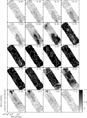
Figure 13: CO J=3-2 velocity channel maps of the MMS126 outflow. The greyscale is tailored to emphasize the low surface brightness outflow lobes. The contours are spaced by 1 K.

Table 1: Physical properties of the MMS126 molecular outflow. The values given in parentheses have been corrected for optical depth (assuming $\tau_{\rm CO}/(1-e^{-\tau_{\rm CO}})=3.5$) and inclination (assuming $i=57.3^{\circ}$).

	Blue		Red		Total
Maximum velocity (km/s)	6	(11.1)	7	(13)
Size (AU/pc)	20500/0.10	(24400)/(0.12)	19500/0.095	(23200)/(0.11)
Mass ($\times 10^{-4}$M⊙)	1.6	(5.5)	8.1	(28.2)	9.6	(33.7)
Dynamical timescale ($\times 10^{3}$ years)	16.2	(10.4)	15.4	(9.9)
Momentum ($\times 10^{3}$ M⊙ km/s)	5.4	(35)	25.6	(166)	31.0	(201)
Momentum flux($\times 10^{-8}$ M⊙ km/s y-1)	3.3	(34)	15.8	(160)	19.1	(193)
Kinetic Energy ($\times 10^{-3}$ M⊙ (km/s)2)	0.98	(12)	4.6	(55)	5.6	(67)
Mechanical luminosity ($\times 10^{-5}$L⊙)	1.0	(19)	4.9	(92)	5.9	(110)

MMS126 is a compact but resolved source forming part of a roughly east-west oriented, filamentary structure. It appears to coincide with a faint, cold IRAS source (IRAS~16253$-$2429: F12: $<$0.25 Jy; F25: $<$0.42 Jy; F60: 2.91 Jy; F100: 16.34 Jy). Close inspection of the HIRES processed IRAS maps reveals a faint source at 25$\mu$m, which however coincides with the nearby MMS060 = WSB~60. This latter source is also detected by ISO at 7 and 14 $\mu$m (Bontemps et al. 2001) but no clear source is seen at the position of MMS126. Finally, MMS126 appears to be driving a collimated near-IR H₂ outflow (Khanzadyan et al. 2004) and a molecular (CO) outflow (see Sect. 7.1 below).

Taking these arguments together (apparently cold FIR to millimetre source, no clear counterpart at wavelengths shorter than 25$\mu$m, and association with an outflow) we conclude that MMS126 is a very young stellar object, possibly still in the Class 0 phase. MMS126 would then be the second Class 0 object found in the $\rho$-Oph main cloud besides the prototypical source VLA1623 (Andre et al. 1993) but is of significantly smaller mass: using Eqn. 1, we derive a circumstellar dust mass of about 0.2 M_⊙ (VLA1623: 0.6 M_⊙, this work; Andre et al. (1993)).

7.1 The CO outflow

We observed the area around MMS126 in the CO(3-2) line using the JCMT on June 17 & 30 and on July 30, 2005. We took two position switched on-the-fly maps centered on MMS126, each covering a 80″$\times$180″ field at a position angle of 32^∘, sampling every 5″ with a 5″ spacing between rows. Smaller maps were added towards the end of the outflow lobes. The integration time on each point was 4 sec. The weather was good, with a stable atmosphere and $\tau_{230\leavevmode\nobreak\ {\rm GHz}}\sim 0.055$ (June 17), $\sim 0.08$ (June 30), and $\sim 0.045$ (July 30). In addition, spectra in frequency-switched mode were taken towards the position-switch OFF position. The spectra were baseline-subtracted, resampled to 0.6 km/s resolution, the OFF-position spectrum added, and finally gridded into one datacube within CLASS.

Figure 13 shows the resulting channel maps. Along the outflow axis indicated by our near-infrared H₂ observations there is clear evidence for a CO flow. Red-shifted emission is seen towards the south-west and some blue-shifted emission towards the north-east. Overall, the range over which higher-velocity gas is seen is fairly narrow. In the south-western, red-shifted lobe, it extends over a few velocity bins from about 5.7 to 8.5 km/s. Reasonably bright emission in the north-eastern, blue-shifted lobe is only seen in its tip, otherwise it is hardly separated and only faintly seen in two channels around 0 km/s; the contours in the velocity bins around 1 km/s indicate that this lobe contributes significantly at these velocities too, but is diluted by ambient emission. Outflow emission extends over about 2$\aas@@fstack{\prime}$5 (20000 AU/0.1 pc) out to the edges of the map, with both lobes showing a somewhat brighter, compact CO blob there, which might well be a terminating working surface; H₂ emission is also seen out to a similar distance in the south-western lobe.

We have derived estimates of basic flow properties as follows: the measured brightness temperature was converted to molecular gas column densities assuming the CO to be optically thin and in LTE at a temperature of 30 K; the CO abundance was assumed to be $10^{-4}$ of the H₂ abundance. Masses were derived as a function of velocity for each 0.6 km/s wide channel. Kinetic energies and momenta were derived as $E_{\rm kin}=1/2\sum M(v)\cdot(v-v_{\rm cen})^{2}$ and $P=\sum M(v)\cdot(v-v_{\rm cen})$, with $v_{\rm cen}=3.4$ km/s. A characteristic timescale was derived by dividing the maximum distance at which high-velocity emission was seen by the maximum CO velocity observed. The south-western, red-shifted lobe is seen to extend to the edge of the mapped area, so a maximum distance of 90″ was used; the north-eastern, blueshifted lobe seems to terminate within the mapped area. Finally, mechanical luminosities and momentum input rates were determined by dividing the total kinetic energy and momentum by the characteristic timescale.

Table 1 gives a list of outflow properties, for the blue- and red-shifted lobes alone and for the entire outflow. In parentheses we also list the outflow parameters after applying corrections for optical depth effects and inclination, following Bontemps et al. (1996) (assuming $\tau_{\rm CO}/(1-e^{-\tau_{\rm CO}})=3.5$ and an inclination $i=57.3^{\circ}$). The red- and blue-shifted emission does not seem to overlap, indicating that the flow axis is neither very close to the plane of the sky nor very nearly perpendicular to it, so $i=57.3^{\circ}$ might in fact be a reasonable assumption.

A comparison with the outflow parameters listed in Bontemps et al. (1996) shows that the MMS126 molecular outflow is one of the less energetic flows, as could be anticipated by the poor contrast of the flow against the ambient cloud material even in the CO(3-2) line and its fairly narrow extent in velocity space. Its momentum flux rate is much more typical for a more evolved object than for a Class 0 protostar. However, our map shows the flow to be fairly well collimated, which is more typical for the very youngest molecular outflows. Along with the deeply embedded, low circumstellar mass, low-luminosity nature of the driving source, the more likely explanation for the low energy/momentum input rate to the flow seems to be a very low protostellar mass (and age) rather than MMS126 being a relatively mature object at the end of the accretion and outflow phase.

8 Summary & Conclusions

We have performed a 1.2 millimetre survey of the main body of the $ρ$ Ophiuchi star-forming cloud. Our one square degree field enables us to verify and extend the results from previous surveys (MAN98 and J00). We detect and measure 143 cores, including 111 with no detected stellar objects. We identify a core, MMS126, which appears to harbour a new low-mass Class 0 protostar, driving a CO molecular outflow.

By comparing core masses with their sizes (as measured by the flux and FWHMs), we find that the cores contained within an inner circle of 0.2^∘ are compacter. This implies they are generally denser and of higher pressure. However, on comparison to the surface pressure required for hydrostatic equilibrium, there appear to be vast pressure variations (by a factor 10 to 100) within each location.

The data indicate that the mean core mass increases with the core radius. This can be measured despite the expected lower bound to the core masses given by the observational sensitivity (which would tend to distort the relation towards the form $\log{\rm M}\propto\log{\rm R}_{c}$) and despite the very wide range in possible core masses at each radius.

The clustering has also been investigated by deriving the two-point correlation function. We confirm previous results that the cores are highly clustered, similar to that of galaxy clusters (J00). However, from the two-point correlation function, we find no evidence for a critical length to identify with a Jeans length. However, the frequency of nearest neighbours provides a more local measure and reveals an abundance of small cores with low separation (5000 AU) – of order of the mean core size. This suggests that larger cores may fragment on this scale.

Moreover, the relevant velocity dispersion (in place of the sound speed) will also vary across the cloud, possibly producing velocity variations positively correlated with separation. Therefore, although the Jeans length remains a relevant length scale in turbulent fragmentation and collapse theory, an extended power-law correlation function could still be expected in a turbulent environment.

The cores are not distributed isotropically. There is a strongly preferred direction, transverse to the direction of the Sco OB association. However, the orientations of the major axes of the individual cores are consistent with a random distribution (§B, online version only).

The mass function may be approximated by a broken power law. As previously noted by MAN98 for the inner regions, this is similar to that of the galactic field IMF for stars. The flattening at lower masses occurs at a mass of $\sim$0.1 to 0.3 M_⊙, about twice as high as the equivalent break mass found for stars. We suggest that this difference is consistent with the core mass loss expected during the star formation process although the absolute value of the break is sensitive to assumed mass conversion parameters. An upper break at $\sim$0.5 – 1.0 M_⊙ is also found. A smoothly changing function such as a log-normal might be better suited to describe the core mass function derived from our observations, similar to the mass functions derived from numerical models of turbulence driven clouds by Ballesteros-Paredes et al. (2005).

The core mass function does not vary with position. That is, there is no evidence for a general mass segregation although the few highest core masses are found in the inner crowded zone.

How have the cores in L1688 developed? Turbulent motions are inherent to the entire clumps (Loren et al. 1990) and (although subsonic) also to the cores (Belloche et al. 2001). We may thus expect supersonic turbulence to drive high pressure and density variations on the scale of the cloud and clumps. Some density peaks within the chaotic flow may involve sufficient mass to become gravitationally bound; Elmegreen & Shadmehri (2003) argue that this scenario is the most likely one of the three they consider to have produced the millimetre continuum sources in Ophiuchus. The turbulence then decays within these proto-cores although it is still sufficient to generate molecular line profiles and contribute to core support in the observed cores (Belloche et al. 2001). As found in numerical simulations, the structure of these dynamical cores may closely resemble hydrostatic, gravitationally bound objects (Ballesteros-Paredes et al. 2003); they should also possess prominent infall signatures as indeed are found in several starless cores (Belloche et al. 2001). Furthermore, it is very likely that the detected cores are biased towards the slowest evolving long-lived objects. That is, the cores we actually observe are not typical of those which form but are simply a particular subset of cores which evolve very slowly, perhaps not even prone to collapse into stars.

The present study is consistent with a supersonic turbulence interpretation through the wide range in pressures, the hierarchical clustering and the randomness in core orientations, and the shape of the mass function. Turbulence, however, is generally supposed to be a means of dynamical support and rapid dispersal rather than quiescent confinement of equilibrium core configurations. If the clouds are close to equilibrium, the linear mass-radius relation would correspond to a fixed velocity dispersion. This indicates that a transition to coherence has already taken place and is a sign that the H₂ velocity dispersion is transonic or subsonic in the cores (Goodman et al. 1998). In recent hydrodynamic gravoturbulent simulations (Klessen et al. 2005), the majority of cores are actually found to be coherent and 80% are subsonic or transonic. The cores are produced behind shock waves, at stagnation points in converging turbulent flows. However, starless cores are also found to be gravitationally unbound in these simulations. This should in the future be tested by measurement of the virial masses of a large sample of the starless cores.

Further implications of the above results will be explored in a following work in which we relate the millimetre properties to those of the infrared and optical outflows from protostars and young stars. In combination with molecular spectroscopic studies of the cores, we will be able to constrain models for star formation in $\rho$ Ophiuchus.

Appendix A Notes on individual objects

available as jpg: 0511093.1331fa01.jpg
full postscript version available at http://www.ifa.hawaii.edu//users/stanke/preprints.html

Figure 14: The location, size, and orientation of the 143 millimetre sources identified from our survey.

Figure 15: The location, size, and orientation of the millimetre sources in and around the molecular clump A.

Figure 16: The location, size, and orientation of the millimetre sources in and around the molecular clump B.

available as jpg: 0511093.1331fa04.jpg
full postscript version available at http://www.ifa.hawaii.edu//users/stanke/preprints.html

Figure 17: The location, size, and orientation of the millimetre sources in and around the molecular clumps C, E, and F.

In this section we present a list of sources identified from our survey (Tab. 2), along with finding charts (Figs. 14, 15, 16, and 17) and short notes on the properties of individual sources, such as the presence of optical or near-infrared (stellar) counterparts, or whether absorption features as seen on the DSS or 2MASS images can be associated.

Table 2: List of 1.2 mm sources found in our survey. The sources are listed in the order they were identified by the wavelet decomposition plus clumpfind technique. F_int gives the integrated source flux in mJy; F_peak (a), (b), (c), and (d) give the peak fluxes determined in the following ways: (a): the maximum pixel value inside an ellipse defined by the minor and major axes of a gauss-fit to the source; (b): as above, but using only the wavelet scales from where on the source is detected first (given in parenthesis); (c): the peak flux after re-binning according to the source minor axis (see Sect. 3 for details); (d): the peak flux of the composite Gaussian model for the source. The columns labelled maj and min give the major and minor axis of a single Gaussian fit to the source (in arcseconds). PA gives the position angle of the source major axis in degrees east of north. The columns labelled as MAN98 and J00 give cross-identifications to the sources identified by Motte et al. (1998) and Johnstone et al. (2000), respectively. A long dash means that the source is outside the respective survey area, and “n.i.” labels features which are visible in the respective survey, but not identified as a separate feature. Cross-identifications given in parentheses mean that a feature found here is a part of a feature noted by MAN98 or J00. Finally, a comment on association with known YSOs is given. Apparently starless features are marked as “sl”.

	RA	DEC	Fint	Fpeak (mJy)				FWHM (″)		PA	MAN98	J00	Comment
	J2000	J2000	(mJy)	(a)	(b)	(c)	(d)	maj	min
MMS001	16:26:27.2	-24:23:46	7775	1999	1999 (1)	1828	2002	65	33	-7	SM1, SM1N	16264-2423	sl (SM1, SM1N)
MMS002	16:26:26.2	-24:24:28	1205	924	924 (1)	864	912	29	27	85	VLA1623	16264-2424	YSO: VLA1623 Class 0
MMS003	16:26:24.0	-24:16:12	242	248	248 (1)	227	251	26	24	-28	—	16264-2416	YSO: YLW32 opt/IR TTS
MMS004	16:26:30.4	-24:24:31	10255	973	973 (1)	912	987	95	57	-63	SM2	n.i.	sl
MMS005	16:26:21.3	-24:22:48	1060	357	357 (1)	320	351	50	35	-29	LFAM1	16263-2422	YSO: LFAM1; Class I?
MMS006	16:26:44.9	-24:23:06	291	230	230 (1)	217	226	28	24	6	—	16267-2423	YSO: GSS39 IR star Class I?
MMS007	16:26:28.3	-24:22:45	3137	490	490 (1)	425	482	77	51	-41	A-MM6/7	n.i.	sl
MMS008	16:26:58.4	-24:45:36	228	145	145 (1)	133	153	30	24	59	—	16269-2445	YSO: SR24 TTS binary
MMS009	16:27:09.1	-24:37:25	316	154	154 (1)	129	158	34	30	-1	Elia 2-29	16271-2437b	YSO:Elia 2-29
MMS010	16:26:23.7	-24:43:12	153	132	132 (1)	119	142	26	25	-32	—	—	YSO: YLW34 TTS
MMS011	16:27:27.3	-24:40:55	967	193	193 (1)	138	193	82	58	79	IRS43	16274-2440	YSO: WLY 2-43 Class I
MMS012	16:26:43.8	-24:17:22	1109	205	205 (1)	170	201	73	55	43	—	16267-2417	sl
MMS013	16:26:10.3	-24:20:52	84	70	70 (1)	70	78	26	19	62	GSS26	16261-2420	YSO: GSS26 Class I?
MMS014	16:26:22.5	-24:23:48	964	265	265 (1)	254	261	67	32	-19	A-MM1/2/3	n.i.	sl
MMS015	16:27:29.6	-24:27:37	1336	284	284 (1)	246	283	56	51	-46	B2-MM10	16274-2427c	YSO: VSSG17 (Class I?)
MMS016	16:27:27.8	-24:27:13	1058	236	236 (1)	220	240	75	36	63	B2-MM8	(16274-2427b)	YSO: contains NIR YSO VSSG18
MMS017	16:26:30.8	-24:22: 2	1145	187	187 (1)	163	202	101	43	35	n.i.	n.i.	sl
MMS018	16:27:33.5	-24:26:19	2900	350	350 (1)	307	333	78	66	-77	B2-MM16/17	16275-2426	sl
MMS019	16:26:18.7	-24:28:18	60	76	76 (1)	76	76	27	21	8	—	16263-2428	YSO: YLW31 Class II?
MMS020	16:27:13.0	-24:29:55	1150	152	152 (1)	126	155	92	66	32	B1-MM3	(16272-2429)	sl
MMS021	16:27:33.3	-24:27:32	718	130	130 (1)	110	125	98	44	-9	B2-MM15	n.i.	sl
MMS022	16:26:58.6	-24:34:06	4181	291	291 (1)	242	277	112	81	38	(C-S)	(16269-2434)	sl
MMS023	16:27:16.1	-24:31:13	186	83	83 (1)	78	78	41	31	23	B1-MM4	(16272-2430)	sl
MMS024	16:26:23.2	-24:24:43	274	127	127 (1)	104	101	46	35	23	LFAM3	n.i.	YSO: LFAM3 Class I ?
MMS025	16:26:43.3	-24:34:50	415	117	117 (1)	74	117	109	68	74	WL12	16267-2434	YSO: WL12
MMS026	16:26:23.2	-24:22:04	601	170	170 (1)	161	176	72	28	25	A-MM4	16264-2421	sl
MMS027	16:27:15.4	-24:30:34	1651	218	218 (1)	190	207	73	72	-39	(B1)	(16272-2430)	sl
MMS028	16:27:11.6	-24:29:15	874	176	176 (1)	151	161	67	50	2	B1-MM2	(16272-2429)	sl
MMS029	16:27:28.9	-24:26:39	610	225	225 (1)	208	238	49	30	76	B2-MM9/12	(16274-2427b)	sl
MMS030	16:26:08.0	-24:20:20	2614	146	146 (1)	111	153	142	92	10	Oph-A3	16261-2419	sl
MMS031	16:27:24.2	-24:27:42	1318	194	194 (1)	174	189	88	49	39	B2-MM3/4/5	(16274-2427a)	sl
MMS032	16:26:40.4	-24:27:13	114	83	83 (1)	72	85	33	28	-58	CRBR42	16266-2427	YSO: CRBR42 Class I?
MMS033	16:27:20.1	-24:27:09	624	138	138 (1)	124	123	76	38	45	B2-MM2	16273-2427	sl
MMS034	16:26:17.0	-24:23:40	126	70	70 (1)	67	69	26	24	-7	CRBR12	n.i.	YSO: CRBR12 Class I?
MMS035	16:27:23.8	-24:40:54	921	167	167 (1)	136	161	65	64	36	CRBR85 + F-MM2	n.i.	YSO: Class I (?)

Table 3: List of 1.2 mm sources found in our survey.

	RA	DEC	Fint	Fpeak (mJy)				FWHM (″)		PA	MAN98	J00	Comment
	J2000	J2000	(mJy)	(a)	(b)	(c)	(d)	maj	min
MMS036	16:27: 4.9	-24:39:09	1741	179	179 (1)	162	177	110	70	-79	E-MM2	16270-2439	sl
MMS037	16:27:25.5	-24:26:48	1721	248	218 (2)	224	241	77	55	55	B2-MM6	(16274-2427a)	sl
MMS038	16:27:58.6	-24:33:34	595	135	115 (2)	122	126	64	41	-13	—	—	sl
MMS039	16:27: 2.0	-24:34:46	1115	155	138 (2)	136	157	75	59	-68	(C-S)	(16269-2434)	sl
MMS040	16:27:21.1	-24:39:57	1725	199	177 (2)	169	183	87	64	-44	F-MM1, CRBR72	16273-2439	YSO: Class I
MMS041	16:28:58.7	-24:20:49	2827	164	149 (2)	142	159	150	86	-89	—	—	sl
MMS042	16:27:05.4	-24:36:34	433	115	86 (2)	90	105	68	43	-62	LFAM26	16270-2436	YSO
MMS043	16:27:10.1	-24:19:13	69	66	47 (2)	62	74	29	24	11	SR21	—	YSO: SR21
MMS044	16:26:59.1	-24:31:26	2212	149	135 (2)	116	138	122	91	-49	C-N	16269-2431	sl
MMS045	16:27:27.4	-24:39:26	576	106	88 (2)	88	107	79	54	-84	IRS44/46; CRBR88	16274-2439	YSO: IRS44/46; CRBR88
MMS046	16:26:10.5	-24:23:04	104	70	52 (2)	62	70	53	28	53	A3-MM1	16261-2423	sl
MMS047	16:28:29.4	-24:19:17	766	107	96 (2)	97	103	75	56	13	D-MM1/2	—	sl
MMS048	16:26:36.3	-24:17:52	863	122	107 (2)	107	129	86	70	-36	—	16265-2418	sl
MMS049	16:27:11.8	-24:27:37	511	113	94 (2)	93	88	86	53	83	B1B2-MM1	16271-2427	sl
MMS050	16:26:25.3	-24:22:19	709	154	132 (2)	144	153	78	39	19	A-MM5	16264-2422a	sl
MMS051	16:28:00.6	-24:32:54	548	104	90 (2)	95	105	74	46	-34	—	—	sl
MMS052	16:28:32.7	-24:17:50	1584	104	88 (2)	84	96	118	83	31	D-MM3/4/5	—	sl
MMS053	16:26:42.4	-24:26:02	210	79	64 (2)	63	76	64	43	-10	A-S	n.i.	sl
MMS054	16:26:32.8	-24:26:21	1479	136	116 (2)	116	123	109	74	-38	n.i.	16265-2426	sl
MMS055	16:26:48.2	-24:33:01	4527	120	104 (2)	90	111	180	140	3	C-W	n.i.	sl
MMS056	16:27:17.6	-24:27:37	648	91	80 (2)	81	89	81	70	-13	B2-MM1	16272-2427	sl
MMS057	16:26:11.9	-24:24:48	394	87	71 (2)	69	69	67	57	-65	A2-MM1	16261-2424	sl
MMS058	16:27:39.5	-24:39:16	39	48	29 (2)	41	51	28	24	-81	—	16276-2439	YSO: WSB52
MMS059	16:26:52.9	-24:34:45	603	99	86 (2)	88	82	72	62	-17	C-MM1	n.i.	sl
MMS060	16:28:17.1	-24:36:51	103	56	37 (2)	51	53	39	26	42	—	—	YSO: Class II (?)
MMS061	16:27:19.1	-24:28:46	375	83	71 (2)	75	78	57	47	53	B1B2-MM2	n.i.	YSOs: WL3/WL4/WL5/IRS37 Class II …
MMS062	16:27:06.4	-24:37:11	124	87	56 (2)	82	80	32	26	-4	E-MM3	16271-2437a	YSO
MMS063	16:26:14.6	-24:25:15	278	77	59 (2)	61	70	58	49	34	(A2)	(16262-2425)	sl
MMS064	16:27:39.7	-24:43:08	124	60	39 (2)	49	63	50	35	-52	IRS51	16276-2443	YSO: Class I WLY 2-51
MMS065	16:26:12.6	-24:20:13	120	64	45 (2)	59	51	42	34	-54	n.i.	n.i.	sl
MMS066	16:27:08.6	-24:28:30	447	83	65 (2)	66	70	85	43	-11	B1-MM1	n.i.	sl
MMS067	16:27:11.2	-24:39:26	227	63	49 (2)	55	60	51	42	-44	E-MM4	16271-2439	sl
MMS068	16:26:55.1	-24:38:10	693	65	51 (2)	52	54	145	71	-81	n.i.	n.i.	sl
MMS069	16:26:17.9	-24:25:22	128	59	45 (2)	49	51	55	31	52	(A2)	(16262-2425)	sl
MMS070	16:27:52.7	-24:31:43	340	67	47 (2)	44	53	143	52	-22	—	n.i.	core + YSO WLY 2-54
MMS071	16:27:11.8	-24:38:03	582	102	89 (2)	93	99	94	56	-57	E-MM5; WL20	16271-2437c, 16272-2438	YSO: includes WL20
MMS072	16:27:39.1	-24:26:57	337	71	59 (2)	62	69	64	49	39	n.i.	n.i.	sl
MMS073	16:27:40.2	-24:42:34	1272	86	75 (2)	74	73	172	67	-79	n.i.	16276-2442, 16277-2442	sl
MMS074	16:26:23.2	-24:20:45	452	54	43 (2)	44	44	173	37	-12	A-N & GSS31	16263-2419b, 16263-2419a	sl

Table 4: List of 1.2 mm sources found in our survey.

	RA	DEC	Fint	Fpeak (mJy)				FWHM (″)		PA	MAN98	J00	Comment
	J2000	J2000	(mJy)	(a)	(b)	(c)	(d)	maj	min
MMS075	16:29:01.4	-24:21:11	37	38	25 (2)	38	45	42	18	14	—	—	sl
MMS076	16:25:56.3	-24:20:48	102	42	30 (2)	34	38	33	27	37	—	16259-2420	YSO: TTS HBC259 Class II?
MMS077	16:26:49.0	-24:26:55	167	48	38 (2)	43	40	77	41	61	Oph-AC2	n.i.	sl
MMS078	16:27:39.9	-24:29:26	42	43	24 (2)	35	37	27	26	-9	n.i.	n.i.	sl
MMS079	16:26:33.4	-24:18:17	355	73	56 (2)	60	62	93	43	-21	—	n.i.	sl
MMS080	16:27:30.5	-24:41:56	779	77	67 (2)	60	80	96	80	-33	n.i.	n.i.	sl
MMS081	16:27:48.3	-24:44:44	588	66	51 (2)	45	55	128	65	87	—	16277-2444a, 16277-2444b	sl
MMS082	16:26:55.8	-24:36:44	338	47	34 (2)	43	40	167	33	69	$\sim$E-MM1	n.i.	sl
MMS083	16:27:38.2	-24:27:38	180	59	43 (2)	50	58	93	34	90	n.i.	n.i.	sl
MMS084	16:27:37.8	-24:46:05	894	63	44 (2)	40	46	200	85	-74	—	n.i.	sl
MMS085	16:26:30.4	-24:18:39	406	69	56 (2)	59	55	75	52	87	—	n.i.	sl
MMS086	16:27:19.1	-24:31:26	118	62	46 (2)	56	60	55	29	-7	(B1)	(16272-2430)	sl
MMS087	16:26:47.1	-24:29:28	1246	98	74 (3)	87	85	125	71	-39	Oph-AC2	16267-2429	sl
MMS088	16:25:58.6	-24:18:47	1786	88	64 (3)	69	65	259	90	-57	n.i.	n.i.	sl
MMS089	16:27:25.6	-24:33:32	640	56	38 (3)	44	46	90	73	-77	—	n.i.	sl
MMS090	16:27:01.8	-24:26:25	720	66	41 (3)	46	56	136	72	-89	n.i.	n.i.	sl
MMS091	16:25:58.8	-24:31:29	1392	81	45 (3)	41	41	178	146	-29	—	n.i.	sl
MMS092	16:29:19.5	-24:41:33	504	62	29 (3)	33	44	85	67	-46	—	—	sl
MMS093	16:27:43.6	-24:13:32	1759	74	46 (3)	44	46	176	111	-53	—	—	sl
MMS094	16:26:59.0	-24:22:59	1584	64	50 (3)	53	52	222	94	67	Oph-AB	n.i.	sl
MMS095	16:27:33.3	-24:15:40	992	56	37 (3)	38	46	177	115	-27	—	—	sl
MMS096	16:26:55.4	-24:19:14	545	51	34 (3)	38	37	146	90	42	Oph-G	16269-2419	sl
MMS097	16:28:14.2	-25:02:58	589	70	29 (3)	41	31	138	69	-19	—	—	sl
MMS098	16:25:47.3	-24:29:54	573	69	26 (3)	34	25	201	85	66	—	n.i.	sl
MMS099	16:28:07.4	-24:35:20	2658	64	46 (3)	45	55	283	125	-64	—	—	sl
MMS100	16:27:56.4	-24:42:48	637	47	28 (3)	36	34	212	64	82	—	—	sl
MMS101	16:27:12.7	-24:21:23	648	49	32 (3)	34	34	127	96	-88	—	—	sl
MMS102	16:29:07.7	-24:35:03	324	50	21 (3)	41	25	135	48	-88	—	—	sl
MMS103	16:27:55.2	-24:35:07	323	50	29 (3)	44	38	86	51	-75	—	—	sl
MMS104	16:26:27.9	-24:33:36	1166	65	41 (3)	42	46	141	119	-54	—	n.i.	sl
MMS105	16:25:44.6	-24:16:56	1068	55	32 (3)	32	31	191	131	49	—	n.i.	sl
MMS106	16:26:48.9	-24:23:33	169	39	25 (3)	36	38	64	50	49	n.i.	n.i.	sl
MMS107	16:27:40.3	-24:35:50	1488	57	39 (3)	44	40	277	104	-43	—	n.i.	sl
MMS108	16:27:20.6	-24:24:03	521	50	32 (3)	42	42	123	64	-19	(B3)	n.i.	sl
MMS109	16:29:11.2	-24:40:58	590	47	28 (3)	33	28	157	98	-75	—	—	sl
MMS110	16:25:49.4	-24:09:34	255	40	20 (3)	26	26	176	64	66	—	—	sl
MMS111	16:27:26.1	-24:36:21	180	34	19 (3)	29	26	111	53	68	—	n.i.	sl
MMS112	16:27:10.7	-24:26:15	273	49	28 (3)	40	38	95	50	28	n.i.	n.i.	sl
MMS113	16:26:34.3	-24:35:27	341	51	24 (3)	32	26	115	68	-58	—	n.i.	sl
MMS114	16:27:28.0	-24:20:32	223	40	21 (3)	29	26	88	58	59	—	—	sl
MMS115	16:26:16.2	-24:31:21	757	58	30 (3)	31	31	158	109	-76	—	n.i.	sl

Table 5: List of 1.2 mm sources found in our survey.

	RA	DEC	Fint	Fpeak (mJy)				FWHM (″)		PA	MAN98	J00	Comment
	J2000	J2000	(mJy)	(a)	(b)	(c)	(d)	maj	min
MMS116	16:29:01.7	-25:06:30	1214	76	37 (3)	38	39	181	132	-67	—	—	sl
MMS117	16:27:39.1	-24:41:15	315	49	31 (3)	43	43	71	54	82	n.i.	n.i.	sl
MMS118	16:27:15.1	-24:24:12	177	38	22 (3)	33	30	77	54	89	(B3)	n.i.	sl
MMS119	16:29:18.9	-24:35:46	248	50	20 (3)	24	27	80	73	17	—	—	sl
MMS120	16:28:54.3	-24:59:08	94	33	14 (3)	27	24	78	36	-54	—	—	sl
MMS121	16:26:04.1	-24:35:59	185	41	18 (3)	25	23	88	65	-78	—	n.i.	sl
MMS122	16:28:59.6	-24:41:08	244	43	20 (3)	27	24	91	75	24	—	—	sl
MMS123	16:26:17.3	-24:16:57	273	53	24 (3)	24	29	138	99	73	—	n.i.	sl
MMS124	16:26:37.8	-24:13:51	113	29	17 (3)	22	23	95	48	54	—	—	sl
MMS125	16:27:27.2	-24:16:56	209	37	21 (3)	29	28	96	52	-24	—	—	sl
MMS126	16:28:21.7	-24:36:21	411	121	121 (1)	102	118	53	43	21	—	—	YSO: IRAS 16253-2429, Class 0?
MMS127	16:26:44.4	-24:12:25	448	42	21 (3)	21	20	125	89	-66	—	—	sl
MMS128	16:29:17.8	-24:10:49	977	64	22 (4)	30	30	148	125	10	—	—	sl
MMS129	16:29:08.8	-24:13:55	1165	75	23 (4)	24	28	192	163	-67	—	—	sl
MMS130	16:28:34.4	-24:36:28	823	44	20 (4)	28	26	233	98	89	—	—	sl
MMS131	16:28:33.4	-25:03:19	958	48	20 (4)	25	22	238	142	30	—	—	sl
MMS132	16:27:00.1	-25:00:22	952	70	16 (4)	28	18	306	123	-53	—	—	sl
MMS133	16:29:05.9	-24:58:37	879	44	15 (4)	20	15	307	159	65	—	—	sl
MMS134	16:25:33.6	-24:35:03	426	49	13 (4)	17	17	161	124	43	—	n.i.	sl
MMS135	16:27:12.9	-24:50:02	234	32	10 (4)	19	15	148	86	-51	—	—	sl
MMS136	16:27:53.2	-24:26:13	531	37	12 (4)	19	17	168	103	35	—	—	sl
MMS137	16:27:57.7	-24:11:00	340	40	11 (4)	21	15	158	90	-83	—	—	sl
MMS138	16:28:58.5	-24:46:59	398	45	11 (4)	18	14	153	118	31	—	—	sl
MMS139	16:28:07.2	-24:59:55	770	53	12 (4)	17	16	168	122	-28	—	—	sl
MMS140	16:27:06.5	-24:38:10	144	62		54	54	55	26	-71	WL17	16271-2438	YSO: WL17
MMS141	16:25:38.0	-24:22:32	36	40		40	48	26	21	-9	—	16256-2422	YSO: Class I/II?
MMS142	16:27:17.2	-24:40:58	1058	83		68	67	133	66	-58	n.i.	n.i.	sl
MMS143	16:27:27.6	-24:24:38	342	53		42	36	100	51	-53	(B3)	n.i.	sl

MMS001: ridge NE of VLA1623: includes starless cores SM1 and SM1N; no optical/IR stellar counterpart.

MMS002: VLA1623 Class 0 (Andre et al. 1993); no opt/ir counterpart.

MMS003: pointlike source; optical/IR stellar counterpart YLW32.

MMS004: SM2 starless core; no opt/ir counterpart

MMS005: compact condensation in filament W of SM1/VLA1623 ridge; YSO LFAM1; no optical counterpart; bright NIR source, extended K-band nebula.

MMS006: pointlike source; GSS39/Elia2-27; no opt. coutnerpart; IR counterpart.

MMS007: part of filament extending NE of SM1/VLA1623; no clear opt/IR stellar counterpart.

MMS008: compact source: multiple T Tauri star SR24; the flux seems to be associated with the (so far) unresolved southern single component, as claimed by Nürnberger et al. (1998) and confirmed recently by Andrews & Williams (2005), rather than the northern (close binary) component. Our flux measurement is in good agreement with the result of Nürnberger et al. (1998).

MMS009: compact source; no opt. stellar counterpart; NIR star Elias 2-29 (also includes GY210).

MMS010: compact source; optical/IR counterpart YLW34

MMS011: compact source; YSO WLY 2-43; Class I; no opt. stellar counterpart; NIR star; high extinction.

MMS012: compact, but clearly extended source; SMM16267 of Wilson et al. (1999) (suggesting it to be a prestellar core) no optical counterpart; high extinction; fuzzy K band emission south of clump

MMS013: compact source; no opt. star; NIR star GSS26.

MMS014: elongated feature SE of MMS005; no optical counterpart; some IR stars might be associated. Breaks up into chain of three subcores in MAN98.

MMS015: bright compact core; no opt. stellar counterpart; NIR counterpart VSSG17; YSO; high opt. extinction.

MMS016: bright elongated core; YSO VSSG18 appears to be associated with this feature.

MMS017: part of filament extending NE of SM1/VLA1623; very faint K-band source at NE tip?

MMS018: compact core; no opt./NIR stellar counterpart.

MMS019: faint compact source; faint opt./bright NIR stellar counterpart YLW31

MMS020: bright core; no clear opt./NIR stellar counterpart; high opt. extinction.

MMS021: highly elongated; no opt./NIR stellar counterpart.

MMS022: bright large core; no opt./NIR stellar counterpart; high extinction.

MMS023: compact source; no clear optical counterpart; possibly IR star associated; high opt. extinction.

MMS024: LFAM3 faint opt., bright nebulous NIR source; visible on J00 map, but not noted as separate feature

MMS025: compact source (possibly surrounded by extended Halo); no opt. stellar counterpart; IR stellar counterpart WL12; high opt. extinction.

MMS026: elongated core NE of MMS005; no optical counterpart; faint K-band source?

MMS027: bright core; no clear opt./NIR stellar counterpart; possibly IR star to the SE associated; high opt. extinction.

MMS028: compact core; no clear opt./NIR stellar counterpart; high opt. extinction.

MMS029: elongated core. No opt./NIR stellar counterpart.

MMS030: extended core at SE tip of ridge (MMS088); no related optical feature.

MMS031: elongated core; no opt./NIR stellar counterpart.

MMS032: faint compact source; no optical counterpart; faint IR star CRBR42; ISO-Oph 54; [GY92] 91

MMS033: elongated core; no opt./NIR stellar counterpart.

MMS034: faint compact source; no optical counterpart; IR stellar counterpart CRBR12.

MMS035: compact source; no opt. stellar counterpart; NIR stellar counterpart, YSO CRBR85 Class I?; splits into two cores in MAN98 (YSO CRBR85 and F-MM2 starless core).

MMS036: no stellar counterpart for main core; MAN98 E-MM2b might have faint K-band counterpart.

MMS037: elongated core; no opt./NIR stellar counterpart.

MMS038: bright compact core; no opt./NIR stellar counterpart; high extinction.

MMS039: bright core adjacent to MMS022; no opt./NIR stellar counterpart; high extinction.

MMS040: elongated core; no opt./NIR stellar counterpart; high extinction. Contains MAN98 starless core F-MM1 and, at its north-western tip, the YSO CRBR72 (Class I).

MMS041: bright core; no opt./NIR stellar counterpart; near tip of cometary shaped high-optical-extinction cloud. The edge of the cloud are outlined by faint extensions to the east and west of this core.

MMS042: compact source; YSO LFAM26; no opt. stellar counterpart; faint K-Band source; optical extinction ridge.

MMS043: compact faint source, YSO SR21

MMS044: large core; compact source at center? no opt./NIR stellar counterpart; high extinction.

MMS045: faint compact core; no opt. stars; 3 NIR YSO stellar sources: IRS44/IRS46; CRBR88; 3 subsources det. by MAN98

MMS046: faint compact source; no clear opt/NIR counterpart.

MMS047: bright core; no opt./NIR stellar counterpart; at tip of cometary dark cloud.

MMS048: small core; no optical/NIR counterpart; high extinction. Part of small clump (together with MMS079 and MMS085).

MMS049: small faint core; no opt./NIR stellar counterpart; high opt. extinction.

MMS050: core in SM1 ridge; no clear opt/NIR stellar counterpart.

MMS051: compact core; no opt./NIR stellar counterpart; high extinction.

MMS052: rather bright elongated core; no opt./NIR stellar counterpart; tail of cometary dark cloud.

MMS053: small faint core; high optical extinction; no stellar opt./NIR counterpart.

MMS054: faint core; high optical extinction; no clear opt/IR stellar counterpart.

MMS055: faint core; no clear opt./NIR stars associated; high extinction.

MMS056: diffuse core; no opt./NIR stellar counterpart; high opt. extinction.

MMS057: small core; no clear optical/NIR counterpart. Part of small core (together with MMS063 and MMS069).

MMS058: faint compact source; YSO WSB52/LFAM p8/[GY92] 314; opt./NIR star.

MMS059: no opt./NIR stellar counterpart; high opt. extinction.

MMS060: faint compact source; opt/NIR stellar counterpart WSB~60 = BKLT~J162816$-$243657.

MMS061: elongated core; superposition of several NIR YSOs: WL3/WL4/WL5/IRS37; no optical stellar counterpart; high extinction. Class II sources. MAN98 classify this feature as composite pre-collapse core, but it might actually just be a superposition of circumstellar dust emission from the 4 NIR YSOs visible in this area.

MMS062: compact source; associated with edge-on disk YSO (Brandner et al. 2000).

MMS063: small core; no clear optical/NIR counterpart. Part of small clump (together with MMS057 and MMS069).

MMS064: faint compact source; no opt. star; NIR stellar counterpart; YSO: IRS51 = WLY 2-51 = YLW 45.

MMS065: faint compact source; seems to be associated with IR RN; YSO? hardly visible on MAN98 map; visible on J00 map, but not noted as separate feature.

MMS066: faint elongated core; no opt./NIR stellar counterpart; high opt. extinction.

MMS067: no opt./NIR stellar counterpart.

MMS068: extended core; no clear opt./IR stellar conterpart. There is emission visible in the MAN98 map, but there is some morphological difference from our and the J00 maps.

MMS069: small core; no clear optical/NIR counterpart. Part of small clump (together with MMS057 and MMS063).

MMS070: faint core; core + envelope structure? No opt. stellar counterpart; NIR star WLY 2-54.

MMS071: elongated core; no opt./NIR stellar counterpart; high extinction. Might split into a chain of faint sources. Includes NIR YSO WL20 at its south-eastern tip.

MMS072: faint core at eastern end of clump B2; no opt./NIR stellar counterpart.

MMS073: elongated core; no direct stellar counterpart, but [GY92] 301 is within core area.

MMS074: filament extending north of SM1 core; GSS31 on base of filament; possibly very faint nebulosity at tip.

MMS075: faint compact source nearby MMS041; no opt./NIR stellar counterpart.

MMS076: faint compact source; bright opt/NIR counterpart; V* V2058 Oph; HBC 259; SR4

MMS077: small faint core; located on high-extinction filament; no IR counterpart; not clearly visible in MAN98 map, part of their clump Oph-AC2

MMS078: faint small core, no opt./NIR counterpart.

MMS079: small core; no optical/NIR counterpart; high extinction. Part of small clump (together with MMS048 and MMS085).

MMS080: faint large core; no opt./NIR stellar counterpart.

MMS081: large, elongated core; 3 NIR (YSO?) stars on our around the core: GY344, GY370, GY352; high opt. extinction.

MMS082: faint filament; no opt/NIR stellar counterpart; high extinction. Corresponds roughly to MAN98 E-MM1, but differs in morphology from our and the J00 maps.

MMS083: faint core at eastern end of clump B2; no opt./NIR stellar counterpart.

MMS084: large core; no clear opt./NIR stellar counterpart; close to edge of high-extinction cloud; close to edge of J00 map; there is some emission, but it is not marked as separate feature.

MMS085: small core; no optical/NIR counterpart; high extinction. Part of small clump (together with MMS048 and MMS079).

MMS086: compact source; no clear opt./NIR counterpart; high opt. extinction.

MMS087: large core; no opt./NIR stellar counterpart; high extinction patch.

MMS088: SE-NW elongated ridge bounded by MMS030 and MMS105; apparently illuminated from the SW by HD147889 (SR1)

MMS089: faint extended core; no clear opt./NIR stellar counterpart; some bright NIR stars around; extinction patch.

MMS090: faint core; on optical extinction filament; no clear opt/IR stellar counterpart.

MMS091: faint large core; no stellar counterpart; optical extinction patch.

MMS092: faint core, no opt./NIR stellar counterpart; MMS092, MMS109, and MMS122 form a filament associated with high extinction.

MMS093: low surface brightness core; on high optical extinction lane (along with MMS095, MMS125, and MMS137); no clear opt/NIR stellar counterpart.

MMS094: part of larger ridge; no opt./IR stellar counterpart; on opt. extinction lane.

MMS095: low surface brightness core; on high optical extinction lane (along with MMS093, MMS125, and MMS137); no clear opt/NIR stellar counterpart.

MMS096: small low surface brightness core; no clearly associated optical/NIR counterpart.

MMS097: extended low surface brightness feature; no clear feature seen on DSS/2MASS.

MMS098: faint core; no stellar counterpart; optical extinction patch.

MMS099: ridgelike, elongated core; no opt./NIR stellar counterpart; high-extinction lane.

MMS100: large elongated core; no opt./NIR stellar counterpart; high extinction.

MMS101: part of larger ridge; on high optical extinction lane; no clear opt/NIR stellar counterpart; on edge of J00 map.

MMS102: very faint large core; no opt./NIR stellar counterpart; extinction patch.

MMS103: faint core; no opt./NIR stellar counterpart; high extinction.

MMS104: faint large core; no opt/NIR stellar counterpart; high-extinction.

MMS105: extended low surface brightness feature at NW end of ridge (MMS088); associated with diffuse K-band RN at SW edge; maybe some optical extiction patches associated.

MMS106: core on larger ridge; no opt./IR stellar counterpart; on opt. extinction lane.

MMS107: faint core; no clear opt./NIR stellar counterpart, but there are some IR stars in the core area which might belong to this feature; optical extinction filament.

MMS108/MMS118/MMS143: faint cores; no opt./NIR stellar counterpart; high optical extinction. part of MAN98 B3.

MMS109: faint core, no opt./NIR stellar counterpart; MMS092, MMS109, and MMS122 form a filament associated with high extinction.

MMS110: small faint core; small optical extinction whisps; IR star near peak position.

MMS111: faint core; no opt./NIR stellar counterpart; high extinction.

MMS112: faint core; no clear opt./NIR stellar counterpart; high opt. extinction lane?

MMS113: faint large core; possibly faint compact source also; no opt./NIR stellar counterpart; high-extinction lane.

MMS114: faint core; located on high optical extinction filament; no clear opt./NIR stellar counterpart.

MMS115: faint, large core; no opt./NIR stellar counterpart; high extinction lane.

MMS116/120: extended low surface brightness features; no clear features seen on DSS/2MASS.

MMS117: faint large core; no opt./NIR stellar counterpart; high extinction.

MMS118: see MMS108

MMS119: very faint large core; no opt./NIR stellar counterpart; extinction patch.

MMS120: see MMS116

MMS121: faint core; no stellar counterpart, roughly corresponds to optical extinction patch.

MMS122: faint core, no opt./NIR stellar counterpart; MMS092, MMS109, and MMS122 form a filament associated with high extinction.

MMS123: faint core; no optical counterpart; NIR star within core area; high extinction. Faint on J00 map.

MMS124: faint core, no opt./NIR stellar counterpart; high extinction.

MMS125: faint core; on high optical extinction lane (along with MMS093, MMS095, and MMS137); no clear opt/NIR stellar counterpart.

MMS126: compact source; no opt./NIR stellar counterpart; IRAS~16253$-$2429? Class 0? Main source might have a companion to the north-east.

MMS127: faint core; the YSO YLW37 (BKLT J162646-241203) is located at its north-eastern periphery.

MMS128: very faint large core; no opt./NIR stellar counterpart; extinction patch.

MMS129: very faint large core; no opt./NIR stellar counterpart; extinction patch.

MMS130: large, faint, elongated core; no opt./NIR star associated; extinction lane.

MMS131/132/133/139: extended low surface brightness features; no clear features seen on DSS/2MASS.

MMS134: low surface brightness; no opt. stellar counterpart, diffuse nebulosity; NIR star GSS15/BKLT J162535-243400 at north-eastern periphery. Faint stuff on J00 map.

MMS135: low surface brightness; small optical extinction patch.

MMS136: low surface brightness; 2 optical/NIR stars, V 2059 Oph and ISO-Oph 180 (Bontemps et al. 2001) within core area. On edge of MAN98 and J00 maps.

MMS137: low surface brightness; on high optical extinction lane (along with MMS093, MMS095, and MMS125); no clear opt/NIR stellar counterpart.

MMS138: low surface brightness; some opt./NIR stars visible at core periphery.

MMS139: see MMS131

MMS140: faint compact source plus more extended core; no opt. counterpart; NIR star WL17; high extinction.

MMS141: faint compact source; stellar NIR counterpart; optically very faint; Class I/II?

MMS142: faint extended core.

MMS143: see MMS108

Appendix B Orientation

On the largest scale, the $\rho$ Ophiuchi cloud possesses southeast-northwest ridges (general orientation of $\sim$ 145^∘) along with filamentary tails stretching in the NNE direction ($\sim$ 70^∘) over four degrees on the sky (Loren 1989a).

A preferred cloud direction on sub-degree scales is also apparent, as shown on our 1.2 mm image (Fig. 1). Here, we quantify this by determining the orientation between each pair of cores. The resulting number distribution is displayed in Fig. 18.

Figure 18: The number distribution of core-core orientations determined for each pair of cores (a total of 10,153 pairs; solid line), each pair separated by less than 30,000 AU (508 pairs; dotted line) and those separated by more than 30,000 AU (dashed line). The latter two distributions have been normalised so that the total number is constant (i.e. displaying equal areas under the lines).

Not surprisingly, the result is that the preferred core-pair direction is not only maintained on the sub-degree scale (solid line) but remains just as prominent below the separation of 30,000 AU (0.06^∘). Thus the preferred direction of $\sim$ 130 - 150^∘ corresponds to the ridge direction – the expected direction of compression from shocks transmitted from the Sco OB2 association (Vrba 1977; Loren 1989b).

Is the preferred direction still present on even smaller scales? To answer this, we plot the number distribution of the orientations of the major axis of each core in Fig. 19. We find no obvious trend in the data although the statistics are quite small. This result applies to the entire sample as well as the starless cores which implies that any preferred direction is lost at any early stage in core development.

Figure 19: The number distribution of orientations of the major axes of the 111 starless cores (upper panel) and the entire 143 cores (lower panel).

To further check for the presence of local (or global) alignment of core orientations, we have analysed the absolute difference in position angles ($\Delta$PA) that every core includes with its neighbours. Fig. 20 (upper panel) shows the average position angle difference of all cores with respect to their $n$’th nearest neighbour. The large scatter in $\Delta$PA around 45^∘ indicates that the large majority of cores is randomly oriented with respect to their neighbours. At most a tiny tendency towards lower average $\Delta$PA is seen for the few very next neighbours; the still large scatter indicates that this can only be due to very few cases showing some degree of alignment, while the great majority is randomly oriented.

Fig. 20 (lower panel) shows the average $\Delta$PA as a function of the projected distance from every core. Again, at most a very small trend towards smaller average $\Delta$PA at the smallest separations can be seen. The large scatter again indicates that this trend is caused by only a few core pairs, with most core pairs including random $\Delta$PA.

Figure 20: The relative orientation (difference in position angles) of core major axes with respect to their neighbours: average relative orientation with respect to the $n$th neighbour (upper panel), and average relative orientation of cores within a certain (projected) distance to the core. The smallest cores (with major axes determined to be smaller than 28″) have been omitted.

Thus it appears that there is virtually no tendency for alignment of core orientations, supporting the idea of core formation as a result of unordered, turbulent motions. In particular, supposing that the orientation of the core major axis is perpendicular to the direction of preferred contraction, this contradicts the idea of ordered magnetic fields as producing agent of aligned protostellar disk/jet systems.

Two (counteracting) effects should be kept in mind in the interpretation of this result: residual scanning effects might locally push measured core orientations towards a similar position angle. On the other hand, we only can analyse the projected core distribution; a core seen to be the nearest neighbour in this 2-D projection might in fact be at much larger distance in 3-D, which will tend to dilute any local alignment, thus in fact alignment might be more prevalent than seen here.