The Iron K-shell features of MXB~1728–34 from a Simultaneous Chandra-RXTE Observation

We report on a simultaneous Chandra and RossiXTE observation of the low-mass X-ray binary atoll bursting source MXB~1728–34 performed on 2002 March 3–5. We fit the 1.2–35 keV continuum spectrum with a blackbody plus a Comptonized component. Large residuals at 6–10 keV can be fitted by a broad (FWHM $\simeq 2$ keV) Gaussian emission line or, alternatively, by two absorption edges associated with lowly ionized iron and Fe XXV/XXVI at $\sim 7.1$ keV and $\sim 9$ keV, respectively. In this interpretation, we find no evidence of broad, or narrow, emission lines between 6 and 7 keV. We test our alternative modelling of the iron K shell region by reanalysing a previous BeppoSAX observation of MXB~1728–34, finding a general agreement with our new spectral model.

1 Introduction

MXB~1728–34 (discovered by Lewin et al. 1976; see also Hoffman et al. 1976) is a low-mass X-ray binary, a well known prototype of the class of the bursting atoll sources (Hasinger & van der Klis 1989). The distance to the source is estimated between 4.1 kpc and 5.1 kpc (Di Salvo et al. 2000, Galloway et al. 2003). This was one of the first sources to display kilohertz quasi-periodic oscillations (kHz QPOs) in its power spectrum and the first to display quasi-coherent oscillations, now identified as the spin frequency of the neutron star (NS), around 363 Hz, during some type I X-ray bursts (Strohmayer et al. 1996). Its temporal behaviour has been extensively studied by Di Salvo et al. (2001) and van Straaten et al. (2002), using a large set of RXTE observations, spanning more than three years.

Power spectra of NS systems show a variety of rapid X-ray variability components and noise features. Among the high-frequency phenomena kilohertz quasi-periodic oscillations (kHz QPOs) are the fastest variability components. Two QPO peaks usually occur in the range 200–1200 Hz, the higher frequency QPO denoted the upper kHz QPO, the other the lower kHz QPO; their frequencies move to higher values as the spectral state of the source changes, while the peak separation remains almost constant, probably being related to the spin frequency of the neutron star or to half its value (see e.g. van der Klis 2000). Neutron-star hectohertz QPO is a peaked noise component in the frequency range 100–200 Hz, which does not present any clear correlation with other features in the power spectrum but could be linked to the high-frequency QPOs observed in some black-hole systems (Nowak 2000). The low frequency complex is dominated by a broad band noise component, usually modelled with a zero-centered Lorentzian, and one or two broad QPOs in the range 0.1–50 Hz, usually denoted Low-Frequency QPO (LFQPO) and Very Low Frequency QPO (VLFQPO).

Spectral studies have been carried out in the past with the EXOSAT (White et al. 1986), RXTE (Piraino et al. 2000) and BeppoSAX (Di Salvo et al. 2000, Piraino et al. 2000) satellites. White et al. (1986) found that the continuum emission could be well described by a Comptonization model, and interpreted this result in the framework of the so called Western Model, where the majority of the X-ray emission is disk emission Comptonized in a sorrounding corona (but in bright sources a blackbody component, interpreted as emission from the NS surface was also modeled, see also White et al. 1988). Di Salvo et al. (2000) and Piraino et al. (2000) found that a two-component model was required to fit the broad energy band spectra of MXB~1728–34 from BeppoSAX (0.1–200 keV range) and RXTE (3.0–60 keV range). The spectra, in both cases, consisted of a soft component (a multicolor disk blackbody or a blackbody spectrum), probably produced by the disc, and a Comptonized spectrum, responsible for the hard emission, where seed photons arising from the neutron star, or from an optically thick boundary layer, are scattered by a small spherical corona placed between the innermost edge of the accretion disc and the neutron star surface (a description known in literature as the Eastern Model, Mitsuda et al. 1989). More recently, detailed and extensive studies on dipping X-ray sources (Bałucińska-Church et al. 1999, 2000, Church & Bałucińska-Church 2004) have shown that the size of the accretion disk corona (ADC, $\simeq$ 50,000 km) largely exceeds the inferred inner edge of the accretion disk, so that the majority of the disk emission is expected to be strongly Comptonized. The Birmingham Model, i.e. a blackbody emission from the NS plus a Comptonized emission from an extended accretion disk corona, therefore, seems now physically more appropriate in describing the continuum emission from LMXBs (see also Church & Balucińska-Church 2001). However, different interpretations of the dipping behaviour and the consequent continuum modelling are still debated (Boirin et al. 2005).

Part of the hard X-ray emission could evenually be scattered by the disc, producing Compton reflection features such as a broad Gaussian line at 6.4–6.7 keV. However, the width of the line inferred from the fits ($\geq$ 0.5 keV) lacks a clear physical interpretation, as up to date it is yet disputed how this width could actually arise (see also Asai et al. 2000 for a critical discussion on possible broadening mechanisms).

In this paper we present new results from a simultaneous Chandra-RXTE observation of MXB~1728–34. We propose an alternative fit of the iron K-shell region, using two absorption edges instead of a very broad emission line, the interpretation of which could be quite problematic.

2 Observations and Data Reduction

MXB~1728–34 was observed with Chandra from 2002 March 4 15:20:34 to 2002 March 5 00:27:26 using the High Energy Transmission Grating Spectrometer (HETGS). The data were collected in the Timed Exposure Mode, using a subarray of the ACIS-S cameras in order to mitigate the effects of photon pile-up in the first order spectra. Consequently the frame time was 1.44 s, the High Energy Grating (HEG) spectrum was cut-off below 1.6 keV and the Medium Energy Grating (MEG) spectrum below 1.2 keV. The RXTE observation started on 2002 March 3 03:27:12 and ended on 2002 March 5 13:00:00. We used only the Proportional Counter Array (PCA) data; the total available time, i.e. the time during which at least one Proportional Counter Unity (PCU) was on, was $\sim 97$ ks. For the timing analysis we used only PCU0 and PCU2, which are the PCUs with the longest simultaneous on-source time (almost 90 ks), while for the spectral analysis we used PCU2 and PCU3, avoiding the use of PCU0 because starting 2000 May 12 it suffered the loss of the veto propane layer. We used Standard2 configuration, with 16 s time resolution and 129 energy channels, for the spectral analysis and Event Mode configuration, with 128 $\mu s$ time resolution and 64 energy channels, for the temporal analysis.

We used the CIAO 3.0 software package for the reduction of the Chandra data, FTOOLS 5.3 for the reduction and analysis of the PCA data, and XSPEC v. 11.3 for the spectral analysis. Because the Rapid Burster is inside the field of view of the PCA ($\sim 1^{\circ}$) we checked the flux of this source during our observation analyzing the All Sky Monitor (ASM) lightcurve. We found that the source did not show any significant activity so that the associated flux should be less than $1.4\times 10^{-11}$ erg cm^-2 sec^-1 (Masetti et al. 2000). Because the flux of MXB~1728–34 in the same energy range during our observation was $\sim$ 1.5 $\times$ 10^-9 erg cm^-2 sec^-1, we concluded that the Rapid Burster contamination is absolutely negligible.
In order to constrain the systematic error for the PCA spectra we analyzed an observation of the Crab Nebula (Obs. ID 70018-01-01-00), performed 50 min after our observation of MXB~1728–34. We fitted the Crab spectrum with a simple photoelectrically absorbed power-law model and derived the systematic error from the residuals in the fit as described in Wilms et al. (1999), treating the spectra of different PCUs as independent datasets fitted under the same model. We raised the level of systematics until a value of $\chi^{2}\leavevmode\nobreak\ <\leavevmode\nobreak\ 2$ was obtained. These operations resulted in a 2% systematic error for channels below 25 keV, and 2.5% for the remaining channels.

Seven type-I bursts were revealed in the PCA lightcurve and two bursts in the Chandra lightcurve. As our primary concern is studying the persistent emission of the source we discarded data intervals centered around each burst, for a time length of 160 sec. The persistent flux of the source, during the whole observation, showed little variability, and remained at about 20–25 cts/s for the Chandra diffraction arms and 235–270 cts/s/PCU for the PCA, thus confirming that any contamination of the Rapid Burster can be safely neglected.

3 Temporal Analysis

We studied the Power Density Spectrum (PDS) of MXB~1728–34 using the high-time resolution data of the RXTE/PCA. The power spectra were constructed by dividing the PCA lightcurve, with no energy selection, into segments of 256 s and then binning the data in time before Fourier transforming such that the Nyquist frequency was 2048 Hz in all cases; the PDS were normalized according to Leahy et al. (1983). All the PDS produced were finally summed and averaged into a single PDS. The Poisson noise estimated in the frequency range between 1200 and 2048 Hz (where neither noise nor QPOs are known to be present) was subtracted before fitting.

A satisfactory fit of the PDS is obtained by decomposing the power spectrum into a sum of five Lorentzians (see e.g. Belloni et al. 2002): a zero-centered Lorentzian, which accounts for the band-limited noise component (BLN Lorentzian), a Lorentzian centered at $\simeq$ 23 Hz (the VLFQPO Lorentzian, L_VLF), a Lorentzian centered at $\simeq$ 38 Hz (the LFQPO Lorentzian, L_LF), a broad Lorentzian centered at $\simeq$ 130 Hz (the hectohertz QPO, L_hHz), and finally a Lorentzian at $\simeq$ 650 Hz (the kHz QPO, L_kHz). Parameters best-fit values and associated errors, calculated for $\Delta\chi^{2}=1.0$, equivalent to 1 $\sigma$ confidence level, for this fit are reported in Table 1.

It has been shown that the value of the centroid frequency of the kHz QPOs correlates well with the position of the source in the color-color diagram (CD), gradually increasing as the source moves from the Island State to the Banana State (e.g. van der Klis 2000). The average PDS during our observations looks similar to the PDS numbered 7 in Di Salvo et al. (2001) when the source lies in the lower part of its Island State. The high value of the rms fractional amplitude of the L_kHz detected during the Chandra-RXTE observation strongly suggests it is the upper peak of the twin kHz QPOs; following this identification, we find that the parameters of the other components obtained from our fit are in good agreement with the correlations shown in Di Salvo et al. (2001), except that we detect L_VLF, which van Straaten et al. (2002) argued could only appear as both the lower and the upper kHzQPOs were present. The presence of this feature during our observation may be linked to the frequency statistical resolution of the power spectra, as our integration time greatly exceeds the integration time used in past analyses. Integrating on shorter timescales ($\leq$ 20 ksec) we found that the VLFQPO was no longer required for a good fit. In this case, the best value of peak frequency of the LFQPO stayed almost constant at 23 Hz, while the value of the parameters of the other Lorentzians did not change significantly, so that our analysis would coherently agree with the previous ones.

Both the timing properties and the position of the source in the CD track suggest that during our observation MXB~1728–34 was in the Island State, corresponding to a relatively low, or intermediate, mass accretion rate.

Table 1: Results of the MXB~1728–34 PDS fit in the frequency range $3.9\times 10^{-3}-2048$ Hz. Here $\nu_{0}$ is the centroid frequency and $\Delta$ is full width at half maximum of each Lorentzian line. The root-mean-square amplitude (RMS) is calculated integrating each Lorentzian from 0 to infinity. Errors are quoted at $1\sigma$ confidence level.

Component	Parameter	Value
BLN	$\nu_{0}$ (Hz)	0 $(fixed)$
BLN	$\Delta$ (Hz)	20.9$\pm$0.4
BLN	RMS (%)	21.6$\pm$0.5
LVLF	$\nu_{0}$ (Hz)	23.2$\pm$0.3
LVLF	$\Delta$ (Hz)	11.5$\pm$1.5
LVLF	RMS (%)	6.0$\pm$0.8
LLF	$\nu_{0}$ (Hz)	38.1$\pm$1.7
LLF	$\Delta$ (Hz)	26.8$\pm$2.0
LLF	RMS (%)	7.0$\pm$0.7
LhHz	$\nu_{0}$ (Hz)	134$\pm$7
LhHz	$\Delta$ (Hz)	221$\pm$22
LhHz	RMS (%)	12.4$\pm$0.7
LkHz	$\nu_{0}$ (Hz)	647$\pm$5
LkHz	$\Delta$ (Hz)	175$\pm$8
LkHz	RMS (%)	10.4$\pm$0.7
$\chi^{2}$/dof		512/432

4 Spectral Analysis

For the Chandra/HETG data, we considered the four first-order dispersed spectra, namely the two HEG spectra and the two MEG spectra on opposite sides of the zeroth order image. We averaged HEG+1 (MEG+1) and HEG-1 (MEG-1) spectra into a single spectrum, after having tested their reciprocal consistency. We used data in the 1.6–10 keV range for the HEG spectrum and 1.2–5 keV range for the MEG spectrum. For all the fits we took into account an instrumental feature at 2.07 keV for bright sources, described by Miller et al. (2002), and fit it with an inverse edge (with optical depth $\tau\simeq-0.1$). The HEG and MEG spectra were binned in order to have at least 300 counts for each bin. This, however, still ensures a high number of channels (about 1000) and good spectral resolution throughout the entire covered energy band.

For the RXTE/PCA data we applied the standard selection criteria for obtaining good time intervals. We limited the analysis to the 3.5–35 keV energy range and applied a systematic error as described in §2.

We restricted the spectral analysis to the intervals during which RXTE operated simultaneously with Chandra. Relative normalizations of the three instruments, except for HEG which was fixed to a reference value of 1, were left as free parameters in all the fits.

We applied a series of models to simultaneously fit HEG, MEG, and RXTE spectra. Because in this paper we are interested in the study of discrete features, we used to describe the continuum the two-component model which gave the lowest value of $\chi^{2}$. We find the best-fit continuum model to consist of a soft component, described by a blackbody of temperature $kT_{bb}\leavevmode\nobreak\ \simeq$ 0.51 keV, plus a Comptonized component (CompTT in XSPEC; Titarchuk (1994)), with seed-photon temperature $kT_{0}\leavevmode\nobreak\ \simeq$ 1.3 keV, electron temperature $kT_{e}\leavevmode\nobreak\ \simeq$ 7.4 keV and optical depth, associated to a spherical corona, $\tau\leavevmode\nobreak\ \simeq$ 6.2. Both components are photoelectrically absorbed by an equivalent hydrogen column $N_{H}\simeq 2.6\times 10^{22}$ cm^-2. The $\chi^{2}$/dof obtained for this fit is 1206/1034.

An absorption feature, resembling an edge, at 1.84 keV, probably associated to neutral Si, is clearly visible in the MEG and HEG spectra (see Fig. 1, left panel). To fit this edge we substituted the absorption component phabs in XSPEC with the component vphabs, which allows us to vary the abundances of single elements with respect to the solar abundances. We find that a Si abundance $\sim$ 2 times larger than the solar abundance improves the fit significantly ($\chi^{2}$/dof = 1031/1033 for this fit).

With respect to any continuum model that we tried, large residuals in the 6–10 keV range are clearly visible (Fig. 1, left panel) and can be fitted by a very broad Gaussian emission line. Leaving the parameters of the line free gives, however, unphysical results (position of the line $\simeq$ 5.5 keV and $\sigma\simeq$ 1.5 keV). Confining the position of the line in the range 6.4–6.7 keV gives a line width $\sigma\simeq 1$ keV (equivalent width $\simeq 270$ eV); fixing the width of the line to 0.5 keV constrains its position at $\simeq 6.1$ keV. Alternatively, we can also fit these residuals with absorption edges, instead of emission lines, associated with lowly ionized iron and Fe XXV/XXVI at $7.03$ keV ($\tau\simeq 0.11$) and $\sim 9$ keV ($\tau\simeq 0.16$), respectively. The addition of these edges improves the fit significantly compared to the simple blackbody plus Comptonization model described above, giving $\chi^{2}$/dof of 959/1029. In this interpretation, we no longer find evidence of broad or narrow iron emission lines between 6 and 7 keV.

To test our model we reanalyzed a previous BeppoSAX observation performed between August 23 and 24, 1998 (see Di Salvo et al. 2000). During this observation the ASM lightcurve of the Rapid Burster showed that the source was in an active state (10.7/11.8 cts/s, one-day average). LECS and MECS spectra, which were extracted using circular regions around MXB~1728–34 of 8’ and 4’ radii respectively, are not affected by the contaminating source. HP and PDS spectra , extracted from a 1^∘ region, can be affected up to 10-15% for the source flux. The normalization constants among the MECS/LECS/PDS/HP instruments are inside the expected calibration ranges so that, although we cannot exclude some contamination in the residuls of our fits above 10 keV, our conclusions in the low energy band of the spectrum still hold.

We fittted the 0.12-60 keV BeppoSAX spectrum with the same continuum adopted for the Chandra-RXTE dataset. A Gaussian emission line is no longer required if we introduce two absorption edges at energies above 7 keV. In this case, we find the first edge at $\simeq$ 7.5 keV ($\tau$ $\simeq$ 0.08) and the second edge at $\simeq$ 8.8 keV ($\tau$ $\simeq$ 0.08). The BeppoSAX spectrum is in agreement with the Chandra-RXTE spectrum, giving a $\chi^{2}$/dof = 207/178, instead of $\chi^{2}$/dof = 235/180 obtained for the model adopted in Di Salvo et al. (2000)). Note that the overabundance of Si with respect to Solar abundance required to fit the Chandra-RXTE spectrum is not required to fit the BeppoSAX spectrum. On the other hand, the BeppoSAX spectrum shows in this energy band a prominent narrow emission line at 1.67 keV (Fig. 2, left panel), compatible with the radiative recombination emission from Mg XI (see Di Salvo et al. 2000). This feature, however, is not detected in the Chandra spectrum. Removing this emission line from the fit gives a worse $\chi^{2}$/dof but a Si-overabundance is required to fit the data, resulting in values also in agreement with the Chandra-RXTE dataset; in this case we find that $\chi^{2}$/dof is 225/179 when the Si abundance is $2\pm 0.5$ times solar, and $\chi^{2}$/dof is 247/180 when the Si abundance is fixed to the solar value.

The best-fit parameters for the fits of the Chandra-RXTE and BeppoSAX datasets are reported in 2; residuals in units of $\sigma$ with respect to the simple continuum model are shown in Figures 1 and 2 (left panels); data and residuals corresponding to the two edge model are shown in Figures 1 and 2 (right panels).

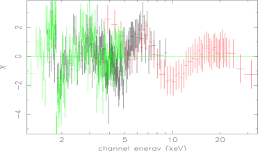
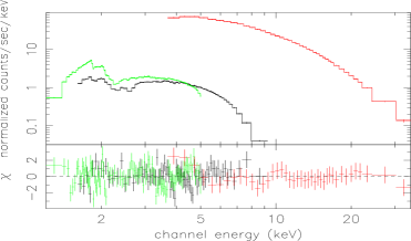
Figure 1: 1.2–35.0 keV spectra of MXB~1728–34 obtained from the simultaneous Chandra and RXTE datasets. Left panel: residuals in unit of $\sigma$ with respect to the absorbed blackbody plus CompTT model. Right upper panel: Chandra and RXTE /PCA spectra together with the two-edges model (see table 2) shown on top of the data as solid line; right lower panel: residuals to the best-fit model. Data have been rebinned for clarity: MEG data in green, HEG data in black, PCA data in red.

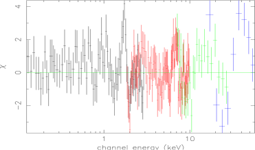
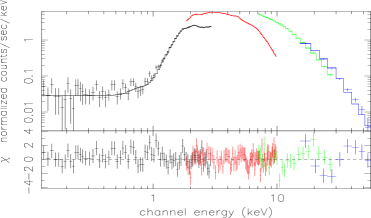
Figure 2: 0.12–60 keV spectra of MXB~1728–34 obtained from the BeppoSAX observation. Left panel: residuals in unit of $\sigma$ with respect to the absorbed blackbody plus CompTT model. Right upper panel: BeppoSAX spectra together with the two-edges model (see table 2) shown on top of the data as solid line; right lower panel: residuals to the best-fit model.

Table 2: Best fit parameters of MXB~1728–34 for the Chandra/RXTE spectra (1.2–35 keV) and the BeppoSAX spectra (0.12–60 keV energy band). The continuum emission consists of a blackbody (bbody) and a Comptonized component (compTT). $kT_{\rm BB}$ and N_BB are, respectively, the blackbody temperature and normalization in units of $L_{39}/D_{10}^{2}$, where $L_{39}$ is the luminosity in units of $10^{39}$ ergs/s and $D_{10}$ is the distance in units of 10 kpc. $kT_{0}$, $kT_{\rm e}$ and $\tau$ indicate the seed-photon temperature, the electron temperature, and the optical depth of the spherical Comptonizing cloud. N_CompTT is the normalization of the CompTT model in XSPEC v.11.3 units. Unabsorbed luminosities of the bbody component and of the CompTT component are calculated assuming a distance to the source of 5.1 kpc (Di Salvo et al. 2000) in the 0.1–100 keV energy range. For the edge components, E_edge denotes the energy of the edge and $\tau$ the optical depth. For the Gaussian component, E_Line is the line centroid energy, $\sigma$ the line width, and N_Gauss the total photons/cm²/s in the line. The position of the line at 1.66 keV had to be fixed in order to make stable the fit. Uncertainties are given at the 90% confidence level.

		Chandra-RXTE	Chandra-RXTE	BeppoSAX	BeppoSAX
		2 Edges	Broad Line	2 Edges	Broad Line
Component	Parameter (Units)	Values
vpha	$N_{\rm H}$ $(10^{22}$ cm${}^{-2})\dotfill$	$2.61^{+0.06}_{-0.07}$	$2.66^{+0.07}_{-0.07}$	$2.31^{+0.08}_{-0.07}$	$2.36^{+0.09}_{-0.08}$
vpha	Si (Solar units)	$2.02_{-0.13}^{+0.13}$	$1.95_{-0.12}^{+0.11}$	$\dots$	$\dots$
edge	Eedge(keV)	$7.03^{+0.08}_{-0.06}$	$\dots$	$7.47^{+0.14}_{-0.13}$	$\dots$
edge	$\tau$ $(10^{-2})$	$11^{+3}_{-4}$	$\dots$	$8^{+2}_{-2}$	$\dots$
edge	Eedge (keV)	$9.0^{+0.3}_{-0.4}$	$\dots$	$8.82^{+0.2}_{-0.19}$	$\dots$
edge	$\tau$ $(10^{-2})$	$16^{+4}_{-4}$	$\dots$	$8.82^{+0.2}_{-0.19}$	$\dots$
Gauss	ELine (keV)	$\dots$	$6.12^{+0.19}_{-0.19}$	$\dots$	$6.74^{+0.15}_{-0.15}$
Gauss	$\sigma$ (keV)	$\dots$	$0.5$ (fixed)	$\dots$	$0.5$ (fixed)
Gauss	NGauss $(10^{-3})$	$\dots$	$2.3^{+0.5}_{-0.5}$	$\dots$	$1.7^{+0.5}_{-0.5}$
Gauss	ELine (keV)	$\dots$	$\dots$	$1.66$ (fixed)	$1.66$ (fixed)
Gauss	$\sigma$ (keV)	$\dots$	$\dots$	$0^{+0.05}$	$0^{+0.05}$
Gauss	NGauss $(10^{-3})$	$\dots$	$\dots$	$11^{+3}_{-3}$	$11^{+0.3}_{-0.3}$
bbody	kT (keV)	$0.513_{-0.014}^{+0.014}$	$0.478_{-0.014}^{+0.014}$	$0.619_{-0.013}^{+0.013}$	$0.590_{-0.017}^{+0.017}$
bbody	NBB $(10^{-3})$	$10.7_{-0.4}^{+0.4}$	$10.1_{-0.5}^{+0.5}$	$19_{-5}^{+5}$	$18_{-0.5}^{+0.6}$
bbody	L $(10^{36}$ erg sec${}^{-1})$	2.78	2.60	4.96	4.69
CompTT	$kT_{0}$ (keV)	$1.33^{+0.05}_{-0.05}$	$1.13^{+0.04}_{-0.04}$	$1.62^{+0.03}_{-0.05}$	$1.42^{+0.04}_{-0.04}$
CompTT	$kT_{\rm e}$ (keV)	$7.4_{-0.4}^{+0.5}$	$7.2_{-0.5}^{+0.6}$	$7.3_{-0.9}^{+1.5}$	$5.3_{-0.3}^{+0.4}$
CompTT	$\tau$	$6.2^{+0.4}_{-0.6}$	$6.7^{+0.4}_{-0.4}$	$6.2^{+0.4}_{-0.6}$	$6.7^{+0.4}_{-0.4}$
CompTT	NCompTT $(10^{-2})$	$4.4^{+0.3}_{-0.6}$	$4.7^{+0.4}_{-0.4}$	$5.6^{+1}_{-1.1}$	$8.4^{+0.8}_{-0.7}$
CompTT	L $(10^{36}$ erg sec${}^{-1})$	9.0	9.0	10.1	10.1
$\chi^{2}$/dof		959/1029	978/1031	207/178	235/180

5 Discussion

Using the HETGS on Chandra and the PCA on RXTE we obtained, for the first time, simultaneous high-resolution and broad-band spectra of the bursting X-ray binary MXB~1728–34. The source shows a quite hard spectrum, where the unabsorbed 0.1–10 keV flux, $2.5\times 10^{-9}$ erg cm^-2 sec^-1 is comparable with the 10–200 keV flux ($1.3\times 10^{-9}$ erg cm^-2 sec^-1). To fit the continuum we used the two-component model that gave the minimum value of $\chi^{2}$, which consisted of blackbody emission (the radius of the blackbody emitting region is $\sim 17.4$ km, for a distance of 5.1 kpc), and a Comptonized component. Although other continuum models have been proposed for the spectra of Low Mass X-ray Binaries, the data of this observation are not able to discriminate among the proposed scenarios as slightly diffent values of the $\chi^{2}$ alone do not prove one model is corret (Schulz & Wijers 1993). Consequently we will not further discuss the physical implications of the parameter values obtained by our best fit, but we will concentrate on the the complex structure in the 6–9 keV range, where several Fe K lines and edges are expected to be present. We found that in the high-resolution spectrum these features are present independently of the continuum model. Fits to broad-band low-resolution BeppoSAX spectra of this source in the past included a broad Gaussian line at $\simeq$ 6.7 keV to fit the structure in the 6–9 keV range. We find that a model consisting of a combination of absorption features due to lowly and highly ionized iron on top of a broad-band continuum fits the Chandra-RXTE data significantly better. Furthermore, the same absorption model fits the BeppoSAX data better than the one with the broad emission line.

In this interpretation we report a shift in the energy of the first of these edges, from 7.03 keV during the Chandra-RXTE observation to 7.46 keV (compatible with K$\alpha$ edges of moderately ionized iron, Fe IX to Fe XVI) during the BeppoSAX observation, while the energy of the second edge, interpreted as due to highly ionized (Fe XXV/XXVI) iron, is consistent with being the same in both observations. This is the first direct evidence of the existence of photoionized absorbing material in the vicinity of MXB~1728–34. The difference in the energy of the moderately ionised iron edge can be due to the fact that during the BeppoSAX observation the source was more luminous (see Table 1), reflecting a higher accretion rate. The absorbing regions responsible for the two edges should then be spatially separated. The first edge (implying low ionization states) may originate from absorption of the primary continuous emission in the external regions of an accretion disk (see also Singh & Apparao 1994), while the second edge (implying much higher ionization states) may be produced in the hot (photoionized) Comptonizing corona. Boirin et al. (2004) reported a list of known low mass X-ray binary systems that exhibit in their spectra absorption features related to the presence of highly ionized iron and other metals. Almost all these systems are seen at high inclination angles ($i>60^{o}$), i.e. almost edge on. We presume that MXB~1728–34, although it never displayed a dipping behaviour, could also be a member of this class of objects and consequently be a system at medium-high inclination angle.

An overabundance of neutral Si by a factor of $\sim 2$ with respect to the solar abundance is required to fit the HEG and MEG spectra, but not necessarily to fit a non-simultaneous BeppoSAX spectrum of this source. We presume that this feature may, therefore, be of instrumental origin.