Characteristics of Solar Flare Doppler Shift Oscillations Observed with the Bragg Crystal Spectrometer on Yohkoh

Abstract

This paper reports the results of a survey of Doppler shift oscillations measured during solar flares in emission lines of S XV and Ca XIX with the Bragg Crystal Spectrometer (BCS) on Yohkoh. Data from 20 flares that show oscillatory behavior in the measured Doppler shifts have been fitted to determine the properties of the oscillations. Results from both BCS channels show average oscillation periods of $5.5\pm 2.7$ minutes, decay times of $5.0\pm 2.5$ minutes, amplitudes of $17.1\pm 17.0$ km s^-1, and inferred displacements of $1070\pm 1710$ km, where the listed errors are the standard deviations of the sample means. For some of the flares, intensity fluctuations are also observed. These lag the Doppler shift oscillations by $1/4$ period, strongly suggesting that the oscillations are standing slow mode waves. The relationship between the oscillation period and the decay time is consistent with conductive damping of the oscillations.

1. INTRODUCTION

The solar corona is a high-temperature, fully-ionized plasma structured by magnetic forces. This structuring results in the familiar loop-dominated appearance of the corona. The fact that the corona is threaded by a magnetic field also means that it is subject to a rich assortment of oscillatory modes, which have been the subject of considerable theoretical investigation (e.g., Roberts et al., 1983, 1984). Roberts (2000), and Roberts & Nakariakov (2003) provide recent reviews of the theoretical state of the subject.

Searches for coronal oscillations have a long history, with much of the earliest work centered on looking for evidence of the propagation of the waves that were thought to heat the corona (for a review see, e.g., Aschwanden, 2003). But it has been the more recent observations from spacecraft imaging instruments, especially the Transition Region and Coronal Explorer (TRACE) that have begun to expose the rich variety of oscillatory phenomena present in the corona. TRACE observations of spatial shifts of 1 MK loops in a flaring active region showed unambiguously that periodic oscillations were occurring, which Aschwanden et al. (1999) identified as MHD kink mode oscillations.

Spectroscopic instruments have also detected coronal oscillations. Observations obtained with the Solar Ultraviolet Measurements of Emitted Radiation (SUMER) spectrometer on SOHO, show the presence of damped oscillatory Doppler shifts in the emission lines of Fe XIX at 1118.1 Å and Fe XXI at 1354.1 Å (Wang et al., 2002; Kliem et al., 2002). These lines are formed at about 8 and 10 MK, respectively. Ofman & Wang (2002) interpreted these observations as evidence for rapidly-damped slow-mode standing acoustic waves. Additional evidence for this conclusion has been provided by Wang et al. (2003b) and an extensive compilation of SUMER observations is contained in Wang et al. (2003a).

Both the oscillations observed with TRACE and those observed with SUMER generally damp in a small number of periods, and there has been considerable speculation about the cause (Nakariakov et al., 1999; Ofman, 2002; Ofman & Aschwanden, 2002; Schrijver & Brown, 2000; Ofman & Wang, 2002). Additional observations, particularly if they cover different oscillation periods or different solar plasma conditions than those already measured may provide further constraints on the damping mechanism, possibly leading to new insights into how the corona is heated.

Detection of Doppler shift oscillations with SUMER in emission lines formed at flare temperatures suggests that other instruments designed to observe Doppler shifts in flaring plasmas may be able to detect and characterize these events. Recently, Mariska (2005) reported the detection of damped Doppler shift oscillations in spectra obtained with the Bragg Crystal Spectrometer (BCS) on Yohkoh. In this paper, I report on a study of Doppler shift oscillations in a large sample of the flares observed with that instrument.

2. BCS OBSERVATIONS

The BCS flew on the Japanese Yohkoh satellite, taking useful data from 1991 October 1 to 2001 December 14. Four bent crystals viewed the entire Sun over narrow wavelength ranges centered on emission lines of Fe XXVI, Fe XXV, Ca XIX, and S XV, with the two Fe bands sharing one detector and the Ca and S bands sharing a second. Useful data were rarely recorded in the Fe XXVI band, and the spectrum observed in the Fe XXV band is complex—consisting of contributions from several stages of ionization of Fe. Thus, this study was restricted to data from the Ca XIX and S XV wavelength bands. Further details on the characteristics of the BCS are provided by Culhane et al. (1991).

To search for Doppler shift oscillations, plots of the total count rate in the BCS Ca XIX channel as a function of time for the first year of operations, 1991 October 1 through 1992 September 30, were scanned for candidate flares. Any flare with peak count rate in the Ca XIX channel of more than about 1000 counts s^-1 and a smooth profile suggesting that the event was not seriously contaminated by emission from other events on the solar disk was processed with the standard BCS fitting software and plots of the derived physical parameters as a function of time were examined visually for evidence of oscillatory behavior.

In addition to flares observed during the first year of Yohkoh observations, all the flares examined in the study by Mariska & McTiernan (1999) of occulted and nonocculted limb flares were included. TRACE began routine observations in 1998 May, and so had some overlap in time with the Yohkoh mission. All the flares listed in Schrijver et al. (2002) and Aschwanden et al. (2002) that were also observed with the BCS were therefore also included in this study. The Yohkoh mission also overlapped in time with the SOHO mission. A search of the BCS data, however, shows no useful observations for any of the events observed by Wang et al. (2003a).

Figure 1 shows examples of typical spectra obtained in the S XV and Ca XIX channels for a flare observed at roughly 02:48 UT on 1991 October 21 along with theoretical spectra fitted to the data. Although only a few strong features are obvious in both channels, the spectra are actually quite complex. Thus the fitting is done by using detailed atomic physics data for the transitions that produce lines in the wavelength ranges of the two channels. Atomic data for the fits are primarily from Bely-Dubau et al. (1982b, a) and Vainshtein & Safronova (1978, 1985). The required ionization equilibrium calculations are from Arnaud & Rothenflug (1985).

Figure 1.— BCS spectra in the S XV and Ca XIX channels obtained on 1991 October 21 at 2:48 UT. Fluxes are in units of photons cm^-2 s^-1 Å^-1. The data are plotted as histograms and the best-fit model as a smooth line. Note that the wavelength axis for both plots is based on the nominal Yohkoh pointing and assumes the flare is near the equator. Thus the absolute values of wavelength are not precise.

The S XV and Ca XIX resonance lines, which are the strongest lines in each channel, are formed over relatively broad temperature ranges. The contribution functions peak at about 15.8 and 31.6 MK, respectively. In typical flares, however, most of the emission comes from plasma with temperatures less than about 20 MK, so the emission observed in the BCS Ca XIX band tends to be from plasma at lower temperatures than the peak of the contribution function. The key feature of the emission in both bands, is that there are line ratios in each band that are temperature sensitive. Thus, carefully fitting all the emission lines in each band provides an excellent measurement of the temperature of the emitting plasma.

Each spectrum is fitted using an isothermal model and the standard BCS fitting software. Thus the fit is characterized by a temperature $T$, an emission measure EM, a nonthermal broadening $\xi$, and a Doppler shift velocity $v$. The best-fit values for the parameters are determined using Levenberg-Marquardt least-squares minimization (e.g., Bevington, 1969). For the S XV spectrum shown in the figure. the best fit parameters for $T$, EM, and $\xi$ are 12.6 MK, $2.30\times 10^{48}$ cm^-3, and 38.1 km s^-1, respectively. For the Ca XIX spectrum, the corresponding values are 13.6 MK, $2.30\times 10^{48}$ cm^-3, and 76.7 km s^-1. As Figure 1 shows, the fits are generally excellent. The different values for $T$ and $\xi$ suggest, however, that the two wavelength channels are not sampling exactly the same plasma.

The BCS is uncollimated and therefore views the entire Sun. When only one flare is taking place, this does not present any problems, since the high-temperature plasma is generally concentrated in a small enough volume that very little line broadening due to the spatial extent of the plasma is present. Because the angle of incidence of the emission into the spectrometer depends on the flare’s location, the reference wavelength for each flare will be different. The wavelength scale shown on the spectra in Figure 1 is for the nominal spacecraft pointing and a flare near the equator. Since this study is concerned with Doppler shift variations within each individual flare, the lack of an absolute reference wavelength is unimportant.

In its normal mode of operation, the BCS obtains spectra in all four wavelength channels every 3 s. Early or late in flares, when the count rates can be quite low, the individual spectra are difficult to fit. For this work, I have therefore summed individual spectra until a minimum of 10,000 counts are accumulated in each channel. This generally results in excellent fits to the data and assures that each data point in the resulting time series will have roughly the same statistical significance. Note that these accumulated spectra are produced for each channel individually. Thus the time series of fitted spectra for the two channels will not generally be at identical times.

BCS data for a total of 103 flares were processed in the manner described above and examined for evidence of oscillatory behavior. Of this total, 38 showed evidence of oscillatory behavior in the measured Doppler shifts that looked promising enough to analyze further. Of those 38 flares, only 20 were deemed suitable for inclusion in this paper. While the remaining 18 flares could be fitted using the functional form developed in the next section, the resulting fits were less convincing than the 20 included flares. Generally, this was due to the Doppler-shift data exhibiting less than a complete oscillation period, leading to considerable ambiguity in the decay time determination.

3. RESULTS

Figure 2 shows the temporal behavior of the count rates and the fitted parameters from the fits to the accumulated spectra for the S XV and Ca XIX wavelength channels for one of the flares that exhibited damped oscillatory behavior. The count rates, temperatures, emission measures, and nonthermal velocities show relatively smooth behavior. In both channels, however, the Doppler shifts show clear evidence for oscillatory behavior. In particular, the Doppler shift as a function of time in the S XV channel appears to show clearly evidence for a damped oscillation.

Figure 2.— Temporal behavior of the intensity, temperature, emission measure, nonthermal broadening velocity, and Doppler shift derived from the BCS S XV and Ca XIX observations for the 1991 October 21 flare. The zero value for the Doppler shift velocities has been set to the wavelength shift of the first fitted spectrum.

Both the BCS S XV and Ca XIX wavelength channels are within the GOES 1–8 Å band, and the S XV intensity curve shown at the top left of Figure 2 generally tracks the intensity measured with GOES in that band. For example, the peak flux in the GOES 1–8 Å band occurred at 2:50 UT, the same time as the peak in the BCS S XV band. The emission in the BCS Ca XIX wavelength channel tends to more closely track the GOES 0.5–4 Å band behavior. Thus, the emission in the BCS Ca XIX wavelength channel peaks earlier than that seen in the S XV channel. As both the S XV and Ca XIX intensity and Doppler-shift data show, oscillatory behavior is generally present at or before the peak intensity of the flare and is no longer detectable later in the decay phase. For flares in which the entire rise-phase is captured, the oscillations are not initially present, but do develop as the count rates approach maximum.

Since the BCS is uncollimated, the location on the Sun of each flare determines where on the detectors the spectrum falls and there is no absolute wavelength reference. In the past, most analyses of Bragg crystal spectrometer data have adopted the practice of setting the rest wavelength by assuming that late in the flare Doppler shifts have disappeared. Since a cooling plasma can often result in downflows, this approach is not without possible ambiguity. I have therefore chosen to set the rest wavelength using the first spectrum in each set of flare observations. Examination of the velocity plots for the BCS S XV and Ca XIX wavelength channels in Figure 2 shows that for this flare, assuming that the zero for the velocity scale can be set using a measurement late in the flare, suggests that early in the event the measured velocities represent roughly 10 km s^-1 upflows. The relationship between these small Doppler shifts and the much larger Doppler shifted secondary component that appears very early in many flares is not clear. Thus considerable caution should be exercised in drawing any connection between the overall trend in the Doppler shifts and a possible driver for the oscillations.

Following the example of the earlier work on spatial oscillations observer with TRACE (e.g., Aschwanden et al., 2002), I fit the BCS Doppler shift observations with a combination of a damped sine wave and a polynomial background. Thus, for each channel, I assume that the data can be fit with a function of the form

$$v(t)=A_{0}\sin(\omega t+\phi)\exp(-\lambda t)+B(t)\,,$$ (1)

where

$$B(t)=b_{0}+b_{1}t+b_{2}t^{2}+b_{3}t^{3}+\cdots$$ (2)

is the trend in the background data. Beginning with an initial guess for the fit parameters, the data in each channel were fitted to equation (1) using Levenberg-Marquardt least-squares minimization (e.g., Bevington, 1969). For all the flares studied the number of terms needed for the background expression was generally one or two, although occasionally three terms produced a better fit.

While the S XV Doppler shift data were generally quite smooth, often the Ca XIX data showed considerable fluctuations on top of the apparent damped oscillation. These fluctuations are present even though the data have been accumulated to more than 10,000 total counts in the channel, and are probably a manifestation of the fact that not all the high-temperature flare plasma is taking part in the oscillation. In some cases these secondary fluctuations were sufficiently large that it was difficult to fit the time series using equation (1). For the flares that showed obvious oscillatory behavior, the periods appear to be on the order of a few minutes. Thus, to improve the fits, I have accumulated the BCS data for longer intervals by requiring that the minimum number of counts in a channel exceed 10,000 and that the accumulation time be at least 20 s. Note that since for most BCS data sets the minimum accumulation time is 3 s, this means that the data analyzed in this study are generally accumulated for at least 21 s. The top panels in Figure 3 show the Doppler shift data for the S XV and Ca XIX channels for the flare data shown in Figure 2 accumulated in this manner along with the best-fit background trend. For both channels, the best-fit background was a two-term polynomial.

Figure 3.— Averaged BCS Doppler shift data and decaying sine wave fits for the S XV and Ca XIX observations for the 1991 October 21 flare. The zero value for the shifts plotted in the top panels is based on an arbitrary reference system for the BCS in which a flare near the solar Equator with no Doppler shift would have a value of 0 mÅ. Time is measured from 02:47:34 UT.

The background-subtracted data along with the best-fit damped sine wave are shown in the bottom two panels of Figure 3. In each wavelength channel, only the regions between the vertical dashed lines were fitted. While that data accumulated for longer times are still noisy, the fits appear to be reasonable. For the S XV and Ca XIX channels the reduced $\chi^{2}$ values are 5.8 and 1.2, respectively.

Table 1 summarizes the results of fitting all the flares examined in this study for which reasonable fits to a damped sine wave were possible. For each flare, the table lists the date and time of the first S XV spectrum that was included in the fit, the class determined from GOES observations, the flare location on the Sun, and the fit parameters and the $1\sigma$ error in each parameter. Flare locations were taken from the NOAA Space Environment Center daily reports. If no position was available from that data source, the location of the flare was determined using Yohkoh Soft X-Ray Telescope (SXT) data. Those locations are marked with a ‘y’ in the table. For each flare, there are two rows in the table. The first row is for the S XV Doppler shift measurements and the second row is for the Ca XIX measurements. Although the origin of time for the fits in each channel was tied to the first fitted spectrum, the values for the Ca XIX fit parameters in the table have been adjusted to correspond to the initial time used for the corresponding S XV fit. This makes the fitting parameters for the two BCS channels directly comparable. The errors listed for each parameter in the table are the diagonal elements in the covariance matrix for the fits.

Often there are significant Doppler-shift fluctuations before the time I have selected to begin fitting the data. The impression one gets looking at the data is that the initial Doppler-shift disturbance is somewhat distorted—making it difficult to fit a decaying sine wave to both this initial fluctuation and the later more regular signal.

Examination of the table entries for individual flares shows that there are events for which all the fit parameters for the two BCS wavelength channels agree to within the errors and events for which the fits result in one or more of the fit parameters differing significantly. The fit parameters for the 1991 October 21 event shown in Figures 2 and 3 are typical of many of the table entries. The frequencies and phases for the two channels are close in the two channels, while the amplitudes and decay rates are somewhat different, but still close enough to suggest that both channels are observing the same oscillation. For some events, though, most of the fit parameters differ significantly, suggesting that the two BCS wavelength channels are sampling different oscillations. The 1993 September 26 flare is an example.

Since the BCS images the entire Sun and the S XV and Ca XIX wavelength channels are sensitive to different temperature plasmas, it is certainly possible for each channel to be sampling different structures in the flaring region. One way to determine whether this is the case is to produce scatter plots of the fit parameter in the S XV channel against the same fit parameter in the Ca XIX channel for those flares where data from both channels could be fitted. Figure 4 shows those plots. With only a few exceptions, the periods, amplitudes, and phases, measured in the two BCS wavelength channels suggest that both channels are sampling plasma from the same structure. There is significantly more scatter in the decay time plots, but that parameter also has large errors associated with it. The errors are large for the decay time determination because, as Figure 3 shows, generally only one cycle or less of the oscillation is observed.

Figure 4.— Plots of the fitting parameters for events measured in the S XV wavelength channel versus the Ca XIX parameters for the same flare. Error bars for each point are the $1\sigma$ errors for the fit. If both channels are observing the same event, then the data should scatter around the solid lines.

Figure 5 shows histograms of the distributions of the fit parameters and the inferred displacement amplitude for the events listed in Table 1. Following Wang et al. (2003a), we define the maximum displacement amplitude for each fit as

$$A=A_{0}/(\omega^{2}+\lambda^{2})^{1/2}\,.$$ (3)

The distributions shown in the figure appear to be similar for both BCS wavelength channels. Table 2 lists average values and standard deviations for the parameters in each channel and the combined data. Also listed in the table are the average properties for oscillations observed with TRACE from Aschwanden et al. (2002) and observed with SUMER from Wang et al. (2003a). A reanalysis of the SUMER data gives similar values to those in the table (Wang et al., 2005).

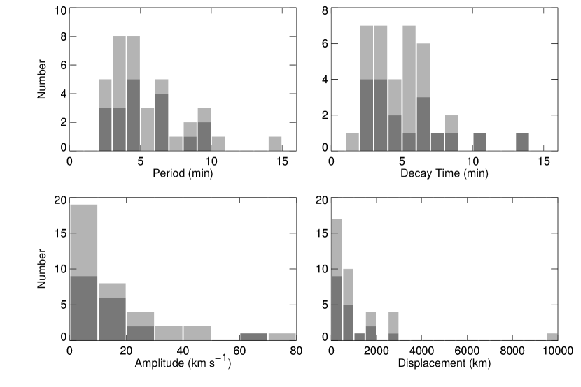
Figure 5.— Histograms showing the distributions of period, decay time, amplitude, and displacement measured from the BCS data. Each bar shows the total number of events in the bin with the dark gray showing the S XV contribution and the light gray showing the Ca XIX contribution.

4. BCS OSCILLATION MODES

The transverse loop oscillations observed with TRACE are thought to be fast kink mode MHD oscillations (Aschwanden et al., 2002). Those observed with SUMER have been interpreted as slow standing mode MHD waves (Wang et al., 2003b). Comparison of the averages in Table 2 with the TRACE and SUMER results suggests that the BCS values are closer to those from TRACE than those from SUMER. The overall picture, however, is not entirely clear. Because exposure times for the SUMER observations tended to be quite long ($>50$ s), those observations are not sensitive to the shortest periods observed with the BCS. On the other hand, as shown in Figure 2, the BCS data often only extend for 20 minutes or less. Thus, for many events, they would not be sensitive to the longer periods seen in the SUMER data. It might be speculated, though, that the slow Doppler shift evolution seen in the S XV data in Figure 2 and partially removed by the background polynomial fits to the data is actually a portion of a longer period damped oscillation that is superimposed on those being measured in this paper.

For a loop of length $L$, the period of a slow-mode wave is given by

$$P=\frac{2L}{jc_{T}}\,,$$ (4)

where $j$ is the node number, usually assumed to be 1, and $c_{T}$ is the slow magnetoacoustic speed, which is close to the sound speed (Roberts et al., 1984). Early in the time period where the BCS Doppler shift oscillations are observed, the temperatures measured in the S XV channel are around 12 MK, while those measured in the Ca XIX channel are around 14 MK (see, e.g., Figure 2). For a coronal composition plasma, the sound speed is given by $c_{s}\approx 0.152\sqrt{T}$ km s^-1. Thus, if the oscillations are slow standing mode waves, the average periods in the table and their standard deviations imply loop lengths of about $82\pm 35$ Mm for S XV and $99\pm 55$ Mm for Ca XIX—roughly 113 and 137 arcsec, respectively. For semicircular loops with the above lengths, this corresponds to loop radii of 26 and 32 Mm, respectively, or 36 and 44 arcsec.

The plasma observed with the BCS S XV and Ca XIX channels tends to have higher temperatures than those measured for the same events using the Yohkoh soft X-ray telescope (SXT) (e.g., Doschek, 1999). Thus, it is not clear that the the sizes of the loops observed with SXT are appropriate for comparison with the above estimates. Moreover, many of the flares are at the limb and have portions of the loop occulted by the solar disk.

There are, however, some interesting events. The 1992 July 17 flare was not occulted and clearly showed a loop-like structure. This flare was included in a study of occulted and nonocculted flares by Mariska & McTiernan (1999). The loop is near the limb, so projection effects make a length determination difficult. A. Winebarger (2005, private communication) has used the SXT Be filter data for this flare to examine possible geometries for the loop. The geometry is difficult to define, but if the aspect ratio is near one (a semicircular loop), the length would be approximately 60 Mm. The frequencies listed for this flare in Table 1 imply lengths of 47 and 61 Mm for the S XV and Ca XIX observations, respectively. Given the uncertainties in connecting the SXT images to the plasma being observed with the BCS S XV and Ca XIX channels, these numbers are in excellent agreement.

If the oscillations are slow standing mode waves, other observable physical quantities should also be oscillating. For a sound wave, $v=c_{s}\delta\rho/\rho$. Thus, for a 12 MK plasma, $\delta\rho/\rho\approx 0.04$, a very small density fluctuation. Even though the intensity is proportional to the square of the density, this is a small fluctuation. Also, since the BCS images the entire loop, it would be difficult to see this small an oscillation when the entire loop is observed since for the fundamental mode the density oscillation has anti-nodes at the two footpoints of the loop, and the oscillations at these two anti-nodes are in anti-phase. For the partially occulted flares, one might expect, however, to see intensity fluctuations.

The four panels of Figure 6 show the results of fitting a polynomial background and exponentially decaying sine wave to the intensity data for the 1991 October 21 flare. Only the data between the vertical dashed lines were fitted. The top panels show the intensity data and the best-fit background trend. In both BCS channels, the background was fit with a cubic polynomial. Error bars are not included in the plots. Since the integration times for the portion of the data used in the fits were generally 21 s, the errors for a count rate of 2500 counts s^-1 are about 11 counts s^-1. For a 1500 counts s^-1 count rate, the corresponding error is about 8 counts s^-1. Thus the fluctuations fitted in the bottom two panels are well above the level expected from counting statistics.

Table 3 summarizes the intensity fitting results for this flare. While the origin of the time values for the fitting calculation in each channel was tied to the time of the first fitted spectrum, the results in the table for the Ca XIX channel have been adjusted to correspond to the initial time used for the S XV fits. The beginning time for the S XV intensity fits is the same as the beginning time used for the velocity fits for this flare listed in Table 1. Thus the intensity results for the two channels can be directly compared with each other and with the results for the same flare shown in Table 1.

The periods and decay times of the intensity fluctuations are comparable with the characteristics of the fits to the Doppler shift measurements for this flare. The phases for the fits to the intensity measurements are, however, different. This is most easily visualized by comparing the times of the first peak in the fits to the Doppler shifts in Figure 3 with those of the fits to the intensity fits in Figure 6. For S XV, the intensity peak occurs 1.54 minutes after the Doppler shift peak. This corresponds to a delay of 1/4 of the period, strongly suggesting that the oscillations observed in this flare are due to slow standing-mode MHD waves (Sakurai et al., 2002).

Figure 6.— Averaged BCS S XV and Ca XIX intensity data and decaying sine wave fits for the 1991 October 21 flare. Only the data between the vertical dashed lines have been fitted. Time is measured from 02:47:34 UT—the same starting time used for Figure 3.

Additional evidence for intensity oscillations in the 1991 October 21 flare is provided by data from the GOES satellite. One-minute integration time data for this flare are available from the National Geophysical Data Center. Polynomial fits to the same time intervals used for the S XV intensity data for this flare reveal the same oscillations in the residual signal in both the 1–8 and 0.5–4 Å GOES channels.

One curious feature of the intensity fluctuations appears to be a tendency for the oscillation in the residual signal to be more obvious in the data from higher temperature plasma. Note, for example in Figure 6, that the oscillations in the Ca XIX intensity are better defined than those in the S XV residuals. This also appears to be the case for the two GOES channels. Examination of the the intensity data from the BCS Fe XXV channel also shows oscillations in the residual intensities for this flare that are well defined. This is probably due to the reduced amount of background emission at higher temperatures that must be removed from the oscillatory signal and suggests that oscillations should be detectable in the lower energy channels for occulted flares observed with the Hard X-Ray Telescope on Yohkoh and those observed with the Ramaty High Energy Solar Spectroscopic Imager.

Intensity fluctuations are not present in all the flares that exhibit Doppler shift oscillations. Thus it is worthwhile to ask whether some of the flares might be exhibiting fast kink mode oscillations which correspond to the displacement of an entire flux tube. For a loop of length $L$, the period of the wave is given by

$$P=\frac{2L}{jc_{k}}\,,$$ (5)

where $j$ is the node number, usually assumed to be 1, and $c_{k}$ is the kink speed (Roberts et al., 1984). For a flux tube with an internal magnetic field strength equal to the external field strength, but a much greater plasma density, $c_{k}\approx\sqrt{2}c_{A}$, where $c_{A}$ is the Alfvén speed.

For the 1992 Jul 17 event discussed above, the estimated loop length of 60 Mm and a period of 3.3 min (the average of the S XV channel and Ca XIX channel results for this event) result in an Alfvén speed of about 600 km s^-1. Electron densities from 10¹⁰ to 10¹² cm^-3 then imply magnetic field strengths ranging from 27 to 275 G. For a number of flares observed with the Naval Research Laboratory S082A spectrograph on Skylab, Keenan et al. (1998) used density sensitive emission lines of Ca XVI to determine an average electron density of $2.9\times 10^{11}$ cm^-3. This value would imply a magnetic field strength of about 128 G. The low end of this range of field strengths is consistent with ranges that are typically quoted for flaring loops (e.g., Tsuneta, 1996).

Taking a temperature of 14 MK, a density of $3\times 10^{11}$ cm^-3, and magnetic field strength of 128 G results in a plasma $\beta$ of about 1.8. For a density of $10^{10}$ cm^-3 and a field strength of 27 G, the plasma $\beta$ is about 1.3. The same conclusion was reached by Wang et al. (2002), who obtained values near two for $\beta$. Generally, the coronal plasma is thought to be low beta plasma. Moreover, equation (5) has been derived by assuming that the plasma is low-$\beta$. Thus further analysis of the possibility that some of the observed Doppler shift oscillations are due to kink modes will require a more careful examination of the governing equations. The existence of intensity fluctuations shifted by $1/4$ phase in some of the flares argues strongly that all of the flare Doppler shift oscillations observed with BCS are slow mode standing waves.

5. DAMPING OF THE OSCILLATIONS

Linear slow wave dissipation theory predicts that the decay time for an oscillation should scale as $P^{2}$, where $P$ is the oscillation period (Porter et al., 1994). More detailed calculations predict different slopes. Ofman & Wang (2002) have investigated the damping of the slow-mode oscillations observed with SUMER using one-dimensional hydrodynamic simulations. They considered both damping by thermal conduction and compressive viscosity and found that for the SUMER observations the damping was dominated by thermal conduction. For the conditions in the loops observed with SUMER, they found that the scaling goes as $P^{1.17}$ for a loop temperature of 6.3 MK and as $P^{1.07}$ for a loop temperature of 6.8 MK. Ofman & Wang (2002) attributed the smaller slope to the nonlinearity of the observed oscillations; they assumed $A_{0}/c_{s}=0.18$.

Figure 7 shows the decay time of the oscillations plotted against the period for all the events observed with the BCS. The line in the plot is the best fit to all the data and corresponds to $t_{\textrm{decay}}=2.30P^{0.39}$—a much smaller slope than that determined by Wang et al. (2003a) from the SUMER observations. The BCS results, however, apply to a much higher temperature plasma, 12 to 14 MK, than the SUMER observations. (While the peak in the S XV emissivity function is at about 6.8 MK, the spectral fitting to the observations, which include temperature-sensitive lines, results in the higher temperature.) For the SUMER data, the highest temperature emission line in which oscillations were typically observed was from Fe XXI with a formation temperature of about 7.0 MK. The Ofman & Wang (2002) calculations show that the slope decreases for increasing plasma temperature. Since the damping is by conduction, which scales as $T^{2.5}$, one might expect a sizable change in the slope as the loop temperature increases. On the other hand, the oscillations observed with the BCS have a much smaller amplitude. For a temperature of 12 to 14 MK, the average amplitude of 17.1 km s^-1 leads to $A_{0}/c_{s}\approx 0.04$, somewhat less nonlinear than is the case for the SUMER oscillations. Moreover, there is clearly considerable uncertainty in the BCS results, especially in the decay time determination.

Figure 7.— The measured decay time vs. period for the events observed with the BCS. Error bars ($1\sigma$) for both the period measurement and the decay time measurement are shown. The solid line shows the best fit relationship between the log of the period and the log of the decay time.

While the Ofman & Wang (2002) calculations suggest that comparisons between the BCS and SUMER observations may be hindered by the different formation temperatures of the emission lines being observed, it is useful to plot all the data together, especially since the BCS observations explore shorter periods than are available with the SUMER data. Figure 8 shows the decay time vs. period for the BCS events plotted in Figure 7 along with the results for events observed with SUMER and TRACE. For the SUMER data, only the 49 cases fitted by Wang et al. (2003a) have been included. Note that while the TRACE data points lie in the same period interval on the figure as the BCS data, they generally have longer decay times than the BCS data—further suggesting that the TRACE data represent a different kind of oscillation. Of course, the loops measured in the TRACE observations contain plasma at significantly lower temperatures, $\sim 1$ MK, than those observed with the BCS and SUMER.

Figure 8.— The measured decay time vs. period for the events observed with the BCS, the SUMER events reported by Wang et al. (2003a), and the TRACE events reported by Ofman & Aschwanden (2002), Wang & Solanki (2004), and Verwichte et al. (2004). The dashed line shows the best fit relationship between the log of the period and the log of the decay time plotted in Figure 7, the dot-dash line shows a fit to the Wang et al. (2003a) data, and the solid line shows the fit to the combined BCS and SUMER data sets.

Also plotted on the figure are the least squares fits to the BCS data that are shown on Figure 7, the SUMER data, and the combined BCS and SUMER data. The fit to the combined BCS and SUMER data results corresponds to the expression $t_{\textrm{decay}}=1.30P^{0.81}$.

6. DISCUSSION

It is generally assumed that the emission observed with the BCS is produced in the loop or loops that have been heated by the flare energy release process. Thus the observed oscillations are probably triggered by the heating due to the flare energy release. The observation of damped slow-mode oscillations in the high-temperature flare plasma then presents interesting challenges for some of the current models for the evolution of flaring loops. TRACE observations clearly show that in the decay phase solar flares exhibit many loop-like structures (e.g., Warren et al., 1999; Warren, 2000; Aschwanden & Alexander, 2001). This has led to attempts to model a flare as a succession of independently heated threads (Warren & Doschek, 2005; Warren, 2005). To model a GOES M2.0 flare, Warren (2005) needed 50 individual threads, with each one introduced 50 s after the previous thread. Each thread was heated using a triangular heating function with a width of 200 s.

The model fits the BCS S XV and Ca XIX channels well, yet over the roughly 5–10 minute period where one sees oscillations in most of the events discussed here, many individual threads contribute to the signal observed in the BCS channels. This would seem to suggest that either multiple threads contain damped slow-mode waves with the same parameters, or that an individual thread is dominating the emission observed over the time interval where the oscillations are observed. The model described in Warren (2005) is still under development, so it is not clear, for example, what the time dependent Doppler shifts look like when the ensemble of threads is considered in their entirety as might be the case for a flare observed on the disk, or when only the top portions of the threads are considered as might be the case for a flare that is partially occulted by the solar limb. It is also not yet clear what the minimum number of threads is that will still smoothly reproduce the light curves observed with the instruments with which the data have been compared.

Yohkoh observed the flares that triggered a number of the events analyzed by Aschwanden et al. (2002). Only the 1999 October 25 flare exhibited oscillations in the BCS data that could be fit using equation (1). The three features observed with TRACE exhibited oscillation periods that ranged from 2.38 to 2.70 minutes, with one feature showing a decay time of 3.33 minutes. In contrast, the BCS S XV and Ca XIX observations show periods of 9.7 and 9.1 minutes and decay times of 10.0 and 5.68 minutes, respectively. Thus, while the oscillations may be triggered by the same event, it is unlikely that TRACE and the BCS are observing the same oscillations. This is not surprising given the significant differences in temperature sensitivity between the BCS and TRACE.

Yohkoh SXT data are available for 18 of the 20 flares included in Table 1. Most of the flares are at the limb and very little looplike structure can be discerned in the data. Ten of the flares are included in the Sato et al. (1993) catalog of flares observed with the Yohkoh SXT and Hard X-Ray Telescope (HXT). The images in the catalog made from the HXT data generally show only one emitting feature—again making it difficult to determine loop size parameters. In none of the flares have I been able to determine whether the oscillations are taking place in a pre-existing loop or the flaring loop itself. Some of the SXT data sets, however, provide extensive, high-cadence observations of the event. Studies of the time histories of the intensities in the individual pixels may provide additional insight into the nature of the oscillations. This will be the topic of a future investigation.

Of the 103 flares observed by the Yohkoh BCS for this study, only the 20 in Table 1 exhibited Doppler-shift oscillations that could be easily fit with a well-defined decaying sine wave. As I mentioned earlier, an additional 18 events could be fitted, but were not used. Many of the other events, though, did exhibit significant Doppler-shift fluctuations. Since the BCS observes all the flaring plasma at the temperature of formation of the S XV and Ca XIX lines, this is probably an indication that multiple structures are exhibiting Doppler shift fluctuations that are out of phase. While no attempt was made to observe flares at all center-to-limb positions on the disk, the results in Table 1 clearly suggest the flares near the limb tend to show well-defined oscillations more frequently than those closer to disk center. Since the Yohkoh BCS observes the entire Sun, this may simply imply that flares for which a portion of the flaring loops are occulted by the solar limb provide a cleaner Doppler-shift signal.

Fitting the intensity fluctuations using equation (1) is more difficult than fitting the Doppler-shift fluctuations. While the background trend in the Doppler shift data can usually be removed with just one or two terms in equation (2), the underlying trend in the intensities usually requires more terms. If one tries to detrend the intensity data with the peak in the intensity included, the background removal is even more complex. Moreover, including the background terms as adjustable fitting parameters often results in the fit selecting a damped sine wave with a substantial amplitude, up to 25% of the peak intensity, with a significantly altered background light curve, which is probably not a true representation of the oscillation.

While I will defer a detailed analysis of the intensity fluctuations to a future paper, a preliminary examination of the S XV intensity fluctuations for the 17 flares in Table 1 for which S XV Doppler-shift fits were available was conducted. All 17 flares could be fitted with expressions of the form of equation (1). Of those 17, only six showed phase lags that were judged to be consistent with that expected for a slow standing-mode MHD wave. Fits to five of the remaining flares resulted solutions that were viewed as having unrealistic background terms. Fits for the remaining six flares looked reasonable, but the phases were not close to the expected 1/4 period lag. Five of the six flares with reasonable phase lags were at the limb. The flares at the limb generally show only a small concentrated emitting region in the SXT data.

Detection of damped intensity fluctuations for some flares in the S XV, Ca XIX, and Fe XXV wavelength bands and in broad-band GOES observations raises the intriguing possibility that spatially-resolved coronal loop observations with sufficient signal-to-noise and short enough exposure times may provide a wealth of information on the standing slow-mode waves. It may be possible to detect damped intensity oscillations in the Yohkoh SXT data. McKenzie & Mullan (1997) have searched for oscillations in SXT image sequences, finding some evidence for relatively short period fluctuations, 9.6 to 61.6 s. Their time-series analysis may, however, have missed the kinds of intensity fluctuations reported here. The high sensitivity and spatial resolution Soft X-Ray Telescope and EUV Imaging Spectrometer instruments on the upcoming Solar-B satellite scheduled for launch in 2005 August should prove ideal for this kind of observation.

Table 1Doppler Shift Oscillation Properties

				$A_{0}$	$\omega$	$\phi$	$\lambda$
$t_{0}$ (UT)		Class	Location	(km s-1)	(rad min-1)	(rad)	(min-1)
1991 Oct 7	10:16:57	C9.9	S13W82	$66.18\pm 5.91$	$1.36\pm 0.04$	$-5.80\pm 0.07$	$0.273\pm 0.047$
				$38.92\pm 11.54$	$1.27\pm 0.10$	$-5.63\pm 0.06$	$0.653\pm 0.138$
1991 Oct 21	02:47:34	C4.3	S06E89y	$18.89\pm 1.04$	$0.99\pm 0.04$	$-5.35\pm 0.17$	$0.276\pm 0.020$
				$10.82\pm 2.22$	$1.17\pm 0.12$	$-5.54\pm 0.17$	$0.497\pm 0.131$
1992 Jan 15	08:59:21	C5.0	S18W90	$6.93\pm 0.76$	$1.39\pm 0.09$	$-5.54\pm 0.17$	$0.388\pm 0.086$
				$9.69\pm 2.10$	$1.10\pm 0.08$	$-4.98\pm 0.30$	$0.253\pm 0.068$
1992 Feb 26	01:35:57	M1.3	S15W90	$22.63\pm 2.74$	$2.47\pm 0.11$	$-5.82\pm 0.21$	$0.498\pm 0.056$
				$20.40\pm 6.11$	$1.93\pm 0.10$	$-4.00\pm 0.27$	$0.298\pm 0.115$
1992 Mar 16	06:06:15	C5.8	S25W21	$9.09\pm 0.28$	$1.32\pm 0.05$	$-0.84\pm 0.04$	$0.404\pm 0.028$
				$7.93\pm 2.17$	$1.44\pm 0.07$	$-0.24\pm 0.20$	$0.160\pm 0.110$
1992 Apr 19	02:11:32	C3.9	N15E78	$6.49\pm 1.74$	$2.16\pm 0.05$	$-0.50\pm 0.20$	$0.117\pm 0.063$
				$4.38\pm 2.96$	$1.58\pm 0.23$	$-5.17\pm 0.59$	$0.193\pm 0.285$
1992 Apr 20	06:33:25	C3.6	S15E39	$5.89\pm 1.05$	$1.94\pm 0.05$	$-4.69\pm 0.21$	$0.149\pm 0.043$
				$\cdots$	$\cdots$	$\cdots$	$\cdots$
1992 May 27	14:37:53	C7.1	N23W59	$11.01\pm 2.05$	$2.48\pm 0.06$	$-3.58\pm 0.13$	$0.391\pm 0.090$
				$6.00\pm 1.84$	$2.22\pm 0.07$	$-2.30\pm 0.26$	$0.117\pm 0.075$
1992 Jul 4	22:49:16	C6.9	S12E89	$6.22\pm 1.93$	$0.67\pm 0.06$	$-2.94\pm 0.13$	$0.229\pm 0.078$
				$6.45\pm 1.10$	$0.58\pm 0.08$	$-2.74\pm 0.22$	$0.181\pm 0.098$
1992 Jul 17	22:36:31	C5.3	S11W87	$4.49\pm 1.23$	$2.09\pm 0.05$	$-2.62\pm 0.17$	$0.214\pm 0.079$
				$7.87\pm 4.82$	$1.76\pm 0.11$	$-1.16\pm 0.52$	$0.202\pm 0.139$
1992 Aug 24	01:12:48	C2.2	N14W90	$\cdots$	$\cdots$	$\cdots$	$\cdots$
				$7.58\pm 2.94$	$2.99\pm 0.25$	$-2.90\pm 0.40$	$0.474\pm 0.217$
1992 Oct 12	21:50:44	C2.5	S16W88	$11.37\pm 1.87$	$1.60\pm 0.06$	$-2.43\pm 0.05$	$0.284\pm 0.090$
				$8.77\pm 2.79$	$1.76\pm 0.17$	$-2.86\pm 0.41$	$0.235\pm 0.130$
1992 Oct 27	22:14:55	C5.4	N08W90	$14.03\pm 1.44$	$0.96\pm 0.04$	$-1.07\pm 0.20$	$0.165\pm 0.028$
				$16.96\pm 3.94$	$1.25\pm 0.14$	$-2.18\pm 0.46$	$0.156\pm 0.107$
1992 Nov 5	06:24:08	M2.0	S17W88	$9.22\pm 0.60$	$0.92\pm 0.02$	$-4.37\pm 0.11$	$0.072\pm 0.017$
				$24.41\pm 2.00$	$0.74\pm 0.02$	$-2.90\pm 0.10$	$0.159\pm 0.018$
1993 Feb 1	10:07:38	C6.9	S11E90	$3.65\pm 0.32$	$1.55\pm 0.23$	$-1.94\pm 0.54$	$0.270\pm 0.058$
				$3.52\pm 1.66$	$1.69\pm 0.26$	$-1.64\pm 0.55$	$0.253\pm 0.219$
1993 Apr 15	09:08:36	C1.2	S19W90y	$26.00\pm 1.52$	$0.78\pm 0.01$	$-1.60\pm 0.05$	$0.142\pm 0.009$
				$42.19\pm 4.08$	$0.83\pm 0.03$	$-2.04\pm 0.14$	$0.193\pm 0.016$
1993 Sep 26	10:22:47	C3.4	N12E90	$15.43\pm 4.23$	$0.96\pm 0.03$	$-3.69\pm 0.25$	$0.173\pm 0.030$
				$76.32\pm 17.88$	$0.42\pm 0.03$	$-0.68\pm 0.04$	$0.193\pm 0.053$
1994 Feb 27	09:11:09	M2.8	N08W88	$3.60\pm 0.60$	$1.39\pm 0.03$	$-0.55\pm 0.04$	$0.143\pm 0.031$
				$4.75\pm 1.16$	$1.40\pm 0.04$	$-0.67\pm 0.19$	$0.190\pm 0.055$
1999 Oct 25	06:36:18	M1.7	S18E88y	$17.25\pm 1.52$	$0.65\pm 0.02$	$-0.10\pm 0.09$	$0.100\pm 0.017$
				$33.17\pm 4.29$	$0.69\pm 0.02$	$-0.35\pm 0.06$	$0.178\pm 0.037$
2000 Jul 14	00:41:45	M1.5	N20W80y	$\cdots$	$\cdots$	$\cdots$	$\cdots$
				$43.01\pm 7.50$	$0.96\pm 0.04$	$-5.88\pm 0.12$	$0.341\pm 0.057$

Table 2Average Doppler Shift Oscillation Properties

Parameter	S XV	Ca XIX	Combined	TRACE	SUMER
Oscillation Period (min)	$5.2\pm 2.2$	$5.8\pm 3.2$	$5.5\pm 2.7$	$5.4\pm 2.3$	$17.6\pm 5.4$
Decay Time (min)	$5.5\pm 3.1$	$4.7\pm 1.8$	$5.0\pm 2.5$	$9.7\pm 6.4$	$14.6\pm 7.0$
Amplitude (km s-1)	$14.4\pm 14.5$	$19.6\pm 19.2$	$17.1\pm 17.0$	$42\pm 53$	$98\pm 75$
Displacement (km)	$730\pm 742$	$1400\pm 2260$	$1070\pm 1710$	$2200\pm 2800$	$12500\pm 9900$
Decay Time to Period Ratio	$1.13\pm 0.65$	$0.98\pm 0.62$	$1.05\pm 0.63$	$1.8$	$0.85\pm 0.35$

Table 3Intensity Fitting Results

Parameter	S XV	Ca XIX
$A_{0}$ (counts s-1)	$41.5\pm 8.0$	$38.8\pm 7.1$
$\omega$ (rad min-1)	$1.05\pm 0.04$	$0.81\pm 0.04$
$\phi$ (rad)	$-0.72\pm 0.25$	$0.53\pm 0.25$
$\lambda$ (min-1)	$0.12\pm 0.04$	$0.14\pm 0.02$

References

- Arnaud & Rothenflug (1985) Arnaud, M., & Rothenflug, R. 1985, A&AS, 60, 425
- Aschwanden (2003) Aschwanden, M. J. 2003, in NATO Science Series : II: Mathematics, Physics and Chemistry, Vol. 124, Turbulence, Waves and Instabilities in the Solar Plasma, ed. R. Erdelyi, K. Petrovay, B. Roberts, & M. J. Aschwanden (Kluwer Academic Publishers, Dordrecht), 215–237
- Aschwanden & Alexander (2001) Aschwanden, M. J., & Alexander, D. 2001, Sol. Phys., 204, 91
- Aschwanden et al. (2002) Aschwanden, M. J., De Pontieu, B., Schrijver, C. J., & Title, A. M. 2002, Sol. Phys., 206, 99
- Aschwanden et al. (1999) Aschwanden, M. J., Fletcher, L., Schrijver, C. J., & Alexander, D. 1999, ApJ, 520, 880
- Bely-Dubau et al. (1982a) Bely-Dubau, et al. 1982a, MNRAS, 201, 1155
- Bely-Dubau et al. (1982b) Bely-Dubau, F., Faucher, P., Dubau, J., & Gabriel, A. H. 1982b, MNRAS, 198, 239
- Bevington (1969) Bevington, P. R. 1969, Data reduction and error analysis for the physical sciences (New York: McGraw-Hill)
- Culhane et al. (1991) Culhane, et al. 1991, Sol. Phys., 136, 89
- Doschek (1999) Doschek, G. A. 1999, ApJ, 527, 426
- Keenan et al. (1998) Keenan, F. P., Pinfield, D. J., Woods, V. J., Reid, R. H. G., Conlon, E. S., Pradhan, A. K., Zhang, H. L., & Widing, K. G. 1998, ApJ, 503, 953
- Kliem et al. (2002) Kliem, B., Dammasch, I. E., Curdt, W., & Wilhelm, K. 2002, ApJ, 568, L61
- Mariska (2005) Mariska, J. T. 2005, ApJ, 620, L67
- Mariska & McTiernan (1999) Mariska, J. T., & McTiernan, J. M. 1999, ApJ, 514, 484
- McKenzie & Mullan (1997) McKenzie, D. E., & Mullan, D. J. 1997, Sol. Phys., 176, 127
- Nakariakov et al. (1999) Nakariakov, V. M., Ofman, L., Deluca, E. E., Roberts, B., & Davila, J. M. 1999, Science, 285, 862
- Ofman (2002) Ofman, L. 2002, ApJ, 568, L135
- Ofman & Aschwanden (2002) Ofman, L., & Aschwanden, M. J. 2002, ApJ, 576, L153
- Ofman & Wang (2002) Ofman, L., & Wang, T. 2002, ApJ, 580, L85
- Porter et al. (1994) Porter, L. J., Klimchuk, J. A., & Sturrock, P. A. 1994, ApJ, 435, 482
- Roberts (2000) Roberts, B. 2000, Sol. Phys., 193, 139
- Roberts et al. (1983) Roberts, B., Edwin, P. M., & Benz, A. O. 1983, Nature, 305, 688
- Roberts et al. (1984) —. 1984, ApJ, 279, 857
- Roberts & Nakariakov (2003) Roberts, B., & Nakariakov, V. M. 2003, in NATO Science Series : II: Mathematics, Physics and Chemistry, Vol. 124, Turbulence, Waves and Instabilities in the Solar Plasma, ed. R. Erdelyi, K. Petrovay, B. Roberts, & M. J. Aschwanden (Kluwer Academic Publishers, Dordrecht), 167–192
- Sakurai et al. (2002) Sakurai, T., Ichimoto, K., Raju, K. P., & Singh, J. 2002, Sol. Phys., 209, 265
- Sato et al. (1993) Sato, J., Sawa, M., Yoshimura, K., Masuda, S., & Kosugi, T. 1993, The Yohkoh HXT/SXT Flare Catlogue, Tech. rep., Montana State University and The Institute for Space and Astronautical Science
- Schrijver et al. (2002) Schrijver, C. J., Aschwanden, M. J., & Title, A. M. 2002, Sol. Phys., 206, 69
- Schrijver & Brown (2000) Schrijver, C. J., & Brown, D. S. 2000, ApJ, 537, L69
- Tsuneta (1996) Tsuneta, S. 1996, ApJ, 456, 840
- Vainshtein & Safronova (1978) Vainshtein, L. A., & Safronova, U. I. 1978, Atomic Data and Nuclear Data Tables, 21, 49
- Vainshtein & Safronova (1985) —. 1985, Physica Scripta, 31, 519
- Verwichte et al. (2004) Verwichte, E., Nakariakov, V. M., Ofman, L., & Deluca, E. E. 2004, Sol. Phys., 223, 77
- Wang et al. (2002) Wang, T., Solanki, S. K., Curdt, W., Innes, D. E., & Dammasch, I. E. 2002, ApJ, 574, L101
- Wang & Solanki (2004) Wang, T. J., & Solanki, S. K. 2004, A&A, 421, L33
- Wang et al. (2003a) Wang, T. J., Solanki, S. K., Curdt, W., Innes, D. E., Dammasch, I. E., & Kliem, B. 2003a, A&A, 406, 1105
- Wang et al. (2005) Wang, T. J., Solanki, S. K., Innes, D. E., & Curdt, W. 2005, A&A, 435, 753
- Wang et al. (2003b) Wang, T. J., Solanki, S. K., Innes, D. E., Curdt, W., & Marsch, E. 2003b, A&A, 402, L17
- Warren (2000) Warren, H. P. 2000, ApJ, 536, L105
- Warren (2005) —. 2005, ApJ, submitted
- Warren et al. (1999) Warren, H. P., Bookbinder, J. A., Forbes, T. G., Golub, L., Hudson, H. S., Reeves, K., & Warshall, A. 1999, ApJ, 527, L121
- Warren & Doschek (2005) Warren, H. P., & Doschek, G. A. 2005, ApJ, 618, L157