The impact on the general properties of HII galaxies in the local universe of the visibility of the [OIII]$\lambda 4363$ line.

Abstract

We present a statistical study of a very large sample of HII galaxies taken from the literature. We focus on the differences in several properties between galaxies that show the auroral line [OIII]$\lambda 4363$ and those that do not present this feature in their spectra. It turns out that objects without this auroral line are more luminous, more metal-rich and present a lower ionization degree. The underlying population is found to be much more important for objects without the [OIII]$\lambda 4363$ line, and the effective temperature of the ionizing star clusters of galaxies not showing the auroral line is probably lower. We also study the subsample of HII galaxies whose properties most closely resemble the properties of the intermediate-redshift population of Luminous Compact Blue Galaxies (LCBGs). The objects from this subsample are more similar to the objects not showing the [OIII]$\lambda 4363$ line. It might therefore be expected that the intermediate-redshift population of LCBGs is powered by very massive, yet somewhat aged star clusters. The oxygen abundance of LCBGs would be greater than the average oxygen abundance of local HII galaxies.

1 Introduction

The term “HII galaxy” currently denotes dwarf emission line galaxies undergoing violent star formation (VSF)(Melnick, Terlevich, & Moles, 1985), a process by which thousands of massive stars (m$\geq$20 M_⊙) have recently been formed in a very small volume (a few parsec in diameter) and on the timescale of only a few million years. HII galaxies comprise a subset of the larger class of objects referred to as “blue compact galaxies” (BCG). At optical wavelengths, the observable properties of HII galaxies are dominated by the young component of their stellar population and their spectra are essentially identical to those of Giant Extragalactic HII Regions (GEHR) in nearby spiral and irregular galaxies. The analysis of these spectra shows that many HII galaxies are metal poor objects, some of them – IZw18, UGC4483 – being the most metal poor systems known.

Although it was initially thought that HII galaxies are compact, essentially spheroidal, in fact they show a variety of morphologies with an appreciable number of them having two or more components and showing clear signs of interactions (Telles et al., 1997). Actually, IIZw40, one of the first HII galaxies identified, when imaged at sufficiently high resolution looks like the result of a merger of two separate subsystems (Melnick et al. (1992)).

The study of blue, compact star forming systems in the distant universe is an important ingredient in galaxy formation and evolution theories. Although such systems probably were not much more powerful than many local HII galaxies, it is believed that they were much more common in the past than they are today and therefore they harboured a great amount of the star formation density in the universe. This fact makes of high redshift blue compact galaxies very interesting targets for observation. Unfortunately, since they are located at large distances, their study can only be carried out with a combination of Hubble Space Telescope providing high spatial resolution and 10-m class telescopes providing high collecting power. Nevertheless, data on this kind of objects are accumulating fast.

Luminous Compact Blue Galaxies (LCBG) are defined as very luminous (M_B $\leq$ -17.5), compact ($\mu_{B}\leq 21.5$mag arcsec^-2) and blue (B-V) $\leq$ 0.6) galaxies undergoing a major burst of star formation (Hoyos et al. 2004). According to this definition LCBG, as a family, include the most luminous local HII galaxies. In principle, since they belong to the general category of emission line objects, the techniques used for their analysis are those already developed for the same class of objects in the local universe. However, in order to interpret these analyses properly in terms of evolution, a good comparison sample needs to be available.

There have been many studies of HII galaxies in the local universe, and the errors and uncertainities in the determination of their properties are supposed to be well understood. However, due to the importance of the metallicity effects in controlling the gaseous emission line spectra, most of these studies have been restricted to a subsample that allows a good direct determination of their chemical abundances, through the detection and measure of the weak [OIII] $\lambda$ 4363 Å line. This implies the selection of the highest excitation objects which, in principle, can’t be considered to be a good comparison sample.

The purpose of the present work is to analyse a large sample of local universe HII galaxies. In particular two issues are addressed. The first one is the comparison of several observational parameter distributions for objects with and without measurements of the [OIII]$\lambda 4363$ Å emission line and the statistical analysis of the whole HII galaxy sample to define their average properties. The second one is the statistical study of a subsample consisting of the most luminous objects, local representatives of LCBG, and its comparison to the whole HII galaxy sample.

The cosmology assumed through this paper is a flat universe with H₀=70km s^-1 Mpc^-1.

2 The sample selection.

We have compiled published emission line measurements of local HII galaxies from different sources. The data gathered, together with the works we have used to compile the galaxy sample are given in table 1. The vast majority of the objects selected for this study were discovered using Schmidt telescopes, searching for strong emission lines or blue colors. Sources with strong emission lines are easiliy detected through objective prism surveys. This technique is best suited to detect objects with high equivalent widths and line strengths. Objects with strong continua are lost in these surveys, since the emission lines are swallowed by the continuum. On the other hand, galaxies with weak lines which have evolved past their peaks of star formation but which are still quite blue are found through colour selection techniques.

The objects from references 6 and 10 come from the Tololo (Smith, Aguirre, & Zemelman, 1976) and University of Michigan (UM) (MacAlpine, Lewis, & Smith, 1977) objective prism surveys. The limiting magnitude is about 19.0. The spectroscopic observations for these samples were taken using several telescopes and detectors, and the observing conditions were not always good. Some of the observations were carried out at Las Campanas 2.5m telescope, using narrow apertures. These observations therefore can’t provide absolute fluxes. They were also affected by second order contamination. The rest of the spectra were obtained using the 3.6m at ESO. The slit aperture was 8″, and the spectrophotometry is accurate to 10%.

The objects from reference 7 are the brightest galaxies from the Calan-Tololo objective prism survey (Maza et al., 1989). Its limitinig magnitude is 17.5. The spectra were obtained using a variety of detectors (Vidicon, 2DF, CCDs), and the apertures used range from 2″to 4″. The spectra were flux calibrated.

The HII galaxies from reference 19 are located in the voids of the digitized Hamburg Quasar Survey (Hagen et al., 1995). The limiting magnitude of the objective prism survey is 18.5. The data presented in this work were gathered using the 2.2m telescope at the German-Spanish observatory at Calar Alto, Spain, under good photometric conditions using a 4″slit. This is enough to encompass most of the line-emitting region.

The objects from the reference 15 were selected from the Case survey (Pesch & Sanduleak, 1983). This survey searches simultaneously for both a UV excess and strong emission lines. The limiting magnitude is 16.0. The data for this spectroscopic follow-up study were obtained on 9 observing runs, using different telescopes and detectors. The majority of the objects in this sample were observed using CCD detectors, and the spectra were flux calibrated. The slit widths used were 2.4″and 3.0″. The spatial region extracted spanned all of the line emission, but did not cover all of the continuum emission.

The objects from the references 13, 14, 16, 17 and 18 were taken from the first Byurakan Survey (FBS, also known as the Markarian survey,(Markarian, 1967)) and the second Byurakan Survey (SBS)(Markarian, Lipovetskii, & Stepanian, 1983). The FBS is another objective prism survey that searches for galaxies with a UV excess, and its limiting photographic magnitude is 15.5. Selection of the SBS objects was done according to the presence of strong UV continuum and emission lines. The SBS was carried out using the same Schmidt telescope as the FBS, and its limiting photographic magnitude is 19.5. The observations presented in 13, 14, 16 and 17 are high S/N spectra, taken with the Ritchey-Chretien spectrograph at the Kitt Peak National Observatory (KPNO) 4m telescope, with the T2KB CCD. The slit width used was 2″, and the nights were transparent. The spectroscopic observations from reference 18 were done using the Ritchey-Chretien spectrograph at the KPNO 4m telescope, and with the GoldCam spectrograph at the 2.1 m KPNO telescope. In the majority of cases, a 2″slit was used.

Initially, we compiled objects with data on, at least, the intensities of the following emission lines: [OII] $\lambda\lambda$ 3727,29 Å , [OIII] $\lambda$ 4363 Å , [OIII] $\lambda\lambda$ 4959, 5007 Å , and [SII] $\lambda\lambda$ 6717, 6731 Å . The hydrogen Balmer recombination lines were also required in order to allow a proper reddening correction. The emission lines of [SII] allow the determination of the electron density (see e.g. Osterbrock 1989) and can also be used, as well as the lines of [OII], to estimate the ionization parameter of the emitting gas. The intensities of the auroral and nebular [OIII] emission lines are needed in order to derive accurate values of the electron temperature, and hence of the oxygen abundance. Objects meeting these requirements belong mostly to references 6, 10, 13, 14 and 16. For all the objects in these samples, data on the intensity and equivalent width of H$\beta$ are provided. We have also included data from references 7 and 2, although they lack data on the H$\beta$ equivalent width and line intensity respectively.

Our initial sample was later enlarged to include objects with the same information as above but with no data on the [SII] lines, for which a low density regime was assumed. This is probably not a bad assumption since the average electron density derived for the galaxies with [SII] data is around 200 cm^-3.

Finally, a third enlargement was made to include objects with no reported measurements of the [OIII] $\lambda$ 4363 Å line. These may correspond to objects with low surface brightness and/or low excitation and are generally excluded from emission-line analyses of samples of HII galaxies since the derivation of their oxygen abundances require the use of empirical calibrations which are rather uncertain (see e.g. Skillman 1989). These objects represent, however, a large fraction of the observed HII galaxies. Most of them have been taken from references 6, 19 and 15. The latter reference does not provide absolute intensities for the hydrogen recombination lines.

The final sample comprises 450 objects: 236 with data on the [OIII] $\lambda$ 4363 Å line and 214 with no observations of this line. These data have been obtained according to different selection criteria and using different instruments and techniques, and the parent populations of the different samples used are different. The presented sample can’t be considered as complete in any sense. In particular, line selected samples of galaxies are complete to a given line+continuum flux, whereas color selected samples will be complete to a given apparent magnitude. The galaxy sample presented here constitutes, however, the largest sample of local HII galaxies with good quality spectroscopic data, to our knowledge. However, the sample is very inhomogenous, due to different instrumental setups, observing conditions and reduction procedures. An accuracy analysis is therefore needed. This was done by comparing the observations for a few very well studied objects – e.g. IZw18, IIZw40, Mk36 – for which several independent observations exist. We have treated them as individual data in order to examine the external observational errors. The average error in redshift determinations is 5%. The average error in H$\beta$ fluxes is 45%, and the average error in the equivalent width of H$\beta$, W_β is 16%. Bin widths in the forthcoming histograms were chosen to be wide enough to engulf these errors. It is also important to note that, however large these numbers seem to be, they were derived from the nearest, brightest and best studied objects. These sources are sensitive to the full range of the aforementioned uncertainities, and are particularly affected by aperture issues (several components, different position angles for the slit, etc). More distant objects will be less affected by such effects, and their measurements will probably be more accurate. The errors previously presented are likely to be upper limits to the real uncertainities.

Table 1 lists the emission line properties of the sample objects. Column 1 gives the name of the object as it appears in the reference indicated in column 2. Column 3 gives the galaxy redshift (cz). Columns 4 to 9 give the reddening corrected emission line intensities, relative to that of H$\beta$, of: [OII] $\lambda\lambda$ 3727,29 Å, [OIII] $\lambda$ 4363 Å, [OIII] $\lambda$ 4959 Å, [OIII] $\lambda$ 5007 Å, [SII] $\lambda$ 6717 Å and [SII] $\lambda$ 6731 Å. Column 10 gives the value of the logarithmic extinction at H$\beta$, c(H$\beta$). Column 11 gives the reddening corrected H$\beta$ flux, in ergs cm^-2 s^-1. Finally, columns 12 and 13 give the equivalent width of the H$\beta$ and [OIII] $\lambda$ 5007 Å lines in Å. Only an example of the table entries are shown, the complete table being available in the online version of the paper.

Table 1: Partial list of galaxies included in this study.

Object.	Reference.	cz	$\lambda 3727$	$\lambda 4363$	$\lambda 4959$	$\lambda 5007$	$\lambda 6584$	$\lambda 6716$	$\lambda 6731$	c(H$\beta$)	$\log\mathrm{F(H}\beta\mathrm{).}$	$W_{\beta}$	$W_{\lambda 5007}$
UM439	6	1199	0.846	0.125	2.611	7.732	0.037	0.093	0.061	0.00	-13.44	160	1325
UM448	6	5396	2.736	0.034	0.961	2.826	0.392	0.277	0.197	0.27	-12.98	43	127
UM448	17	5498	2.776	0.030	0.867	2.599	0.409	0.366	0.285	0.33	-12.60	49	…
UM461	6	899	0.455	0.157	2.136	6.434	0.020	0.040	0.032	0.00	-13.20	342	2254
UM461	17	1007	0.527	0.136	2.039	6.022	0.021	0.052	0.042	0.12	-13.47	223	…
UM463	10	1199	1.255	0.153	1.942	5.687	0.078	0.088	0.091	0.05	-13.77	127	716
UM462SW	6	899	1.599	0.101	1.896	5.660	0.060	0.097	0.081	0.09	-13.24	124	781
UM462SW	17	1028	1.742	0.078	1.663	4.929	0.073	0.168	0.112	0.29	-13.02	100	…
UM462knotA	10	899	1.488	0.102	2.023	6.044	0.071	0.114	0.086	0.03	-13.38	149	…
Tol1156-346	6	2398	0.913	0.123	2.717	7.924	0.054	0.068	0.057	0.58	-13.64	111	978
UM483	10	2398	2.442	0.053	1.982	5.925	0.080	0.121	0.049	0.50	-13.85	27	181
Tol1304-353	10	4197	0.416	0.195	2.240	6.837	…	0.034	0.014	0.00	-13.41	253	1929
Tol1324-276	6	1798	1.456	0.050	1.915	5.568	0.100	0.123	0.105	0.23	-13.11	113	652
Tol1327-380	6	7794	3.233	0.037	2.067	5.889	0.103	0.128	0.085	1.14	-13.85	53	362
NGC5253a	6	300	1.296	0.066	1.597	4.800	0.223	0.127	0.105	0.00	-12.15	216	0.00
Tol1345-420	6	2398	1.765	0.073	1.853	5.476	0.051	0.145	0.137	0.17	-13.85	67	391
Tol1400-411	6	600	0.957	0.121	2.296	6.856	0.043	0.072	0.055	0.05	-12.85	259	1899
SBS1420+544*	17	6176	0.577	0.184	2.263	6.862	0.019	0.057	0.028	0.16	-13.55	217	…
SBS1533+469	14	5666	2.249	0.077	1.561	4.854	0.154	0.300	0.220	0.04	-13.85	30	…
Mrk507	6	5996	4.261	…	1.896	4.884	…	…	…	1.04	-14.03	54	302
Tol2122-408	6	4197	4.901	…	1.577	3.931	…	…	…	0.82	-13.89	13	56
UM162	6	19786	2.171	…	2.358	7.018	…	…	…	0.06	-14.19	81	600
UM3	6	6296	2.425	…	1.107	3.383	…	…	…	0.44	-14.03	33	120
UM4W	6	6296	2.129	…	1.535	4.551	…	…	…	0.04	-13.92	30	144
UM9	6	5096	2.816	…	1.672	4.442	…	…	…	…	-14.39	15	74
UM191	6	7195	4.790	…	0.337	0.727	0.826	…	…	1.33	-13.85	10	8
Mrk109	2	9100	3.810	…	0.426	1.370	0.763	0.519	0.271	0.36	-13.90	27	…
Mrk168	2	10148	3.700	…	1.440	4.370	0.281	0.301	0.233	0.63	-13.95	39	…
NGC3690	2	3121	2.600	…	0.427	1.270	0.968	0.288	0.216	0.73	-12.26	32	…
M03.13	7	10490	2.570	…	1.259	3.548	0.240	0.269	0.295	0.06	-14.11	…	…
CG34	15	5126	2.094	…	1.610	4.879	…	…	…	0.18	…	52	275
CG74	15	13910	4.065	…	1.332	4.037	…	…	…	0.88	…	21	103
CG85	15	14900	4.722	…	1.141	3.458	…	…	…	0.82	…	20	79
CG103	15	1619	3.800	…	0.967	2.929	…	…	…	0.54	…	31	95
CG136	15	6895	3.529	…	1.358	4.116	…	…	…	0.19	…	30	121
CG141	15	64456	1.910	…	1.544	4.680	0.143	…	…	0.00	…	56	269
CG147	15	3328	5.026	…	0.981	2.973	0.429	…	…	0.93	…	21	62

References to the table: 1,Lequeux et al. (1979); 2,Kunth & Sargent (1983); 3,French (1980); 4,Dinerstein & Shields (1986); 5,Moles et al. (1990); 6,Terlevich et al. (1991); 7,Peña et al. (1991); 8,Pagel et al. (1992); 9,Skillman & Kennicutt (1993); 10,Masegosa et al. (1994); 11,Skillman et al. (1994); 12,Searle & Sargent (1972); 13,Izotov et al. (1994); 14,Thuan et al. (1995); 15,Salzer et al. (1995); 16,Izotov et al. (1997); 17,Izotov & Thuan (1998); 18,Guseva et al. (2000) and 19, Popescu & Hopp (2000).

3 Statistical properties of the general sample

In the study of the ionised medium of star forming regions, the detection of the weak auroral line [OIII]$\lambda 4363$ Å constitutes an important source of information. It allows the derivation of accurate electron temperatures and hence oxygen abundaces. Therefore, it is not surprising that most works on the ionized nebulae of HII galaxies focus on objects with data on this valuable line. In many sources however, this line is not present. In nearby objects, its proximity to the Balmer H$\gamma$ line which often shows prominent absortion wings, and the sky Hg $\lambda$ 4359 Å line complicates its measurement and the line is intrinsically weak in objects with a relatively low excitation. On the other hand, in the distant universe, very few sources are expected to show the line since the cosmological dimming factor $(1+z)^{4}$, which at a redshift of only 0.4 is about 4, makes its detection very difficult. The study of the properties of sources not showing the [OIII]$\lambda 4363$ Å line is therefore of great importance in order to provide an adequate comparison sample to study the distant population of blue compact objects.

For our study we have split the total HII galaxy sample into two subsamples. Subsample Sub1 comprises 236 objects with measurements of the [OIII]$\lambda 4363$ Å line intensity. Subsample Sub2 comprises objects for which the [OIII]$\lambda 4363$ Å line is not reported or is too weak to be measured. This latter subsample consists of 214 objects.

3.1 Subsample characterization.

In order to get a picture of the observable properties of both subsamples, the distributions of the following quantities were drawn.

• Observed H$\beta$ flux, F(H$\beta$).

• Radial velocity, $cz$.

• Extinction, c(H$\beta$).

• H$\beta$ luminosity, L(H$\beta$).

• H$\beta$ equivalent width, W_β.

The corresponding histograms are presented in figures 1 through 5. The H$\beta$ flux and W_β distributions were drawn using directly the reported data from the literature. The radial velocities were derived from the reported z values. However, in the cases in which this number was not given in the literature, the distance value from the NED database was converted to radial velocities using the cosmology given above. The H$\beta$ luminosities were derived from the luminosity-distances and from the extinction-corrected H$\beta$ fluxes. We have neglected the solar system velocity with respect to the CMB, which is 370 km s^-1. This effect can only affect the luminosity calculations of the nearest objects. However, for the vast majority of sources, this does not introduce a big error since their radial velocities are much greater. Furthermore, this additional error is engulfed by the $\log L(H\beta)$ histogram bin width. In all cases, the reddening was re-estimated from the available Balmer decrements. For the objects from reference 6 affected by second order contamination, only the objects for which the H$\gamma$/H$\beta$ decrement was available were selected. In some cases however, the nature of the data did not allow an accurate determination. Therefore, in order to minimize any spurious effects, objects with estimated values of the logarithmic extinction at H$\beta$, c(H$\beta$), larger than 1.5 were excluded from our analysis. Also, it is found that the extinction is low for most objects. For this reason, even if the determination of $c(H\beta)$ is affected by several issues such as underlying absorptions or the reddening curve adopted, these factors will not have a great impact on derived quantities such as line luminosities or the [OIII]$\lambda\lambda 4959+5007$/[OII]$\lambda 3727$ ratio. Simple statistics on the presented distributions are given in table 2. Table 2 also gathers the estimated error in each variable, and the bin width of the corresponding histogram. It is seen that the bin width is, in all cases, at least equal to the given error. We think that the conclusions drawn from these histograms are robust.

Figure 1: Observed H$\beta$ flux distributions.

Figure 2: Radial velocity distributions.

Figure 3: c(H$\beta$) distributions.

Figure 4: H$\beta$ luminosity distributions.

Figure 5: W_β distributions.

Table 2: General properties of the galaxies studied.

			With			Without
	Error	Bin Width	Mean	Median	Standard deviation	Mean	Median	Standard deviation
$\log L(H\beta)$	0.30	0.50	40.1	40.1	1.1	40.6	40.6	1.0
c(H$\beta$)	0.30	0.30	0.28	0.20	0.29	0.58	0.50	0.43
$\log(cz)$	0.02	0.25	3.50	3.56	0.51	3.78	3.84	0.39
$W_{\beta}$	16	32	131	110	86	46	31	51.6
$\log F(H\beta)$	0.15	0.15	-13.6	-13.6	0.45	-14.0	-14.0	0.43

Several points can be made from the presented histograms. Figure 1 shows that the observed H$\beta$ flux from galaxies without measurements of the [OIII]$\lambda$ 4363 Å is lower than the observed flux for galaxies with data on this line. There is an evident excess of Sub2 members at low observed fluxes. On average, the flux from Sub1 objects is 2.4 times greater than that of Sub2 members. In a number of cases, the undetection of the [OIII]$\lambda 4363$ line will not be due to its weakness relative to other lines, but due to the general faintness of the observed emission line spectrum. Figures 2 and 3 show the redshift and extinction distributions for both subsamples. It is seen that objects presenting the [OIII]$\lambda 4363$ line are located at lower distances than Sub2 members. This will make the [OIII]$\lambda$ 4363 line easier to detect. Also, sources with the [OIII]$\lambda 4363$ line seem to be less affected by extinction. The majority of objects presenting the auroral line have logarithmic extinctions lower than 0.5, while that is the average value of the extinction coefficient for subsample 2 sources. In some cases, the auroral line will be absorbed by dust and rendered unobservable. Figure 3 also shows that most HII galaxies present low extinctions ($c(H\beta)\leq 0.6$), implying that extinction will not be an important ingredient in the error budget. Finally, figure 4 shows that, in spite of all these differences the H$\beta$ luminosity distributions are very similar for both subsamples, Sub2 objects being marginally more luminous. Regarding ionisation properties, figure 5 shows that Sub1 objects show higher H$\beta$ equivalent widths. The H$\beta$ equivalent width distributions present a different shape too. This points to an evolutionary effect, in the sense that the ionising clusters of the objects not showing the [OIII]$\lambda 4363$ line might be more evolved.

3.2 The mass of the ionising cluster.

The mass of the ionizing cluster was calculated from the H$\beta$ luminosities and equivalent widths using the following considerations.

As the star cluster ages, the number of hydrogen ionizing photons per unit mass of the ionizing cluster decreases. Assuming that the age of the ionizing cluster is related to W_β, a relation should exist between the number of hydrogen ionizing photons per unit mass of the star cluster and W_β. Such relation is given for single-burst models in Díaz (1999). The expression used is

$$\log(Q(H)/M_{*})=44.8+0.86\times\log W_{\beta,0}$$

In this relation, W_β,0 is the equivalent width, in angstroms, that would be observed in the absence of an underlying population, Q(H) is the number of hydrogen ionizing photons per second and M_∗ is expressed in solar masses.

No direct information about the presence or absence of an underlying stellar populations exists. However, a well defined relation exists between W_β and the degree of ionization of the nebula, albeit showing a scatter larger than observational errors. In figure 6, W_β is plotted as a function of the [OIII]$\lambda\lambda 4959+5007$/[OII]$\lambda 3727$ ratio. If the degree of ionization is ascribed to the age of the ionizing star cluster, it is reasonable to assume that the vertical scatter shown by the data is due to different contributions of continuum light from underlying populations. A least squares fit is presented as a solid line. The dashed line represents an upper envelope to the data which is located 1.5 times the rms above the fit and corresponds to the relation:

$$\log W_{\beta,0}=2.000+0.703\log\frac{\mathrm{[OIII]}}{\mathrm{[OII]}}$$

The objects located on this upper envelope are likely to be the ones in which the underlying population is minimum. We have used this upper envelope to calculate the mass of the ionizing cluster. There is, however, a metallicity effect in figure 6. In the absence of any underlying stellar population, HII galaxies with higher metalicity clouds will present a lower [OIII]$\lambda\lambda 4959+5007$/[OII]$\lambda 3727$ ratio due to lower effective temperatures of their ionizing stars (Pérez-Montero, & Díaz (2005) and Kewley & Dopita (2002)). However, there will be no change in the equivalent width of H$\beta$, to zero-th order. Therefore, $W_{\beta,0}$ should be a function of both the ionization ratio and metallicity. However, only the [OIII]$\lambda\lambda 4959+5007$/[OII]$\lambda 3727$ will be used here. At any rate, the derived cluster mass constitutes only a lower limit since some photons might be actually escaping from the nebula, or there might be dust globules within the ionized medium. If a significant fraction of the ionizing photons escape from the nebula unprocessed, the ionizing star cluster will appear to be less massive than it really is. On the other hand, if the dust optical depth is large within the nebula, the absorbed energy will be re-emitted at other wavelengths, and the star cluster mass will be underestimated again. Observations at other wavelengths would be required to quantify these issues. Figure 7 presents the histograms of the ionizing cluster masses for both subsamples. The estimated error in $\log M_{*}$ is 0.40, and the bin width is 0.5.

Figure 6: W_β vs. excitation relation.

Figure 7: Cluster mass distributions.

3.3 The [OIII]$\lambda\lambda 4959+5007$/[OII]$\lambda 3727$ distributions.

Figure 8 shows the [OIII]$\lambda\lambda 4959+5007$/[OII]$\lambda 3727$ distributions. The estimated error in the ionization ratio is 0.2dex, and the bin is 0.2dex wide. It is seen that galaxies without the [OIII]$\lambda 4363$ line show lower ionization ratios. This separation in [OIII]$\lambda\lambda 4959+5007$/[OII]$\lambda 3727$ can’t be explained by uncertainties in the reddening determination, since the typical differences in c$(H\beta)$ observed between both subsamples would only change the ionization ratio by 0.1dex, much less than the observed separation of 0.6dex. The ionization ratio was correlated with W_β in figure 6, which is now re-examined in order to gain insight on what effects could be responsible for the segregation observed in figure 8. We begin commenting on two possible evolutionary scenarios:

1. Long-term evolution. In the framework of succesive bursts scenario, as the continuum level and the amount of coolants rise, the O⁺⁺ auroral line becomes fainter and might be swallowed under the continuum noise or stellar features. Objects without the auroral line would therefore show lower equivalent widths. Less luminous starbursts are not required in this scenario.

2. Short-term evolution of the starburst. The W_β of older clusters is lower than that of younger ones simply because they are less able to produce ionizing photons. This would make the [OIII] line naturally weak and unobservable even in the presence of a not-too-strong underlying population. This is likely to play a major role. Additionally, high-metallicity objects and/or very evolved ones might have a lower effective temperature which would produce a lower [OIII]$\lambda\lambda 4959+5007$/[OII]$\lambda 3727$ at comparable ionization parameter. Figure 6 shows the W_β vs. [OIII]$\lambda\lambda 4959+5007$/[OII]$\lambda 3727$ diagram. It can be seen that the observed galaxies, with and without [OIII]$\lambda$ 4363 are separated. The two subsamples lie along the relationship, but on opposite ends of it. This suggests that Sub1 objects are tipically younger than Sub2 subsample objects, according to this picture.

The real picture, of course, will be a combination of the two effects.

Other, non-evolutionary possible reasons as to why the ionization ratio [OIII]$\lambda\lambda 4959+5007$/[OII]$\lambda 3727$ may be lowered are:

• The ionization parameter depends on the mass of the ionizing cluster, since more massive clusters will harbour a greater number of massive stars. However, it can be seen in figure 7 that the distribution of cluster masses for both subsamples greatly overlap. Furthermore, figure 9 shows that objects without [OIII]$\lambda$4363 have a lower ionization ratios than objects with the auroral line even for the most massive clusters. This indicates that cluster mass is not responsible for this segregation in [OIII]$\lambda\lambda 4959+5007$/[OII]$\lambda 3727$.

• If the electron density is higher than the [OII]$\lambda$3727 transition critical density, the ionization ratio is reduced. In particular, its value at $N_{e}=10^{4}$cm^-3 is 3.75 times smaller than its value at $N_{e}=200$cm^-3. Since HII galaxies have an electron density which is well below the critical density, this option is not likely to be responsible for the observed differences in [OIII]$\lambda\lambda 4959+5007$/[OII]$\lambda 3727$. However, it is a possibility for some objects.

• Geometry, dust content and photon escape. If an important fraction of the ionizing photons escape the nebula, the ionization parameter is low because of geometrical reasons, or a significant fraction of high-energy photons are absorbed by dust within the nebula, this would weaken the $O^{++}$ auroral line. These phenomena might be partially responsible for the segregation observed in the [OIII]$\lambda\lambda 4959+5007$/[OII]$\lambda 3727$ histogram.

Figure 8: [OIII]$\lambda\lambda 4959+5007$/[OII]$\lambda 3727$ distributions.

Figure 9: Ionization ratio vs. Cluster mass relation.

4 Metallicity analysis.

The detection or undetection of the [OIII]$\lambda 4363$ line is affected by several purely observational factors such as distance to the observed galaxy, galactic extinction, quality of the spectrum, etc. that should not correlate with the oxygen abundance. However, high oxygen abundances, implying low electron temperatures in the gas, could render the line too weak to be detected since the intensity of this auroral line depends on electron temperature. There are then two extreme cases.

1. The objects in subsample Sub2 are, on average, more metal-rich than the Sub1 objects. The [OIII] auroral line would then be naturally weak, and the absence of this line in a particular spectrum would bias the oxygen abundance of the ionized gas of a given galaxy towards higher metallicities. There should be a separation in excitation between subsamples Sub1 and Sub2 in this case. It is seen in figure 8 that this is indeed the case.However, it has to be borne in mind that a simple age effect would produce the same effect on the excitation and equivalent width distributions.

2. The objects which do not show the [OIII]$\lambda 4363$ line have higher extinctions, their continuum is stronger or are affected by other observational problems. This may cause the auroral line to be swallowed in the continuum noise. The undetection of the auroral line would then be an observational issue only, and the presence or absence of this line in the spectrum of a galaxy should not bias its metallicity in any way.

Since our present knowledge of the metallicity distribution of HII galaxies comes from the analysis of samples for which the [OIII]$\lambda 4363$ line is observed, it is important to check if the metallicity distributions of subsamples Sub1 and Sub2 really differ.

4.1 Metallicity analysis for Sub1 objects.

For subsample Sub1, the oxygen abundance was derived through the determination of the electron temperature using the [OIII]$\lambda$4363/[OIII]$\lambda$5007 line ratio. The procedure can be reviewed in Pagel et al. (1992). The density was estimated via the [SII]$\lambda 6717$/[SII]$\lambda 6731$ ratio, or assumed to be equal to 150 cm ^-3 in the cases in which no [SII] line data exist, and the temperature in the [OII] zone was calculated using the models given in Pérez-Montero & Díaz (2003).

The oxygen abundance distribution derived for subsample Sub1 is presented in the histogram in figure 10. It is very similar to the oxygen content histogram presented in Terlevich et al. (1991) both in average value and scatter.

Figure 10: Metallicity distribution. Objects with [OIII]$\lambda 4363$. 236 objects included.

4.2 Metallicity analysis for subsample Sub2 objects.

For subsample Sub2, the procedure to estimate the metallicity is more complicated.

4.2.1 Objects with nitrogen measurements.

It was possible to derive oxygen abundances for 81 out of the 214 sources using the N2 calibration introduced in Denicoló et al (2002).

$$12+\log(O/H)=9.12\pm 0.05+0.73\pm 0.10\times\log N2$$

where $N2$ is the [NII$\lambda 6584$]/$H\alpha$ ratio.

It was shown in Pérez-Montero, & Díaz (2005) that, in the case of HII galaxies, this calibration produces good results. The average metallicity of this set of 81 sources is 8.50 dex, and the rms is 0.27 dex. The minimum oxygen abundance is 7.8 dex. This group of galaxies is somewhat biased towards higher oxygen abundances with respect to Sub1 sources.

4.2.2 S/N approach and the use of the Pilyugin (2000) calibration.

We have also used another independent approach to derive the oxygen content of Sub2 sources. First, we have used the signal-to-noise ratio of each spectrum, when available, to find an upper limit to the [OIII]$\lambda 4363$ line strength. This allows us to impose an upper limit on the electron temperature and hence a lower limit to the oxygen abundance. Only the references 6, 15, 18 and 19 provide the necessary information to carry out this first task. This set of objects consists on 210 objects. Once such lower limits were calculated, those objects for which the lower limit to $12+\log\mathrm{O/H}$ was greater than 8.15 dex (104 objects) were selected and their oxygen abundance was derived using the calibration for the upper branch of the $R_{23}-12+\log\mathrm{(O/H})$ by Pilyugin (2000).

The value of $12+\log\mathrm{O/H}$ derived in this way turns out to be larger than 8.15 only in 59 cases. There are however 33 objects whose metallicities fall in the range from 7.95 to 8.15, within the statistical error of the calibration used. These metallicities are then still compatible with our assumption of $12+\log(O/H)\geq 8.15$. The remaining 12 objects for which the derived metal content is lower than 7.95 were excluded from the analysis. There are therefore 92 sources for which the calibration from Pilyugin (2000) gives potentially reliable results. This set of 92 sources has 17 objects in common with the 81 sources previously mentioned with metallicities derived from the [NII]$\lambda 6584$ line. For these 17 objects both determinations of the oxygen abundance agree in the mean (the mean value of the difference is 0.01dex), although the scatter is rather large (rms=0.25).The residuals are found not to depend on the ionization ratio.

The metallicity distribution for this set of 92 objects is compared to that of Sub1 galaxies in figure 11. It can be seen that both distributions overlap and show high power at around the same metallicities. The biggest difference arises around $12+\log\mathrm{(O/H)}=8.00$, at which there is almost a factor of two difference in the fraction of objects, but otherwise the distributions are similar. It is also interesting to note that there are objects with [OIII]$\lambda 4363$ at all oxygen abundances traced by objects without the line, even at fairly high oxygen abundances like 8.6 dex. For relatively metal-rich objects ($12+\log\mathrm{(O/H)}\geq 7.95$), those without the auroral line are only around 0.1 dex more metal rich than objects showing the line, according to the calibration used.

In order to investigate to what extent this method is affected by the differences in ionization degree among our objects, we have examined the dependence of the derived oxygen abundances on the [OIII]$\lambda\lambda 4959,5007$/[OII]$\lambda 3727$ ratio. This is shown in figure 12. It is seen that at low ionization ([OII$\lambda 4959+5007$]/[OII]$\lambda 3727$ less than 1.0) the metallicity scatter for Sub2 objects is rather large. Some galaxies have a derived metallicity of around 9.2dex, and the lowest metallicities derived for Sub2 galaxies are also found in this regime. It is also interesting to note that, at high ionizations, it is possible to find Sub1 sources in a quite large range of oxygen abundances.

As a sanity check to test this method, it is applied to Sub1 sources. Figure 13 shows the metallicity residuals ($\log(O/H)_{\mathrm{Pilyugin.}}-\log(O/H)_{\mathrm{direct.}}$) plotted against $\log\mathrm{[OIII]/[OII]}$. It can be seen that the S/N+Pilyugin (2000) method slightly underestimates the oxygen abundances at low ionization. At higher values of $\log\mathrm{[OIII]/[OII]}$ the residuals are closer to zero. We conclude that, for most sources, the use of the upper branch of the Pilyugin (2000) calibration provides reliable results, perhaps underestimating the metallicity for low ionization objects by around 0.2dex, even less for high-ionization objects.

Figure 11: Metallicity distribution. The oxygen abundance was derived using the Pilyugin (2000) calibration for the objects without [OIII]$\lambda 4363$. The oxygen abundance was derived using the direct method for the subsample with [OIII]$\lambda 4363$. The difference in the mean metallicities is 0.1dex.

Figure 12: Metallicity against [OIII] $\lambda\lambda 4959+5007$/[OII]$\lambda 3727$ ratio. For Sub1 objects, the direct oxygen abundance is presented. For Sub2 objects the S/N+Pilyugin (2000) method was used.

Figure 13: Metallicity residuals vs. $\log\mathrm{[OIII]/[OII]}$. Only sources from the Sub1 subsample are plotted. 58 galaxies presented. It is seen that Pilyugin (2000) calibration has underestimated the oxygen content of these sources, specially at low ionizations. At higher ionizations the residuals are closer to zero.

We now turn to examine Pilyugin (2000) algorithm more closely. This method is based in a concept which may be named “metallicity equivalence class”. For the upper branch, this means that objects with equal ionization and equal $R_{2}=$[OII]$\lambda 3727$/H$\beta$ have equal oxygen abundances.

According to Pilyugin (2000) and Pilyugin (2001), the following quantities are defined: $R_{2}=$[OII]$\lambda 3727$/H$\beta$, $X_{2}=\log R_{2}$; $R_{3}=$[OIII]$\lambda\lambda 4959+5007$/H$\beta$, $X_{3}=\log R_{3}$; $R_{23}=R_{2}+R_{3}$ $X_{23}=\log R_{23}$; $p_{2}=X_{2}-X_{23}$ and $p_{3}=X_{3}-X_{23}$.

Figures 14 and 15 present the $X_{2}$ vs. $p_{2}$ for both subsamples, and only for subsample Sub2 respectively. Objects belonging to the same “metallicity equivalence class” lie on the same straight line. The metallicity depends on the intersect at $p_{2}=0$ of these lines. It can be seen that very few Sub1 objects lie at values $p_{2}\geq-0.3$, while many Sub2 objects occupy that area. This suggests that Pilyugin (2000) method may not be adequate for low-ionization sources, since the Pilyugin (2000) calibration was constructed using objects for which it was possible to derive oxygen abundances by direct methods.

Figure 14: $X_{2}$ vs. $p_{2}$. All objects from both subsamples.

Figure 15: $X_{2}$ vs. $p_{2}$. Subsample Sub2 objects only.

In the low-ionization limit, the upper branch of the Pilyugin (2000) calibration becomes:

$$12+\log\mathrm{O/H}=9.54-1.68\log R_{2}-0.55\mathrm{[OIII]/[OII]}$$

In this expression, when the [OIII]/[OII] ratio is very low, the calibration becomes sensitive to $R_{2}$ only. The large scatter in $X_{2}$ observed in figure 15 for low ionization ($p_{2}\geq-0.3$) Sub2 objects will therefore introduce a large scatter in oxygen content for these sources which is probably unphysical since it is not observed in low-ionization sources from the first subsample in figure 12.

It is then neccessary to re-calibrate the $12+\log\mathrm{(O/H)}-R_{23}$ relation for objects of very low ionization degree. In order to do this, we have used a sample of low-ionization objects for which the oxygen abundance can be determined using direct methods. This sample has been selected from Pérez-Montero, & Díaz (2005) and is given in table 3. The calibration is shown in figure 16.

Table 3: List of galaxies used to derive the low-ionization calibration.

Object.	ref	$X_{23}$	$\log$([OIII]/[OII])	(O/H)	$N_{e}$(cm-3)
N604C	Díaz et al. (1987)	0.58	-0.28	8.33	122
N604E	Díaz et al. (1987)	0.66	-0.10	8.09	50
N3310B	Pastoriza et al. (1993)	0.74	-0.11	7.97	221
N3310E	Pastoriza et al. (1993)	0.77	-0.06	8.16	177
VS38	Garnett et al. (1997)	0.51	-0.16	8.15	129
VS35	Garnett et al. (1997)	0.63	-0.13	8.21	61
VS44	Garnett et al. (1997)	0.68	-0.15	8.02	181
VS41	Garnett et al. (1997)	0.58	-0.04	8.25	50
VS24	Garnett et al. (1997)	0.62	-0.14	8.55	79
VS21	Garnett et al. (1997)	0.63	-0.66	8.34	50
VS3	Garnett et al. (1997)	0.64	-0.02	8.48	67
N79E	Dennefeld & Stasinska (1983)	0.64	-0.19	8.08	50
H40	Rayo et al. (1982)	0.58	-0.39	8.62	115
NGC595	Vilchez et al. (1988)	0.61	-0.05	8.18	50
NGC7714	French (1980)	0.65	-0.015	8.00	752
NGC3690	French (1980)	0.63	-0.19	8.18	137
HS1610+4539	Popescu & Hopp (2000)	1.03	-0.03	7.93	50
Searle5	Kinkel & Rosa (1994)	0.33	-0.84	8.88	50
H13	Castellanos et al. (2002)	0.70	-0.16	8.24	80
H3	Castellanos et al. (2002)	0.88	-0.41	8.23	50
H4	Castellanos et al. (2002)	0.24	-0.23	8.31	50
H5	Castellanos et al. (2002)	0.46	-0.51	8.24	50
CDT1	Castellanos et al. (2002)	0.58	-0.50	8.95	130
CDT3	Castellanos et al. (2002)	0.58	-0.55	8.56	223
CDT4	Castellanos et al. (2002)	0.61	-0.34	8.37	118

A simple linear fit $12+\log\mathrm{(O/H)}$-$\log R_{23}$ gives:

$$12+\log\mathrm{(O/H)}=(8.82\pm 0.20)-(0.845\pm 0.31)\times\log R_{23}$$

whose rms is 0.3 dex. This new calibration allows to rederive the oxygen abundance for the Sub2 sources of very low ionization.

Figure 16: $12+\log\mathrm{(O/H)}$-$\log R_{23}$ calibration for low ionization objects. This empirical calibration is used for low ionization sources from the second subsample.

This change in the metallicity derivation for low-ionization objects represents an improvement as can be seen in figure 17 in which the oxygen content of low-ionization sources were calculated using the empirical calibration given above. The large metallicity scatter of low-ionization sources from subsample 2 has been greatly reduced. The behaviour observed in figure 17 is compatible with the evolutionary models and data presented in Stasińska, Schaerer, & Leitherer (2001). The galaxies presented in figure 17 overlap with the bulk of the data points presented in that work.

Figure 17: Metallicity vs. [OIII]$\lambda\lambda 4959+5007$/[OII]$\lambda 3727$ ratio. Pilyugin’s 2000 and low-ionization empirical calibration used.

It was also mentioned above that figure 12 shows that, in the case of objects from the subsample with [OIII]$\lambda 4363$, the high ionization objects are observed at all metallicities; on the other hand, at low ionizations only objects with average oxygen abundances are seen. In the case of the 92 objects from the second subsample, there is also a positive correlation between oxygen content and ionization degree. The existence of this positive correlation was ascertained using Spearman’s test on the data presented in figure 17. To all practical purposes the test indicated the existence of a fairly strong ($\rho=0.44$) positive correlation. This correlation is worrying since higher metallicity nebulae should show lower ionization degrees unless the ionizing radiation is unusually hard. However, it is seen in figure 13 that the upper branch of the Pilyugin (2000) calibration understimates the oxygen content for sources of lower ionization degree. This means that sources with lower ionization ratios ($\log$[OIII]$\lambda\lambda 4959+5007$/[OII]$\lambda 3727\leq 0.6$) probably have higher metallicities than those derived from the Pilyugin (2000) calibration, suggesting that this unphysical correlation is an artifact introduced by the calibration itself. This also indicates that objects with both high oxygen abundance and high ionization degrees do exist, since Pilyugin (2000) calibration becomes better at high ionization ratios. These sources are likely to be powered by very hot radiation sources.

Summarizing, using the $N2$ calibration for the objects from subsample Sub2 with the [NII]$\lambda 6584$ line available(81 objects), the empirical calibration for low-ionization objects presented above (7 galaxies) and the Pilyugin (2000) calibration for the upper branch (68 objects) of the $12+\log\mathrm{(O/H)}$-$\log R_{23}$ relation for high-ionization sources, the new metallicity distribution for the subsample without [OIII]$\lambda 4363$ can be compared to the oxygen abundance distribution for the first subsample. This comparison is presented in figure 18.

Figure 18: Metallicity distributions for both subsamples. Full metallicity range shown. For Sub1 objects, the oxygen abundance was derived using the direct method. For Sub2 objects, oxygen abundances were derived from the empirical calibrations of Denicoló et al. (2002)(81 objects), Pilyugin (2000)(68 objects) or the low-ionization calibration given in figure 16(7 objects).

Figure 19: Metallicity vs. ionization ratio. All sources.

Figures 18 show that the oxygen abundance distributions for both subsamples do differ. Objects without the auroral line are, on average, at least 0.4 dex more metal rich than objects with it. Therefore, it is concluded that objects without the [OIII]$\lambda 4363$ line are likely to be of higher metalicity than objects with it. In addition, very low ionization objects are only found among objects which do not show [OIII]$\lambda$4363. Finally, figure 19 shows the relation between metallicity and ionization ratio for all objects for which an oxygen abundance has been derived. As expected, the global correlation is negative, and both subsamples create a well-defined sequence. The objects for which the oxygen abundance was derived either from the calibration presented above or the upper branch of the Pilyugin (2000) calibration lie on the region shared by the first subsample and the objects with [NII]$\lambda 6584$ measurements from the second subsample. The calibration used makes their oxygen abundances to be those of objects with [OIII]$\lambda 4363$ of similar ionization ratio. However, figure 13 shows that for low ionization sources with [OIII]$\lambda 4363$, the use of the Pilyugin (2000) calibration underestimates the oxygen abundance by 0.15dex. This opens the possibility that the oxygen content of low-ionization subsample Sub2 sources whose metallicity was derived using Pilyugin (2000) expressions or the low-ionization calibration introduced here might be underestimated. If this turns out to be the case, and some fraction of these low-ionization sources actually lies closer to the other members of the second subsample with nitrogen measurements in figure 19, the separation in oxygen abundance between subsamples Sub1 and Sub2 would be somewhat larger.

5 The LCBG-like subsample.

Luminous Compact Blue Galaxies, hereafter LCBGs, are the high luminosity end of BCGs. They are operationally defined as luminous (M_B more luminous than -17.5), blue ($B-V$ bluer than 0.6) and compact $\mu_{B}\leq 21.5$mag arcsec^-2 systems. Their spectra indicate that they are undergoing a major starburst, which produces a significant fraction of their light output. This starburst enhances their surface brightnesses, making it possible to see them at large distances. Hubble Space Telescope images of LCBG show the presence of an important underlying stellar population too. Spectroscopic studies of LCBG can be found in Guzmán et al. (1997), Phillips et al. (1997) and Hoyos et al. (2004). HST imaging is presented and discussed in Koo et al. (1994) and Guzmán et al. (1998). In Guzmán et al. (1997), LCBGs are divided into HII-like and Nuclear Starburst-like types. The work presented in Hoyos et al. (2004) further highlitghts the similarities between LCBGs and the most luminous HII galaxies.

5.1 Definition of LCBG-like HII galaxies.

At least some fraction of the population of intermediate-redshift LCBGs can be considered to be very similar to bright, local HII galaxies (see again Guzmán et al. 1997, Phillips et al. 1997 and Hoyos et al. 2004). We here define LCBG-like HII galaxies as the subsample of local HII galaxies whose preperties resemble those of higher-redshift LCBGs.

In order to extract such subsample of local HII galaxies with properties similar to higher-redshift LCBGs, the first step is to find galaxies more luminous than $M_{B}=-17.5$ in the sample studied here. The approach we adopt is to represent the observed blue absolute magnitude ($M_{B}$) versus the estimator of the blue absolute magnitude presented in Terlevich & Melnick (1981) ($B_{c}$).

$$B_{c}=79.4-2.5\log\frac{L(H\beta)\hbox{ergs}^{-1}}{W_{\beta}\hbox{(\AA)}}$$

This calibration is introduced to take into account possible aperture/distance or line contamination effects. The number $B_{c}$ only probes the continuum strength of the fraction of the galaxy that fell inside the slit, but the blue absolute magnitude is sensitive to all light within the passband. This calibration tries to correct for these effects with the aim of deriving an estimate of the blue absolute magnitude for the galaxies we are studying.

The calibration is shown in figure 20. This plot presents $M_{B}$ vs. $B_{c}$ for the galaxies from the references 13, 16, 17, 18 and 19 for which $M_{B}$ was available. In the case of galaxies from the Hamburg Quasar Survey, $M_{B}$ was reported in Popescu & Hopp (2000). In the case of galaxies from the First and Second Byurakan Surveys, $M_{B}$ was found in the NED or HyperLeda databases. The straight line shown is a least-squares fit to the calibration. The fit expression is:

$$M_{B}=0.64\pm 0.06B_{c}-6.3\pm 1.0$$

Its scatter is around 1.0 magnitudes, and the residuals are found not to depend on $\log(\mathrm{SlitWidth}\times cz)$. In figure 20, $B_{c}$ was calculated using spectra with slit widths of 4″(Popescu & Hopp, 2000) and 2″(objects from the Byurakan surveys). Most spectra in this work were taken with apertures between these two sizes, so the above calibration can be applied for them. Aperture effects for spectra taken with larger apertures or of more distant objects will likely be less important. According to this calibration, objects belonging to the LCBG-like subsample are required to have $B_{c}$ lower than -17.5, which is the limit adopted.

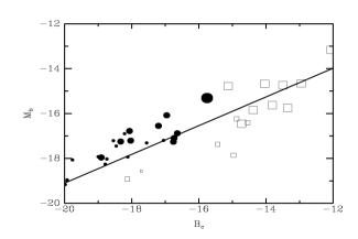
Figure 20: $M_{B}$ vs $B_{c}$ calibration. Black, solid dots represent objects from reference 19. Open squares are objects from references 13, 16, 17 and 18. Small symbols: galaxies further than $cz=3600$km s^-1. medium symbols: galaxies in the range $1800$km s^-1 $\leq cz\leq 3600$ km s^-1. Big symbols:galaxies nearer than 1800 km s^-1.

The color requirement was not straightforward to apply, because not many $B-V$ colors for the HII galaxies included in the sample were available in the literature. For this reason, a simple alternative method, based on spectroscopic criteria had to be developed.

The galaxy sample presented in Cairós et al. (2001a) and Cairós et al. (2001b) provides with $B-V$ colors for a sample of 28 blue compact galaxies, six of them appear in the Terlevich et al. (1991) catalogue. This smaller sample is shown in table 4.

Table 4: Galaxies used to re-define the color-criterium. Notes: (a) For Mrk370 and IIZw71 this number is defined as $1.3\times W_{5007}$; (b) This is the reddening-corrected $I_{\lambda}/I_{\beta}$ ratio; (1) Given values are $H\beta$weighted averages of the different zones defined in the respective papers; (2) Integrated spectrophotometry.

Object	B-V	ref	[OII]$\lambda 3727$(b)	[OIII]$\lambda 5007$(b)	$W_{3727}$	$W_{\beta}$	$W_{4959+5007}$(a)
Tol0127-397	0.56	Terlevich et al. (1991)	3.278	2.164	73	38	130
UM417	0.36	Terlevich et al. (1991)	0.330	5.566	20	144	903
Mrk370(1)	0.48	Cairós et al. (2002)	2.803	1.678	60.7	17.0	37.5
IIZw40	0.52	Terlevich et al. (1991)	0.440	7.76	79	268	2122
Mrk36	0.39	Terlevich et al. (1991)	0.988	5.506	42	70	432
UM462(1)	0.47	Terlevich et al. (1991)	1.777	5.320	96.1	102	615.8
IIZw71(2)	0.55	Jansen et al. (2000)	4.397	2.49	33.2	7.5	22.53

The adopted approach is to derive a least-squares fit to the observed colors as a function of the continuum strength ratio $x=\frac{\hbox{[OIII]}\lambda 5007\times W_{3727}}{\hbox{[OII]}\lambda 3727\times W_{4959+5007}}$. The fit is:

$$B-V=(0.54\pm 0.04)+(0.35\pm 0.16)\log x$$

Using this expression, the color condition is translated into $1.57\leq x$, which is the condition applied.

Unfortunately, not all references report the observed equivalent widths of the two oxygen lines required. Again, only the Terlevich et al. (1991) catalogue provides all the information.

However, all the objects from Terlevich et al. (1991) which show [OIII]$\lambda 4363$ included in the presented sample meet this requirement, and 96% of the objects without the auroral line from the Terlevich et al. (1991) sample also match the condition. Therefore, it is assumed that all the HII galaxies studied satisfy this condition.

This is not surprising, since the objects presented here were selected from objective prism surveys searching for either strong emission lines or UV excesses. The Tololo and UM surveys, looking for strong lined objects will pick up very blue objects, or compact starbursts with a weak continuum due to the presence of massive, young blue stars. The Markarian or Byurakan surveys, searching for galaxies presenting a UV excess naturally select blue objects. In addition, in these surveys, the photographic plates were more blue sensitive.

Unfortunately, no constraint on the surface brightness or half-light radius can be used with the data at hand. Galaxies satisfying the first two criteria are said to belong to the LCBG-like sample.

In total, 50 objects from subsample Sub1 and 117 sources from the subsample Sub2 were selected. These 167 objects are considered to be LCBG-like HII galaxies.

5.2 Properties of LCBG-like objects.

The aim of this work is to see where LCBG-like sources properties fit within the frame of HII galaxies in general. In order do this, the distributions of several quantities were drawn. Figures 21 to 28 give the corresponding distributions of the quantities.

Figure 21: Radial velocity distributions.

Figure 22: Observed H$\beta$ flux distributions.

Figure 23: H$\beta$ luminosity distributions.

Figure 24: Mass of the ionizing cluster distributions.

Figure 25: c(H$\beta$) distributions.

Figure 26: W_β distributions.

Figure 27: Ionization ratio distributions.

Figure 28: Metallicity distributions.

Figure 21 indicates that LCBG-like HII galaxies are mainly found at large distances. Only a tiny fraction of LCBG-like sources is located at redshifts lower than $\sim 0.01$, while this is the median value of the redshift distribution for less luminous systems. Figure 22 shows that the observed H$\beta$ flux distribution from LCBG-like objects is remarkably similar to that of the whole sample. In figure 23 it is seen that almost all LCBG-like galaxies have H$\beta$ luminosities greater than $10^{40}$erg s^-1. Only around 20 normal HII galaxies out of 242 are found with line luminosities greater than $10^{41}$erg s^-1. This suggests that a line luminosity around $3\times 10^{40}$erg s^-1 might be considered as the cut-off for HII galaxies similar to LCBG. This is a very important difference, since it means that this bright subsample of HII galaxies is powered by a greater number of stars. This is confirmed in figure 24, which presents the $\log M_{*}$ distribution for both samples. It is seen that LCBG-like HII galaxies have ionizing cluster masses greater than $10^{6}M_{\odot}$. Only 20 lower-luminosity HII galaxies have clusters that massive. However, since the calculated masses are only lower limits to the actual values due to photon-escape, presence of dust and the systematic error in the starburst equivalent width introduced by the underlying, non-ionizing population (partially corrected for by the use of the upper envelope of the W_β vs. $\log(\mbox{[OIII]/[OII]})$ presented in figure 6), LCBG-like HII galaxies will harbor ionizing cluster much more massive than this limit. This is the single, most important difference between LCBG-like HII galaxies and lower luminosity systems. The extinction distribution, shown in figure 25, indicates that there is a lack of LCBG-like sources with very low extinctions. At higher dust contents, c(H$\beta$)$\geq 0.30$, both distributions follow each other rather closely, though. This distribution also shows that bright HII galaxies are not affected by uncertainties in the extinction to a greater extent than the rest of the galaxies studied.

Figure 26 shows the existence of an upper limit to the equivalent width of the more luminous systems of around 200Å. The median values are 46.5Å for the LCBG-like subsample and 77.5Å for the rest of less luminous systems. These numbers show that large equivalent widths are mainly found among low luminosity HII galaxies and young starburst ages. Therefore, LCBG-like HII galaxies have probably built larger underlying stellar populations. This is further supported by the fact that the LCBG-like histogram shows a higher occupation number at very low equivalent widths. Figure 27 shows that the excitation is lower in LCBG-like HII galaxies. This suggests that the ionizing star clusters of LCBG-like HII galaxies are probably more evolved than those of less luminous HII galaxies. The oxygen abundance of LCBG-like systems compared to the whole sample can be seen in figure 28. This plot shows that there is a slight bias in the metal content. LCBG-like galaxies never show oxygen abundances lower than 7.6. At the same time, a very metal-rich object is more likely to be a LCBG-like galaxy. However, there seems to be no relationship between metallicity and luminosity since LCBG-like galaxies span pretty much the same metallicity range as the bulk of the whole sample of HII galaxies. In addition, figure 28 shows that the observed differences in the distributions of the ionization ratio shown in figure 27 can’t arise from a metallicity effect.

It is also enlightening to see whether LCBG-like galaxies are similar to HII galaxies with [OIII]$\lambda 4363$, or if they resemble HII galaxies without the auroral line. In order to do this, the dot product between the LCBG-like subsample and both Sub1 and Sub2 subsamples probability densities presented above (i.e. the histograms) were derived. Even though the probability densities for subsamples Sub1 and Sub2 are not orthogonal for any property studied, this should indicate which subsample is more similar to LCBG-like galaxies.

Table 5: Normalised dot products between LCBG-like subsample histograms and subsamples Sub1 and Sub2 probability densities.

Property.	With	Without
Bc	0.622	1.228
L$H\beta$	0.911	1.085
$\log$[OIII]/[OII]	0.560	0.955
c(H$\beta$)	0.446	0.965
$W_{\beta}$	0.889	0.880
$\log M_{*}$	0.735	1.123
$12+\log(O/H)$	0.905	0.935

Table 5 clearly shows that LCBG-like sources are more similar to objects not showing the auroral line [OIII]$\lambda 4363$. This table indicates that if a distant LCBG does not show the [OIII]$\lambda 4363$ line, it is likely that this object will present a massive underlying stellar population, high metallicity and low ionization.

6 Summary and Conclussions.

We have conducted a statistical study of a very large spectroscopic sample of HII galaxies from the literature. We have compared galaxies with and without the [OIII]$\lambda 4363$ line, and we have defined a control sample which can be used to investigate the nature of LCBGs at intermediate z.

It has been found that H$\beta$ fluxes are larger for objects showing the [OIII]$\lambda 4363$ line, even though the H$\beta$ luminosity distributions for galaxies with and without the auroral line are very similar. This is in part because objects not showing the auroral line are more distant and their extinction is higher. However, it has been shown that the undetection of the [OIII]$\lambda 4363$ line is a real metallicity effect for at least some fraction of cases. Objects without the auroral line are about 0.4dex more metal rich than objects from subsample Sub1. The analysis of the [OIII]/[OII] to $12+\log(O/H)$ relationship reveals the existence of high-ionization, metal rich objects without the auroral line. Objects from the second subsample are found to harbour more massive star clusters, although the differences in excitation between the two subsamples indicates that subsample Sub2 sources are probably powered by somewhat older star clusters.

LCBG-like sources are clearly further away than the average local HII galaxy. The H$\beta$ luminosities of LCBG-like systems are much greater. This is a very important difference between the two subsamples. We have also found that their ionizing star clusters are more massive that those of lower luminosity HII galaxies. LCBG-like HII galaxies have been found to posses larger (and hence probably older) underlying populations, and their ionizing star clusters are also more evolved and massive. LCBG-like sources are marginally more metal-rich than the average HII galaxy, but not enough to explain the observed differences in the ionization ratio [OIII]/[OII].

We have also shown that LCBG-like sources are more similar to objects without the auroral line [OIII]$\lambda 4363$, implying that any local control sample designed to study high-redshift LCBGs is to be made of galaxies not showing the [OIII]$\lambda 4363$ line. If one observes a distant LCBG and is unable to detect the [OIII]$\lambda 4363$ line, it is likely that this object will present a massive underlying stellar population, high metallicity and low ionization.

References

- Cairós et al. (2001a) Cairós L. M., Vílchez J. M., González Pérez J. N., Iglesias-Páramo J., Caon N., 2001, ApJS, 133, 321
- Cairós et al. (2001b) Cairós L. M., Caon N., Vílchez J. M., González-Pérez J. N., Muñoz-Tuñón C., 2001, ApJS, 136, 393
- Cairós et al. (2002) Cairós L. M., Caon N., García-Lorenzo B., Vílchez J. M., Muñoz-Tuñón C., 2002, ApJ, 577, 164
- Castellanos et al. (2002) Castellanos M., Díaz A. I., Terlevich E., 2002, MNRAS, 329, 315
- Denicoló et al (2002) Denicoló G., Terlevich R., Terlevich E., 2002, MNRAS, 330, 69
- Dennefeld & Stasinska (1983) Dennefeld M., Stasinska G.,1983, A&A, 118, 234
- Díaz et al. (1987) Díaz A. I., Terlevich E., Pagel B. E. J., Vilchez J. M., Edmunds M. G., 1987, MNRAS, 226, 19
- Díaz (1994) Díaz A. I., 1994, in Tenorio-Tagle G., eds Violent Star Formation, from 30 Doradus to QSOs. University Press, Cambridge, p. 105
- Díaz (1999) Díaz A. I., 1999, Ap&SS, 263, 143
- Dinerstein & Shields (1986) Dinerstein H. L., Shields G. A., 1986, ApJ, 311, 45
- French (1980) French H. B., 1980, ApJ, 240, 41
- García-Vargas et al. (1995) Garcia-Vargas M. L., Bressan A., Diaz A. I., 1995, A&AS, 112, 13
- Garnett et al. (1997) Garnett D. R., Shields G. A., Skillman E. D., Sagan S. P., Dufour R. J., 1997, ApJ, 489, 63
- Guseva et al. (2000) Guseva N. G., Izotov Y. I., Thuan T. X., 2000, ApJ, 531, 776
- Guzmán et al. (1997) Guzmán R., Gallego J., Koo D. C., Phillips A. C., Lowenthal J. D., Faber S. M., Illingworth G. D., Vogt N. P., 1997, ApJ, 489, 559
- Guzmán et al. (1998) Guzmán R., Jangren A., Koo D. C., Bershady M. A., Simard L., 1998, ApJ, 495, L13
- Hagen et al. (1995) Hagen H.-J., Groote D., Engels D., Reimers D., 1995, A&AS, 111, 195
- Hoyos et al. (2004) Hoyos C., Guzmán R., Bershady M. A., Koo D. C., Díaz A. I., 2004, AJ, 128, 1541
- Izotov et al. (1994) Izotov Y. I., Thuan T. X., Lipovetsky V. A., 1994, ApJ, 435, 647
- Izotov et al. (1997) Izotov Y. I., Thuan T. X.,Lipovetsky V. A., 1997, ApJS, 108, 1
- Izotov & Thuan (1998) Izotov Y. I., Thuan T. X., 1998, ApJ, 500, 188
- Jansen et al. (2000) Jansen R. A., Fabricant D., Franx M., Caldwell N., 2000, ApJS, 126, 331
- Kewley & Dopita (2002) Kewley L. J., Dopita M. A., 2002, ApJS, 142, 35
- Kinkel & Rosa (1994) Kinkel U., Rosa M. R., 1994, A&A, 282, L37
- Koo et al. (1994) Koo D. C., Bershady M. A., Wirth G. D., Stanford S. A., Majewski S. R., 1994, ApJ, 427, L9
- Kunth & Sargent (1983) Kunth D., Sargent W. L. W.,1983, ApJ, 273, 81
- Lequeux et al. (1979) Lequeux J., Peimbert M., Rayo J. F., Serrano A., Torres-Peimbert S., 1979,A&A, 80, 155
- MacAlpine, Lewis, & Smith (1977) MacAlpine G. M., Lewis D. W., Smith S. B., 1977, ApJS, 35, 203
- Markarian (1967) Markarian B. E., 1967, Afz, 3, 24
- Markarian, Lipovetskii, & Stepanian (1983) Markarian B. E., Lipovetskii V. A., Stepanian D. A., 1983, Afz, 19, 221
- Masegosa et al. (1994) Masegosa J., Moles M., Campos-Aguilar A., 1994, ApJ, 420, 576
- Maza et al. (1989) Maza J., Ruiz M. T., Gonzalez L. E., Wischnjewsky M., 1989, ApJS, 69, 349
- Melnick et al. (1992) Melnick J., Heydari-Malayeri M., Leisy P., 1992, A&A, 253, 16
- Melnick, Terlevich, & Moles (1985) Melnick J., Terlevich R., Moles M., 1985, RMxAA, 11, 91
- Mihalas (1972) Mihalas D., 1972, Non-LTE Model Atmospheres for B & O Stars, NCAR-TN/STR-76.
- Moles et al. (1990) Moles M., Aparicio A., Masegosa J., 1990, A&A, 228, 310
- Osterbrock (1989) Osterbrock D. E., 1989, Astrophysics of Gaseous Nebulae and Active Galactic Nuclei, (Mill Valley:University Science Books)
- Pagel et al. (1992) Pagel B. E. J., Simonson E. A., Terlevich R. J., Edmunds M. G., 1992, MNRAS, 255, 325
- Pastoriza et al. (1993) Pastoriza M. G., Dottori H. A., Terlevich E., Terlevich R., Diaz A. I., 1993, MNRAS, 260, 177
- Peña et al. (1991) Peña M., Ruiz M. T., Maza J., 1991, A&A, 251, 417
- Pérez-Montero & Díaz (2003) Pérez-Montero E., Díaz A. I., 2003, MNRAS, 346, 105
- Pérez-Montero, & Díaz (2005) Pérez-Montero, E., & Díaz A.I., 2004, submitted.
- Pesch & Sanduleak (1983) Pesch P., Sanduleak N., 1983, ApJS, 51, 171
- Phillips et al. (1997) Phillips A. C., Guzman R., Gallego J., Koo D. C., Lowenthal J. D., Vogt N. P., Faber S. M., Illingworth G. D., 1997, ApJ, 489, 543
- Pilyugin (2000) Pilyugin L. S., 2000, A&A, 362, 325
- Pilyugin (2001) Pilyugin L. S., 2001, A&A, 369, 594
- Popescu & Hopp (2000) Popescu C. C., Hopp U., 2000, A&AS, 142, 247
- Rayo et al. (1982) Rayo J. F., Peimbert M., Torres-Peimbert S., 1982, ApJ, 255, 1
- Salzer et al. (1995) Salzer J. J., Moody J. W., Rosenberg J. L., Gregory S. A., Newberry M. V., 1995, AJ, 109, 2376
- Searle & Sargent (1972) Searle L., Sargent W. L. W., 1972, ApJ, 173, 25
- Skillman (1989) Skillman E. D., 1989, ApJ, 347, 883
- Skillman & Kennicutt (1993) Skillman E. D., Kennicutt R. C., 1993, ApJ, 411, 655
- Skillman et al. (1994) Skillman E. D., Televich R. J., Kennicutt R. C., Garnett D. R., Terlevich E., 1994, ApJ, 431, 172
- Smith, Aguirre, & Zemelman (1976) Smith M. G., Aguirre C., Zemelman M., 1976, ApJS, 32, 217
- Stasińska, Schaerer, & Leitherer (2001) Stasińska G., Schaerer D., Leitherer C., 2001, A&A, 370, 1
- Terlevich & Melnick (1981) Terlevich R., Melnick J., 1981, MNRAS, 195, 839
- Telles et al. (1997) Telles E., Melnick J., Terlevich R., 1997, MNRAS, 288, 78
- Terlevich et al. (1991) Terlevich R., Melnick J., Masegosa J., Moles M., Copetti M. V. F., 1991, A&AS, 91, 285
- Thuan et al. (1995) Thuan T. X., Izotov Y. I., Lipovetsky V. A., 1995, ApJ, 445, 108
- Vilchez et al. (1988) Vilchez J. M., Pagel B. E. J., Diaz A. I., Terlevich E., Edmunds M. G., 1988, MNRAS, 235, 633