Performance Tuning of $N$-Body Codes on Modern Microprocessors:
I. Direct Integration with a Hermite Scheme on x86_64 Architecture

Abstract

The main performance bottleneck of gravitational $N$-body codes is the force calculation between two particles. We have succeeded in speeding up this pair-wise force calculation by factors between two and ten, depending on the code and the processor on which the code is run. These speedups were obtained by writing highly fine-tuned code for x86_64 microprocessors. Any existing $N$-body code, running on these chips, can easily incorporate our assembly code programs.

In the current paper, we present an outline of our overall approach, which we illustrate with one specific example: the use of a Hermite scheme for a direct $N^{2}$ type integration on a single 2.0 GHz Athlon 64 processor, for which we obtain an effective performance of 4.05 Gflops, for double precision accuracy. In subsequent papers, we will discuss other variations, including the combinations of $N\log N$ codes, single precision implementations, and performance on other microprocessors.

1 Introduction

Some $N$-body simulations can be sped up in various ways, by using faster algorithms such as tree codes (Barnes and Hut, 1986) and/or special purpose hardware such as the GRAPE family (Sugimoto et al., 1990). For some regimes, such as low $N$ values, these speed-up methods are not very efficient, and it would be nice to find other ways to improve the speed of such calculations. It would be even better if these alternative ways can be combined with other methods of speed-up.

We explore here a general approach based on speeding up the inner loop of gravitational force calculations, namely the interactions between one pair of particles. Also when using tree codes this approach will be useful, since in that case the calculation cost is still dominated by force calculations. Even for GRAPE applications, this approach will still be useful in many cases, since there are always some calculations which are done more efficiently on the front end.

In particular, we consider the optimization of the inner force loop on the x86-64 (or AMD64 or EM64T) architecture, the newest incarnation of the architecture that originated with the Intel 8080 microprocessor. Processors with an x86-64 instruction set are currently the most widely used. Athlon 64 and Opteron microprocessors from AMD, and many recent models of Pentium 4 and Xeon microprocessors from Intel, support this instruction set.

As will be shown in section 2, a straightforward implementation of the inner force loop using either Fortran or C, compiled with standard compilers like GCC or icc for x86-64 processors, results in a performance that is significantly lower than the theoretical peak value one can expect from the hardware. In the following, we discuss how we can improve the performance of the force loop on processors with an x86-64 instruction set.

1.1 The SSE2 Instruction Set

Our approach is based on the use of new features added to the x86 microprocessors in the last eight years. The first one is the SSE2 instruction set for double-precision floating-point arithmetic. Traditionally, the instruction set for x86 microprocessors has included the so-called x87 instruction set, which was originally designed for the 8087 math coprocessor for the 8086 16-bit microprocessor. This instruction set is stack-based, in the sense that it does not have any explicit way to specify registers. Instead, registers are indirectly accessed as a stack, where two operands for an arithmetic operation are taken from the top of the stack (popped) and the result is placed back at the top of the stack (pushed). Memory access also takes place through the top of the stack.

This x87 instruction set had the advantage that the instructions are simple and few in number, but for the last fifteen years the design of a fast floating-point unit for this x87 instruction set has been a major problem for all x86 microprocessors. If one would really design stack-based hardware, any pipelining would be practically impossible. In order to allow pipelining, current x86-based microprocessors, from Intel as well as AMD, translate the stack-based x87 instructions to RISC-like, presumably standard three-address register-to-register instructions in hardware at execution time.

This approach has given quite high performance, certainly much higher than what would have been possible with the original stack-based implementation. However, it was clear that pipelining and better use of hardware registers would be much easier if one could use an instruction set with explicit reference to the registers. In 2001, with the introduction of Pentium 4 microprocessors, Intel added such a new floating-point instruction set, which is called SSE2. It is still not a real three-address instruction set; it rather uses a two-address form where the address of the source register and that of the destination register are the same. Moreover, SSE2 still supports operations between the data in the main memory and that in the register, as was the case with the IBM System/360. Thus, it still has the look and feel of an instruction set from the 1960s.

1.2 Minimizing Memory Access

Even though operations between operands in memory and operands in registers are supported, clearly execution would be much faster if all operands could reside in registers. However, with the original SSE2 instruction set it was difficult to eliminate memory access for intermediate results, because there were only eight registers available for SSE2 instructions. For whatever reason, these registers are called “XMM” registers in the manufacturer’s document, and we follow this convention. With the new x86_64 instruction set, the number of these “XMM” registers was doubled from 8 to 16. The implication for $N$-body calculations was that it now became possible to minimize memory access during the inner force loop. A form of optimization using this approach will be discussed in section 3.

1.3 Exploiting Two-Word Double-Precision Parallelism

Another important feature of SSE2 (which is actually Streaming SIMD extension 2) is that it is defined to operate on a pair of two 64-bit floating point words, instead of a single floating-point word. This effectively means that the use of SSE2 instructions automatically result in the execution of two floating-point operations in parallel. While this feature cannot be easily used with any compiler-based optimization, it is possible to gain considerable profit from this feature through judicious hand coding. We discuss the use of this parallel nature of the SSE2 instruction set in section 4.

1.4 Exploiting Four-Word Single-Precision Parallelism

SSE2 is not the only new floating-point instruction set that has been made available for the x86 hardware. As the name SSE2 already suggests, there is an earlier SSE instruction set, which is similar to SSE2 but works only on single-precision floating-point numbers. As is the case with SSE2, SSE also works on multiple data in parallel, but instead of the two double-precision data of SSE2, SSE works on four single-precision floating-point numbers simultaneously. Thus, the peak calculation speed of SSE is at least a factor of two higher than that of SSE2. For those force calculations where single precision gives us a sufficient degree of accuracy, we can make use of SSE, gaining a performance that is even higher than what would have been possible with SSE2, as we discuss in section 5.

1.5 Utilizing Built-In Inverse Square Root Instructions

SSE was designed mainly to speed up coordinate transformation in three-dimensional graphics. As a result, it has a special instruction for the very fast calculation of an approximate inverse square root, which is intended as a good initial value for Newton-Raphson iteration. This is exactly what we need for the calculation of gravitational forces. We discuss the use of this approximate inverse square root for double-precision calculation, in section 4.

1.6 Organization

This paper is organized as follows. In section 2, we give the standard C-language implementation of the force loop. We consider the code fragment which calculates both the acceleration and its first time derivative. It is used with Hermite integration scheme (Makino & Aarseth, 1992).

We present the assembly language output and measured performance, and describe possible room for improvements. We call these implementations the baseline implementation.

In section 3, we discuss the optimized C-language implementation of the force loop for the Hermite scheme. The difference from the baseline implementation is that the C-language code is hand-tuned so that the load and store of intermediate results are eliminated from the generated assembly-language output. This version gives us the speed-up of 46% compared to the baseline method.

In section 4, we discuss a more efficient use of SSE2 instruction, where forces on two particles are calculated in parallel using the SIMD nature of the SSE2 instruction set. Here, we use the intrinsic data types defined in GCC, which allows us to use this SIMD nature within the syntax of C-language. Also, we use the fast approximate square root instruction and a Newton-Raphson iteration. This implementation is 88% faster than baseline.

In section 5, we discuss a mixed SSE-SSE2 implementation of the force calculation for the Hermite scheme. In many applications, full double-precision accuracy is not necessary, except for the first subtraction between positions and final accumulation of the forces. ”High-accuracy” GRAPE hardwares (GRAPE-2, 4 and 6) rely on this mixed-accuracy calculation. Thus, it is possible to perform most of the force-calculation operations using SSE single-precision instructions, thereby further speeding up the force calculation. In this way, we can speed-up the calculation by another 67 % from the SSE2 parallel implementation of section 4, achieving 219% speedup (3.19 times faster) from the baseline implementation.

2 Baseline implementation

2.1 Target functions

The target functions that we want to calculate are:

$${\bf a}_{i} = \sum_{j}{m_{j}{\bf r}_{ij}\over(r_{ij}^{2}+\varepsilon^{2})^{3/2}}$$ (1)

$${\bf j}_{i} = {{\bf{\dot{a}}}_{i}}\ =\ \sum_{j}m_{j}\left[{{\bf v}_{ij}\over(r_{ij}^{2}+\varepsilon^{2})^{3/2}}-{3({\bf v}_{ij}\cdot{\bf r}_{ij}){\bf r}_{ij}\over(r_{ij}^{2}+\varepsilon^{2})^{5/2}}\right]$$ (2)

$$\phi_{i} = -\sum_{j}{m_{j}\over(r_{ij}^{2}+\varepsilon^{2})^{1/2}}$$ (3)

where ${\bf a}_{i}$ and $\phi_{i}$ are the gravitational acceleration and the potential of particle $i$, the jerk ${\bf j}_{i}$ is the time derivative of the acceleration, and ${\bf r}_{i}$, ${\bf v}_{i}$, and $m_{i}$ are the position, velocity and mass of particle $i$, ${\bf r}_{ij}={\bf r}_{j}-{\bf r}_{i}$ and ${\bf v}_{ij}={\bf v}_{j}-{\bf v}_{i}$.

The calculation of ${\bf a}$ and $\phi$ requires 9 multiplications, 10 addition/subtraction operations, 1 division and 1 square root calculation. Clearly, calculation of an inverse square root is more expensive than addition/multiplication operations. Therefore, if we want to measure the speed of a force calculation loop in terms of the number of floating-point operations per second, we need to introduce some conversion factor for division and square root calculations. In this paper, we use 38 as the total number of floating point operations for the calculation of ${\bf a}$ and $\phi$. This implies that we effectively assign around 10 operations to each division and to each square root calculation. This particular convention was introduced by Warren et al. (1997), and we follow it here since it seems to be a reasonable representation of the actual computational costs of force calculations on typical scalar processors.

In addition, it requires 11 multiplications and 11 addition/subtraction operations to calculate ${\bf j}$. Thus, the total number of floating-point operations per inner force loop for the Hermite scheme can be given as 60. This is the number that we will use here. Note that we have previously used numbers that were slightly less, by about 5%, using 57 instead of 60 (Makino et al., 2001).

In the case of a simple leapfrog method or traditional ”Aarseth” scheme, we need to calculate only ${\bf a}_{i}$ and $\phi_{i}$. For a Hermite scheme we need to determine ${\bf j}_{i}$ as well.

2.2 Baseline implementation and its performance

The following code fragments contain what we regard as the baseline implementation of the force calculations, where we use the word ‘force’ loosely, to indicate the calculations for accelerations, jerks as well as the potential. In other words, we consider ‘force calculations’ to comprise all the basic low-level dynamical calculations governing the interactions between pairs of particles.

List 1: Baseline implementation calculates force on $i$th particle.

⬇

1#define DIM 3

2

3typedef struct{

4 double x[DIM];

5 double v[DIM];

6 double m;

7}Predictor;

8typedef Predictor * pPredictor;

9

10typedef struct{

11 double a[DIM];

12 double j[DIM];

13 double pot;

14}AccJerk;

15typedef AccJerk * pAccJerk;

16

17void CalcAccJerk_Base (pPredictor pr, pAccJerk aj,

18 double eps2, int i, int nbody){

19 int j, k;

20 double r[3], v[3], acc[3], jerk[3], pot;

21 double r2, rv;

22 double rinv,rinv2;

23 double mrinv, mrinv3, rvrinv2;

24

25 pot = 0.0;

26 for(k=0; k<3; k++) acc[k] = jerk[k] = 0.0;

27

28 for(j=0; j<nbody; j++){

29 if(j == i) continue;

30 for(k=0; k<3; k++){

31 r[k] = pr[j].x[k] - pr[i].x[k];

32 v[k] = pr[j].v[k] - pr[i].v[k];

33 }

34

35 r2 = eps2;

36 for(k=0; k<3; k++) r2 += r[k] * r[k];

37 rv = r[0] * v[0];

38 for(k=1; k<3; k++) rv += r[k] * v[k];

39

40 rinv2 = 1./r2;

41 rinv = sqrt(rinv2);

42 rvrinv2 = 3.0 * rv * rinv2;;

43 mrinv = rinv * pr[j].m;

44 mrinv3 = mrinv * rinv2;

45

46 pot -= mrinv;

47

48 for(k=0; k<3; k++){

49 double temp = r[k] * mrinv3;

50 acc [k] += temp;

51 jerk[k] += v[k] * mrinv3 - temp * rvrinv2;

52 }

53 }

54

55 for(k=0; k<3; k++){

56 aj->a[k] = acc[k];

57 aj->j[k] = jerk[k];

58 aj->pot = pot;

59 }

60}

Line 29 in list 1 is a branch to avoid self interaction. We might remove this branch when we can use softening, but in this case branch prediction of the microprocessor works ideally, hence the performance changes little if we remove this.

Table 1: Performance of the code shown in list 1 when $N=1024$, in cycles-per-interaction and Gflops, on Athlon 64 2.0GHz.

Compiler	Options	Cycles	Gflops
GCC 3.3.1	-O3 -ffast-math -funroll-loops	94.8	1.27
GCC 3.3.1	-O3 -ffast-math -funroll-loops -mfpmath=387	119	1.01
GCC 4.0.1	-O3 -ffast-math -funroll-loops	100	1.20
PGI 5.1	-fastsse	97.6	1.23
PathScale 2.0	-O3 -ffast-math	95.0	1.26
ICC 9.0	-O3	95.8	1.25

Table 1 shows the performance of this code on an AMD Athlon 64 3000+ (2.0GHz) processor with several different compilers. The first column gives the compiler used, the second the compiler options, the third the clock cycles per pairwise force calculation, and the fourth column gives the speed in Gflops. All compilers generate SSE2 instructions instead of x87 instructions unless we explicitly set options to use x87. The performance is fairly good, but not ideal. In the following we will investigate how we can improve the performance.

List 2 is the assembly language output of the Hermite force loop using the GCC compiler:

List 2: Assembly output of list 1 using GCC 3.3.1 with option -S -O3 -ffast-math -funroll-loops, commented by the authors for clarity.

⬇

1 xorpd %xmm9, %xmm9

2 xorl %r8d, %r8d

3 subq $16, %rsp

4.LCFI0:

5 movsd %xmm0, %xmm10

6 movl %edx, %r11d

7 cmpl %ecx, %r8d

8 movl %ecx, %r10d

9 movsd %xmm9, -120(%rsp)

10 movsd %xmm9, -88(%rsp)

11 movsd %xmm9, -112(%rsp)

12 movsd %xmm9, -80(%rsp)

13 movsd %xmm9, -104(%rsp)

14 movsd %xmm9, -72(%rsp)

15 jge .L41

16 movslq %edx,%rdx

17 movlpd .LC4(%rip), %xmm11

18 movlpd .LC5(%rip), %xmm12

19 leaq 0(,%rdx,8), %r9

20 subq %rdx, %r9

21 .p2align 4,,7

22.L60:

23 cmpl %r11d, %r8d

24 je .L9 # continue

25 movslq %r8d,%rcx

26 leaq 0(,%rcx,8), %rdx

27 subq %rcx, %rdx # %rdx = 7 * %rcx

28 leaq 8(,%r9,8), %rcx

29 movlpd (%rdi,%rdx,8), %xmm6 # %xmm6 = pr[j].x[0]

30 leaq 8(,%rdx,8), %rax

31 subsd (%rdi,%r9,8), %xmm6 # %xmm6 -= pr[i].x[0]

32 movsd %xmm6, -24(%rsp) # *(%rsp-24) = %xmm6

33 movsd %xmm6, %xmm3

34 movlpd 24(%rdi,%rdx,8), %xmm4

35 subsd 24(%rdi,%r9,8), %xmm4 # %xmm4 = pr[j].v[0] - pr[i].v[0]

36 mulsd %xmm6, %xmm3 # %xmm3 = x*x

37 addsd %xmm10, %xmm3 # %xmm3 += eps2

38 movsd %xmm4, -56(%rsp)

39 movlpd (%rdi,%rax), %xmm7

40 subsd (%rdi,%rcx), %xmm7 # %xmm7 = pr[j].x[1] - pr[i].x[1]

41 movsd %xmm7, -16(%rsp)

42 movsd %xmm7, %xmm15

43 movsd %xmm7, %xmm2

44 movlpd 24(%rdi,%rax), %xmm14

45 leaq 16(,%rdx,8), %rax

46 subsd 24(%rdi,%rcx), %xmm14 # %xmm14 = pr[j].v[1] - pr[i].v[1]

47 mulsd %xmm7, %xmm15

48 leaq 16(,%r9,8), %rcx

49 addsd %xmm15, %xmm3 # %xmm3 += y*y

50 movlpd -88(%rsp), %xmm15 # load acc[0]

51 movsd %xmm14, -48(%rsp)

52 mulsd %xmm14, %xmm2

53 movlpd (%rdi,%rax), %xmm8

54 subsd (%rdi,%rcx), %xmm8 # %xmm8 = pr[j].x[2] - pr[i].x[2]

55 movsd %xmm8, %xmm5

56 movsd %xmm8, -8(%rsp)

57 movsd %xmm8, %xmm0

58 movlpd 24(%rdi,%rax), %xmm13

59 mulsd %xmm8, %xmm5

60 subsd 24(%rdi,%rcx), %xmm13 # %xmm13 = pr[j].v[2] - pr[i].v[2]

61 addsd %xmm5, %xmm3 # %xmm3 += z*z

62 movsd %xmm6, %xmm5

63 mulsd %xmm4, %xmm5 # %xmm5 = x*vx

64 movsd %xmm13, -40(%rsp)

65 mulsd %xmm13, %xmm0

66 addsd %xmm2, %xmm5 # %xmm5 += y*vy

67 movsd %xmm11, %xmm2 # %xmm2 = 1.0

68 divsd %xmm3, %xmm2 # %xmm2 = 1.0/r2

69 movlpd -80(%rsp), %xmm3

70 addsd %xmm0, %xmm5 # %xmm5 += z*vz

71 sqrtsd %xmm2, %xmm1 # %xmm1 = 1.0/r

72 mulsd %xmm2, %xmm5 # %xmm5 = rv/r2

73 mulsd 48(%rdi,%rdx,8), %xmm1 # %xmm1 *= pr[j].m

74 mulsd %xmm12, %xmm5 # %xmm5 = 3rv/r2

75 mulsd %xmm1, %xmm2 # %xmm2 = m/r3

76 subsd %xmm1, %xmm9 # pot -= m/r

77 movlpd -72(%rsp), %xmm1

78 mulsd %xmm2, %xmm6

79 mulsd %xmm2, %xmm7

80 mulsd %xmm2, %xmm8

81 mulsd %xmm2, %xmm4

82 addsd %xmm6, %xmm15 # acc[0] += x[0] * m/r3

83 mulsd %xmm2, %xmm14

84 addsd %xmm7, %xmm3

85 mulsd %xmm5, %xmm6

86 addsd %xmm8, %xmm1

87 mulsd %xmm5, %xmm7

88 mulsd %xmm2, %xmm13

89 mulsd %xmm5, %xmm8

90 movsd %xmm15, -88(%rsp) # store acc[0]

91 subsd %xmm6, %xmm4

92 movsd %xmm3, -80(%rsp) # store acc[1]

93 subsd %xmm7, %xmm14

94 addsd -120(%rsp), %xmm4

95 movsd %xmm1, -72(%rsp) # store acc[2]

96 addsd -112(%rsp), %xmm14

97 subsd %xmm8, %xmm13

98 addsd -104(%rsp), %xmm13

99 movsd %xmm4, -120(%rsp) # store jerk[0]

100 movsd %xmm14, -112(%rsp) # store jerk[1]

101 movsd %xmm13, -104(%rsp) # store jerk[2]

102.L9:

103 incl %r8d

104 cmpl %r10d, %r8d

105 jl .L60 # if(++j < nbody) goto .L60:

106.L41:

107 movq -88(%rsp), %r11

108 movq -120(%rsp), %r10

109 movsd %xmm9, 48(%rsi)

110 movq -80(%rsp), %r9

111 movq -112(%rsp), %r8

112 movq -72(%rsp), %rdi

113 movq -104(%rsp), %rdx

114 movq %r11, (%rsi)

115 movq %r10, 24(%rsi)

116 movq %r9, 8(%rsi)

117 movq %r8, 32(%rsi)

118 movq %rdi, 16(%rsi)

119 movq %rdx, 40(%rsi)

120 addq $16, %rsp

121 ret

One can see that there are quite a few unnecessary load/store instructions. For example, the store instructions in lines 32, 38, 41, 51, 56 and 64 of list 2 serve no purpose. Also Arrays acc[3] and jerk[3] could be placed in registers like variable pot, but they are placed in memory instead.

3 C-level optimization

3.1 Code modification

As we have seen in the previous section, the assembly language output shows a significant amount of unnecessary load/store instructions. In principle, if the compilers were clever enough they would be able to eliminate these unnecessary operations. In practice, we need to guide the compilers so that they do not generate unnecessary code.

We have achieved significant speedup using the following two guiding principles:

1. Eliminate assignment to any array element in the force loop.

2. Reuse variables as much as possible in order to minimize the number of registers used.

Apparently, present-day compilers are not clever enough to eliminate load/store operations, if elements of arrays are used as left-hand-side values. Therefore, we hand-unroll all loops of length three and use scalar variables instead of arrays for three-dimensional vectors.

In well-written programs, variables which contain the values for different physical quantities should have different names. However, the use of many different names prevents optimization, since it results in a number of variables too large to be fitted into the register set of SSE2 instructions (there are 16 ”XMM” registers for SSE2 instructions). Therefore, we explicitly reuse variables such as x, y, z so that these can hold both the position difference components as well as the pairwise force components, at different times in the computation.

The resulted C-language code is the following:

List 3: An optimized force loop.

⬇

1typedef struct{

2 double x[3];

3 double v[3];

4 double m;

5 double pad;

6}Predictor;

7typedef Predictor * pPredictor;

8

9void CalcAccJerk_Fast (pPredictor pr, pAccJerk aj,

10 double eps2, int i, int nj){

11 int j;

12 double x,y,z,vx,vy,vz;

13 double ax,ay,az,jx,jy,jz,pot;

14 double r2,rv;

15 double rinv,rinv2,rinv3;

16 pPredictor jpr = pr;

17 pPredictor ipr = pr + i;

18

19 pot=ax=ay=az=jx=jy=jz=0.0;

20

21 for(j=0;j<nj;j++,jpr++){

22 __builtin_prefetch(jpr+2, 0, 3);

23 if(j == i) continue;

24 x = jpr->x[0] - ipr->x[0];

25 y = jpr->x[1] - ipr->x[1];

26 z = jpr->x[2] - ipr->x[2];

27

28 vx= jpr->v[0] - ipr->v[0];

29 vy= jpr->v[1] - ipr->v[1];

30 vz= jpr->v[2] - ipr->v[2];

31

32 r2 = eps2 + x*x + y*y + z*z;

33

34 rv = vx*x + vy*y + vz*z;

35

36 rinv2 = 1./r2;

37 rinv = sqrt(rinv2);

38 rv *= rinv2*3.;

39 rinv *= jpr->m;

40 rinv3 = rinv * rinv2;

41

42 pot -= rinv;

43

44 x *= rinv3; ax += x;

45 y *= rinv3; ay += y;

46 z *= rinv3; az += z;

47

48 vx *= rinv3; jx += vx;

49 vy *= rinv3; jy += vy;

50 vz *= rinv3; jz += vz;

51

52 x *= rv; jx -= x;

53 y *= rv; jy -= y;

54 z *= rv; jz -= z;

55 }

56

57 aj->a[0] = ax;

58 aj->a[1] = ay;

59 aj->a[2] = az;

60 aj->j[0] = jx;

61 aj->j[1] = jy;

62 aj->j[2] = jz;

63 aj->pot = pot;

64}

This code is compiled into the following assembly code using the GCC 3.3.1 compiler (flag -O3 -ffast-math):

List 4: Assembly output of list 3.

⬇

1CalcAccJerk_Fast:

2.LFB3:

3 movslq %edx,%r8

4 xorpd %xmm9, %xmm9

5 salq $6, %r8

6 movsd %xmm0, -8(%rsp)

7 leaq (%r8,%rdi), %rax

8 movsd %xmm9, %xmm11

9 movsd %xmm9, %xmm10

10 xorl %r8d, %r8d

11 movsd %xmm9, %xmm14

12 movsd %xmm9, %xmm13

13 cmpl %ecx, %r8d

14 movsd %xmm9, %xmm12

15 movsd %xmm9, %xmm15

16 jge .L9

17 .p2align 4,,7

18.L11:

19 cmpl %edx, %r8d

20 prefetcht0 128(%rdi)

21 je .L4

22 movlpd (%rdi), %xmm3

23 movlpd 8(%rdi), %xmm4

24 subsd (%rax), %xmm3

25 movlpd 16(%rdi), %xmm5

26 subsd 8(%rax), %xmm4

27 movlpd 24(%rdi), %xmm6

28 subsd 16(%rax), %xmm5

29 movlpd 32(%rdi), %xmm7

30 subsd 24(%rax), %xmm6

31 movlpd 40(%rdi), %xmm8

32 subsd 32(%rax), %xmm7

33 subsd 40(%rax), %xmm8

34 movsd %xmm3, %xmm0

35 movsd %xmm4, %xmm2

36 mulsd %xmm3, %xmm0

37 addsd -8(%rsp), %xmm0

38 mulsd %xmm4, %xmm2

39 movsd %xmm7, %xmm1

40 mulsd %xmm4, %xmm1

41 addsd %xmm2, %xmm0

42 movsd %xmm5, %xmm2

43 mulsd %xmm5, %xmm2

44 addsd %xmm2, %xmm0

45 movsd %xmm6, %xmm2

46 mulsd %xmm3, %xmm2

47 addsd %xmm1, %xmm2

48 movsd %xmm8, %xmm1

49 mulsd %xmm5, %xmm1

50 addsd %xmm1, %xmm2

51 movlpd .LC4(%rip), %xmm1

52 divsd %xmm0, %xmm1

53 sqrtsd %xmm1, %xmm0

54 mulsd %xmm1, %xmm2

55 mulsd 48(%rdi), %xmm0

56 mulsd .LC5(%rip), %xmm2

57 mulsd %xmm0, %xmm1

58 subsd %xmm0, %xmm15

59 mulsd %xmm1, %xmm3

60 mulsd %xmm1, %xmm4

61 mulsd %xmm1, %xmm5

62 mulsd %xmm1, %xmm6

63 mulsd %xmm1, %xmm7

64 addsd %xmm3, %xmm12

65 mulsd %xmm1, %xmm8

66 addsd %xmm4, %xmm13

67 addsd %xmm5, %xmm14

68 mulsd %xmm2, %xmm3

69 addsd %xmm6, %xmm10

70 mulsd %xmm2, %xmm4

71 addsd %xmm7, %xmm11

72 mulsd %xmm2, %xmm5

73 addsd %xmm8, %xmm9

74 subsd %xmm3, %xmm10

75 subsd %xmm4, %xmm11

76 subsd %xmm5, %xmm9

77.L4:

78 incl %r8d

79 addq $64, %rdi

80 cmpl %ecx, %r8d

81 jl .L11

82.L9:

83 movsd %xmm12, (%rsi)

84 movsd %xmm13, 8(%rsi)

85 movsd %xmm14, 16(%rsi)

86 movsd %xmm10, 24(%rsi)

87 movsd %xmm11, 32(%rsi)

88 movsd %xmm9, 40(%rsi)

89 movsd %xmm15, 48(%rsi)

90 ret

%xmm0	rinv, r2
%xmm1	rinv2, rinv3, y*vy, z*vz
%xmm2	rv, y*y, z*z
%xmm3	x
%xmm4	y
%xmm5	z
%xmm6	vx
%xmm7	vy
%xmm8	vz
%xmm9	jz
%xmm10	jx
%xmm11	jy
%xmm12	ax
%xmm13	ay
%xmm14	az
%xmm15	pot

Figure 1: The use of XMM registers in list 4.

Table 2: Performance of list 3 when $N=1024$, in cycles-per-interaction and Gflops, on Athlon 64 3000+ 2.0GHz.

Compiler	Options	Cycles	Gflops
GCC 3.3.1	-O3 -ffast-math	64.8	1.85
GCC 4.0.1	-O3 -ffast-math	64.7	1.85
ICC 9.0	-O3	79.4	1.51

We can see that now all load/store instructions of the intermediate results are eliminated. Figure 1 shows the use of registers and table 2 presents the performance data for this code. This version is 46% faster than the code in section 2. Very roughly, this speed-up is consistent with the reduction in the number of assembly language instructions (from 82 to 62), but is somewhat larger. This is partly because the instructions which take memory arguments have a larger latency than register-only instructions.

3.2 Prefetch insertion and alignment

Line 22 of list 3 shows a built-in function for GCC, which is compiled into a prefetch instruction. In this case, the prefetch instruction loads the data which will be needed two iterations after the current one. The second and third parameters are read/write flags for which zero indicates preparing for a read and the degree of temporal locality takes value from 1 to 3.

Line 6 of list 3 shows a pad to make the size of the predictor structure to be exactly 64-byte, which is the cache-line size of Athlon 64 processor. To make the predictor structure align at 64-byte boundary, we use memalign() or posix_memalign() instead of malloc().

Figure 2: Clock cycles per force calculation loop as a function of $N$ on Athlon 64 3000+ 2.0 GHz. Open squares and triangles show the results of using code with prefetch and with and without 64-byte alignment. Filled squares and triangles show the result of using code without prefetch and with and without 64-byte alignment.

Figure 2 shows the performance of the force loop as the function of the loop length $N$, with and without this prefetch instruction and 64-byte alignment. The fastest case depends on $N$. For the region $N\leq 1024$, in which data fits into 64 kB of L1 data cache, the code with prefetch and 64-byte alignment is the best. For larger $N$, the code with prefetch and without alignment is the best.

4 Assembly-level optimization

In this section, we give two extensions specialized for x86/x86_64 architecture for the force loop. The first is using SSE2 vector (SIMD) mode instead of SSE2 scalar (SISD) mode. The second is replacing one division and one square root, by a special instruction for fast approximate inverse square root in SSE and Newton-Raphson iteration.

4.1 SSE2 vector mode

In the previous section we improved the performance of the C-language implementation of the force loop, essentially by hand-optimizing the C code so that the generated assembly code becomes optimal. However, in this way, we did not use the full capability of SSE2. While SSE2 instructions can process two double-precision numbers in parallel, the force loop discussed in the previous section uses only one of these two words. Clearly, we did not yet use the ”SIMD” nature of the instruction set.

Whether or not we can gain by using this SIMD nature depends on the particular code, and also on the particular processor. On Intel P4 architecture the SIMD mode can offer up to a factor of two speedup, while on AMD Athlon 64 or Intel Pentium M, the speed increase can be small (or even negative).

There are many ways to use this SIMD feature. Since there are similarities with the vector instructions of some old vector processors, in particular the Cyber 205, one could make use of an automatic vectorizing compiler (such as icc version 6.0 and later). However, just as was the case with the old vectorizing compilers, the vectorizing capability of modern compilers are still very limited, and it is hard to rewrite the force loop so that the compiler can make use of the SIMD capability.

In fact, part of the reason why vectorization is difficult is that the load/store capability of SSE2 instructions is rather limited: it can work efficiently only on a pair of two double-precision words in consecutive and 16-byte aligned addresses. This means that the basic loop structure cannot work, and one needs to copy the data of two particles into some special data structure, in order to let the compiler generate the appropriate SIMD instructions.

Here we have adopted a low-level approach, in which we make use of the special data type of pairs of double precision words defined in GCC. Basically, this data type, which we call v2df, corresponds to what is in one XMM register (a pair of double-precision words). We can perform the usual arithmetic operations and even function calls for this data type. Here is the code which makes use of this v2df data type:

List 5: Defining SSE/SSE2 data type.

⬇

1typedef double v2df __attribute__ ((mode(V2DF)));

2typedef float v4sf __attribute__ ((mode(V4SF)));

The v4sf data type packs four single-precision words for SSE which we will use later.

The basic idea here is to calculate the forces from one particle on two different particles in parallel. One could try to calculate the forces from, rather than on, two different particles on one particle in parallel, but that would result in a more complicated program since then we will need to add up the two partial forces in the end. Also, from the point of view of memory bandwidth, our approach is more efficient, since we need to load only one particle per iteration. Note that this is the same approach as what is called $i$-parallelism in the various versions of GRAPE hardware, where parallel pipelines calculate the forces on different particles from the same set of particles.

In this code, we use macros for gathering load and scattering store using instructions for loading/storing the higher/lower half of an XMM register:

List 6: Gathering load and scattering store for SSE2.

⬇

1#define V2DF_GATHER(reg, ptr0, ptr1) \

2 reg = __builtin_ia32_loadlpd(reg, (void *)(ptr0)); \

3 reg = __builtin_ia32_loadhpd(reg, (void *)(ptr1));

4

5#define V2DF_SCATTER(reg, ptr0, ptr1) \

6 __builtin_ia32_storelpd((void *)(ptr0), reg); \

7 __builtin_ia32_storehpd((void *)(ptr1), reg);

We should be careful about the fact that these built-in functions are undocumented feature of GCC. The GCC document describes built-in functions for most SSE/SSE3 instructions but not for any of SSE2 instruction. We can call most SSE2 instruction through the prefix __builtin_ia32_. Note that, for whatever reason, instructions such as ”movxxx” from/to memory are changed to ”loadxxx”/”storexxx”. But this does not mean that GCC always generates correct assembly output. For example, GCC generates wrong code for the first macro in list 6 when reg is not a register variable. This can be considered either a bug or a feature, and it shows the risk of using these undocumented aspects of GCC.

We also use macros for numerical values since we cannot use numerical values like ”3.0” for vector operations:

List 7: Macros for numerical values.

⬇

1#define V2DF_OP_SCALAR(reg, op, imm) { \

2 v2df v2df_temp = {imm, imm}; \

3 reg op v2df_temp; \

4}

5#define V2DF_OP_VECTOR(reg, op, imm0, imm1) { \

6 v2df v2df_temp = {imm0, imm1}; \

7 reg op v2df_temp; \

8}

9#define V4SF_OP_SCALAR(reg, op, imm) { \

10 v4sf v4sf_temp = {imm, imm, imm, imm}; \

11 reg op v4sf_temp; \

12}

Note that we need to copy the data of a single particle into both high and low words of an XMM register. The new SSE3 extension supports this ”broadcasting”, while the original SSE2 set did not. Therefore, we use the following macro:

List 8: Broadcast loading for double precision.

⬇

1#ifdef __SSE3__

2#define LOADDDUP(reg, ptr) \

3 reg = __builtin_ia32_loadddup(ptr);

4#else

5#define LOADDDUP(reg, ptr) \

6 reg = __builtin_ia32_loadlpd(reg, (void *)(ptr)); \

7 reg = __builtin_ia32_loadhpd(reg, (void *)(ptr));

We show the vectorized force loop using these data types and macros in list 9.

List 9: Vectorized force loop using SSE2 vector mode.

⬇

1typedef struct{

2 double x[3];

3 double v[3];

4 double m[2];

5}Predictor;

6typedef Predictor * pPredictor;

7

8void CalcAccJerk_Vector (pPredictor pr, pAccJerk AccJerkOut,

9 double eps2, int index[], int nj){

10 int j, k;

11 v2df x,y,z,vx,vy,vz,ax,ay,az,jx,jy,jz,pot;

12 v2df r2,rv;

13 v2df rinv1,rinv2,rinv3;

14 static v2df zero = {0.0, 0.0};

15 pPredictor prj = pr;

16 int i0 = index[0];

17 int i1 = index[1];

18 v2df xi[7];

19 v2df *vi = xi+3;

20 v2df *eps2p = xi+6;

21

22 pot=ax=ay=az=jx=jy=jz = zero;

23

24 for(k=0;k<3;k++){

25 V2DF_OP_VECTOR(xi[k], =, pr[i0].x[k], pr[i1].x[k]);

26 V2DF_OP_VECTOR(vi[k], =, pr[i0].v[k], pr[i1].v[k]);

27 }

28 V2DF_OP_SCALAR(*eps2p, =, eps2);

29 for(j=0;j<nj;j++,prj++){

30 LOADDDUP(x, prj->x);

31 x -= xi[0];

32 LOADDDUP(y, prj->x+1);

33 y -= xi[1];

34 LOADDDUP(z, prj->x+2);

35 z -= xi[2];

36 LOADDDUP(vx, prj->v);

37 vx -= vi[0];

38 LOADDDUP(vy, prj->v+1);

39 vy -= vi[1];

40 LOADDDUP(vz, prj->v+2);

41 vz -= vi[2];

42

43 r2 = x*x + y*y + z*z + *eps2p;

44 rv = vx*x + vy*y + vz*z;

45 __builtin_prefetch(prj+2, 0, 3);

46

47 V2DF_OP_SCALAR(rinv2, =, 1.0);

48 rinv2 /= r2;

49 rinv1 = __builtin_ia32_sqrtpd(rinv2);

50

51 rv *= rinv2;

52 V2DF_OP_SCALAR(rv, *=, 3.0);

53

54 rinv1 *= *(v2df *)(prj->m);

55 pot -= rinv1;

56 rinv3 = rinv1 * rinv2;

57

58 x *= rinv3; ax += x;

59 y *= rinv3; ay += y;

60 z *= rinv3; az += z;

61

62 vx *= rinv3; jx += vx;

63 vy *= rinv3; jy += vy;

64 vz *= rinv3; jz += vz;

65

66 x *= rv; jx -= x;

67 y *= rv; jy -= y;

68 z *= rv; jz -= z;

69 }

70

71 { /* correct self interaction */

72 v2df mass = {pr[i0].m[0], pr[i1].m[0]};

73 V2DF_OP_SCALAR(mass, *=, 1.0/sqrt(eps2));

74 pot += mass;

75 }

76 V2DF_SCATTER(ax, AccJerkOut[0].a, AccJerkOut[1].a);

77 V2DF_SCATTER(ay, AccJerkOut[0].a+1, AccJerkOut[1].a+1);

78 V2DF_SCATTER(az, AccJerkOut[0].a+2, AccJerkOut[1].a+2);

79 V2DF_SCATTER(jx, AccJerkOut[0].j, AccJerkOut[1].j);

80 V2DF_SCATTER(jy, AccJerkOut[0].j+1, AccJerkOut[1].j+1);

81 V2DF_SCATTER(jz, AccJerkOut[0].j+2, AccJerkOut[1].j+2);

82 V2DF_SCATTER(pot, &AccJerkOut[0].pot, &AccJerkOut[1].pot);

83}

The predictor structure has changed to store the same mass value in two places (line 4), in order to save an instruction (line 54).

4.2 Fast approximate inverse square root

The most expensive part of the force calculation, for recent microprocessors, is the calculation of an inverse square root which requires one division and one square root caluclations. Several attempts to speed this up using table lookup, polynomial approximation and Newton-Raphson iteration have been reported (e.g. Karp 1992). The main difficulty in these approaches is how to get a good approximation for the starting value of a Newton-Raphson iteration quickly.

Here, we use RSQRTSS/PS instruction in the SSE instruction set, which provide approximate values for the inverse square root for scalar/vector single-precision floating-point numbers, to an accuracy of about 12 bits. With one Newton-Raphson iteration, we can obtain 24-bit accuracy, which is sufficient for most “high-accuracy” calculations. If higher accuracy is really necessary, we could apply a second iteration. The Newton-Raphson iteration formula is expressed as:

$$x_{1}=-\frac{1}{2}x_{0}(ax_{0}^{2}-3).$$ (4)

Here, $x_{0}$ is an initial guess for $1/\sqrt{a}$.

We show the implementation for a scalar version using inline assembly code with GCC extensions:

List 10: Calling rsqrtss through inline assembly code.

⬇

1 double r2, rinv;

2 float ftmp;

3

4 ftmp = (float)r2;

5 asm("rsqrtss␣%1,␣%0":"=x"(ftmp):"x"(ftmp));

6 rinv = (double)ftmp;

7 rinv *= r2*rinv*rinv - 3.0;

and for a vector version using built-in functions:

List 11: Calling rsqrtps using built-in functions of GCC.

⬇

1 v2df r2, rinv;

2 v4sf ftmp;

3

4 ftmp = __builtin_ia32_cvtpd2ps(r2);

5 ftmp = __builtin_ia32_rsqrtps(ftmp);

6 rinv = __builtin_ia32_cvtps2pd(ftmp);

7 r2 *= rinv;

8 r2 *= rinv;

9 V2DF_OP_SCALAR(r2, -= , 3.0);

10 rinv *= r2;

Note that we skip here the multiplication by $-1/2$ in equation (4). This can be done after the total force is obtained.

To use RSQRTSS/PS instructions, we first convert $r^{2}$ into single precision, then apply these instructions, and finally convert the result back to double precision.

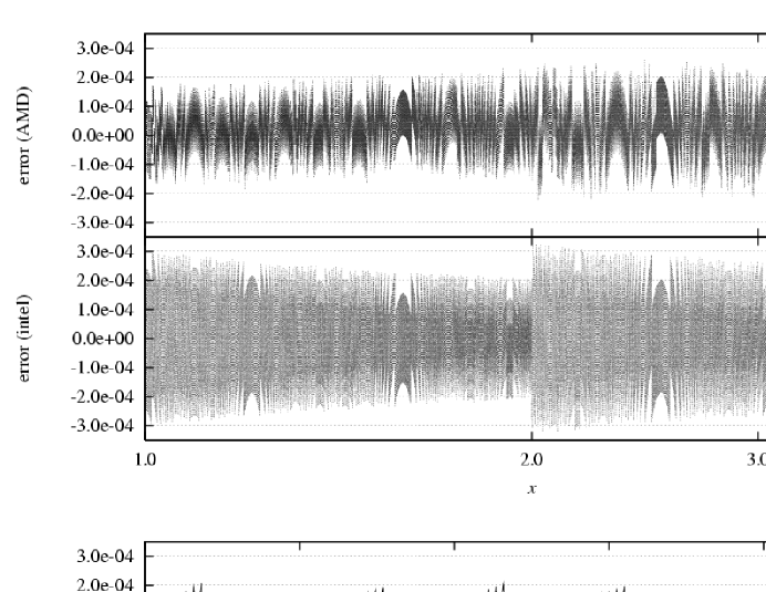
Figure 3: Relative error of the return value of RSQRTSS/PS instructions on AMD Athlon 64 and Intel Pentium 4 for $1\leq x\leq$ 16 (upper) and $1.5\leq x\leq 1.55$ (lower). The errors is periodic for powers of 4.

Note that the actual value returned by this RSQRTSS/PS instruction is implementation dependent. In particular, the AMD Athlon 64 processors and the Intel Pentium 4 processors return different values. Figure 3 shows the errors of the return values as a function of the input values. The AMD implementation has smaller average errors, but at the same time they show a relatively large systematic bias. Even after one Newton-Raphson iteration in double precision, results from both implementations show relatively large biases. Table 3 presents the root mean square error, max error, and bias (mean error) of the approximate value $1/\sqrt{x}$, on a Intel Pentium 4 and an AMD Athlon 64 before/after one Newton-Raphson iteration. Here the error is measured as $1/2(x[\textrm{rsqrt}(x)]^{2}-1)$, and the weight is $1/\textrm{frac}(x)$, where $\textrm{frac}(x)$ is the normalized fraction of the floating-point number $x$. We can correct these biases, at least statistically, by multiplying the resulted force by constants which depend on the processor type used.

Table 3: Errors of approximate inverse square root.

	RMSE	MAX error	Bias
AMD, before N-R	$7.96\times 10^{-5}$	$2.59\times 10^{-4}$	$2.21\times 10^{-5}$
AMD, after N-R	$1.57\times 10^{-8}$	$1.00\times 10^{-7}$	$-9.51\times 10^{-9}$
Intel, before N-R	$1.16\times 10^{-4}$	$3.26\times 10^{-4}$	$-8.37\times 10^{-8}$
Intel, after N-R	$3.05\times 10^{-8}$	$1.60\times 10^{-7}$	$-2.01\times 10^{-8}$
IEEE 754 Single	$3.58\times 10^{-8}$	$8.94\times 10^{-8}$	$1.52\times 10^{-11}$

4.3 Performance

Table 4 shows the performance of four different types of force loops, using SSE2 scalar/vector mode and with/without fast inverse square root.

Table 4: Performance of SSE2 scalar mode and vector mode.

SSE2 mode	scalar		vector
sqrt operation	normal	fast	normal	fast
Cycles per interaction	64.8 cycle	70.5 cycle	69.0 cycle	50.0 cycle
Calculation speed	1.85 Gflops	1.70 Gflops	1.73 Gflops	2.40 Gflops

5 Mixed-precision force loop

As we have summarized in the introduction, SSE2 is the SIMD instruction set for pairs of double-precision words. There are also SSE instructions that work on quadruples of single-precision words. Thus, using the SSE instruction set, we can in principle double the performance. If we perform the initial subtraction between positions and final accumulation of acceleration and potential in double-precision, we can use single-precision SSE functions for all other calculations, including subtraction between velocities and accumulation of jerk, and still maintain a pretty high accuracy. The main complexity here is the question of how to make use of four elements of SSE data type, in parallel. The simplest approach is to calculate the forces on four particles, but in that case we need too many variables, which do not all fit into the registers. We need two XMM registers for each element of force in this way. Instead, we have tried to achieve the maximum speed by calculating the forces from two particles on two particles (making a total of four force calculations) in parallel in SSE.

In the following, we present a detailed description of the implementation of this mixed-precision force loop using SSE/SSE2. We use the term $i$ particles for particles which feel the gravitational force, and $j$ particles for particles which exert the force.

5.1 The data structure for $j$ particles

The data structure for the $j$ particles should contain two particles. The code in list 12 achieves this goal by using the data types v2df and v4sf. Note that for velocities we use the single-precision v4sf data type, since we do not need double-precision accuracy for the velocity. We store the data of the two particles (with indices $j$ and $j+1$) as $(j,j+1)$ for position, and s $(j,j,j+1,j+1)$ for velocity and mass.

List 12: The $j$ particle structure.

⬇

1typedef struct{

2 v2df x[3];

3 v4sf v[3];

4 v4sf m;

5 v4sf pad;

6}Jppack; /* 128-byte */

7typedef Jppack * pJppack;

The variable pad is used to make the size of the structure an exact multiple of 64 bytes.

5.2 The data structure for $i$ particles

We use the following local variables to store two $i$ particles (with indices $i_{0}$ and $i_{1}$).

List 13: Two $i$ particles packed into local variables.

⬇

1v2df xi0[3] = {{x[i0][0], x[i0][0]}, {...} , {...}};

2v2df xi1[3] = {{x[i1][0], x[i1][0]}, {...} , {...}};

3v4sf vi[3] = {{v[i0][0], v[i1][0], v[i0][0], v[i1][0]}, {...}, {...}};

Note that xi0 keeps the position of particle $i_{0}$ in a duplicated way (two 64-bit words of v2df data type store the same data). Similarly, xi1 keeps the data for $i_{1}$. In this way, by subtracting x of the $j$ particle variable from x0 or x1, we can calculate the displacement of two $j$ particles from one $i$ particle. The results are then converted to single-precision format using a cvtpd2ps instruction. (See list 14). After unpcklps (an instruction to pack two words into one words, not to unpack) is issued, the contents of x become $\{x_{j}-x_{i0},\ x_{j}-x_{i1},\ x_{j+1}-x_{i0},\ x_{j+1}-x_{i1}\}$.

For the velocity, we store the data in the order of $(i_{0},i_{1},i_{0},i_{1})$, so that a single subtraction operation provides the four displacement vectors of two $j$ particles from two $i$ particles.

List 14: Subtraction between positions.

⬇

1pJppack pj;

2v2df xi0[3], xi1[3];

3

4for(j=0;j<n;j+=2, pj++){

5 v4sf x, y, z, ftmp;

6 x = __builtin_ia32_cvtpd2ps(pj->x[0] - xi0[0]);

7 ftmp = __builtin_ia32_cvtpd2ps(pj->x[0] - xi1[0]);

8 x = __builtin_ia32_unpcklps(x, ftmp);

5.3 Inverse square root and Newton-Raphson iteration

We use the same NR-iteration as in the previous section. Since we do not need the data conversion between single and double precision formats, the code here actually becomes simpler. List 15 gives this part of the code.

List 15: Calculation of inverse square root in v4sf.

⬇

1v4sf r2, rinv;

2

3rinv = __builtin_ia32_rsqrtps(r2);

4r2 *= rinv; /* start Newton-Raphson */

5r2 *= rinv;

6V4SF_OP_SCALAR(r2, -= , 3.0f);

7rinv *= r2; /* now, rinv = -2.0/r */

5.4 Accumulating acceleration and potential

Before accumulation of acceleration and potential, we now have to convert single-precision data back to double precision. Before doing so, we need to split one piece of 128-bit data with 4 single-precision words into two (effectively) 64-bit words with two single-precision words. This is done by the movhlps instruction. Then we convert the result to double precision using a cvtps2pd instruction. The code appears in list 16.

List 16: Accumulating x element of acceleration.

⬇

1v4sf x, rinv3, ftmp;

2v2df ax;

3

4x *= rinv3;

5ftmp = __builtin_ia32_movhlps(ftmp, x);

6ax += __builtin_ia32_cvtps2pd(x);

7ax += __builtin_ia32_cvtps2pd(ftmp);

For the jerk, we directly accumulate them in quadruples of single-precision words, since we do not need double-precision accuracy for jerk. After total force is obtained, we add up higher two words and lower two words of the accumulated data.

5.5 The whole code

List LABEL:list:mixed shows the entire code. We provide a simple library which one can call to use this function in a way similar to the way the GRAPE hardware is used. We show an example $N$-body code using this library in Appendix 8. Note that actual code in list LABEL:list:mixed is slightly different from code in list (12-16). We use arrays instead of vector types in the $j$ particle structure. Codes in list 14 and 16 are abstracted into macros for readability and saving of registers.

⬇

1 Total code of mixed precision force calculation.

2}, label={list:mixed}]

3static v4sf frv_coeff = {0.75, 0.75, 0.75, 0.75};

4static v2df PotCorrect = {-0.5, -0.5};

5static v2df AccCorrect = {-0.125, -0.125};

6static v4sf V4sfEps2 = {1./65536., 1./65536., 1./65536., 1./65536.};

7static v2df EpsInv = {256.0, 256.0};

8static int Nbody;

9static pJppack Jptr;

10

11void SSEGRAV_Initialize(int nbody, double eps2){

12 double bias = rsqrt_bias(frsqrt_1NR); /* measure bias */

13 double epsinv = 1.0/sqrt(eps2);

14

15 V2DF_OP_SCALAR(PotCorrect, =, -0.5*(1.0-bias));

16 V2DF_OP_SCALAR(AccCorrect, =, -0.125*(1.0 - 3.0*bias));

17 Eps2 = eps2;

18 V2DF_OP_SCALAR(V2dfEps2, =, eps2);

19 V4SF_OP_SCALAR(V4sfEps2, = , (float)eps2);

20 V2DF_OP_SCALAR(EpsInv, =, epsinv);

21 V4SF_OP_SCALAR(frv_coeff, =, 0.75*(1.0 - 2*bias));

22 Nbody = nbody;

23 Jptr = memalign(64, ((1+nbody)/2) * sizeof(Jppack));

24}

25

26#define SUB_PACK(fx, ptr, xi0, xi1, ftmp){ \

27 fx = __builtin_ia32_cvtpd2ps(*(v2df*)(ptr) - xi0); \

28 ftmp = __builtin_ia32_cvtpd2ps(*(v2df*)(ptr) - xi1); \

29 fx = __builtin_ia32_unpcklps(fx, ftmp); \

30}

31

32#define ACCUMLATE(phi, op, fx, ftmp){ \

33 ftmp = __builtin_ia32_movhlps(ftmp, fx); \

34 phi op __builtin_ia32_cvtps2pd(fx); \

35 phi op __builtin_ia32_cvtps2pd(ftmp); \

36}

37

38static inline v2df hadd_ps2pd(v4sf x){

39 v4sf tmp = __builtin_ia32_movhlps(tmp, x);

40 return __builtin_ia32_cvtps2pd(x) + __builtin_ia32_cvtps2pd(tmp);

41}

42

43void SSEGRAV_CalcAccJerkPot(pAccJerk ajout, int *index){

44 int j, k;

45 int nj = Nbody;

46 v2df ax, ay, az, pot;

47 v4sf jx, jy, jz;

48 pJppack pr = Jptr, prj = Jptr;

49 int i0 = index[0], i1 = index[1];

50 static v2df zero = {0.0, 0.0};

51 static v4sf fzero = {0.0, 0.0, 0.0, 0.0};

52 v2df xi0[3], xi1[3];

53 v4sf vi[3];

54 v4sf feps2 = V4sfEps2;

55

56 pot = ax = ay = az = zero;

57 jx = jy = jz = fzero;

58

59 /* set i-particle */

60 for(k=0;k<3;k++){

61 float vi0 = pr[i0/2].v[k][2*(i0%2)];

62 float vi1 = pr[i1/2].v[k][2*(i1%2)];

63

64 V2DF_OP_SCALAR(xi0[k], =, pr[i0/2].x[k][(i0%2)]);

65 V2DF_OP_SCALAR(xi1[k], =, pr[i1/2].x[k][(i1%2)]);

66 V4SF_OP_VECTOR(vi[k], =, vi0, vi1, vi0, vi1);

67 }

68

69 /* force loop */

70 for(j=0;j<nj;j+=2,prj++){

71 v4sf x,y,z,vx,vy,vz;

72 v4sf r2, rv, rinv, rinv2, rinv3;

73

74 __builtin_prefetch(prj+2, 0, 3);

75 __builtin_prefetch(8+(double *)(prj+2), 0, 3);

76

77 SUB_PACK(x, prj->x[0], xi0[0], xi1[0], vx);

78 SUB_PACK(y, prj->x[1], xi0[1], xi1[1], vy);

79 SUB_PACK(z, prj->x[2], xi0[2], xi1[2], vz);

80

81 vx = *(v4sf*)(prj->v[0]) - vi[0];

82 vy = *(v4sf*)(prj->v[1]) - vi[1];

83 vz = *(v4sf*)(prj->v[2]) - vi[2];

84

85 r2 = x*x + y*y + z*z + feps2;

86 rv = vx*x + vy*y + vz*z;

87

88 rinv = __builtin_ia32_rsqrtps(r2);

89 r2 *= rinv;

90 r2 *= rinv;

91 V4SF_OP_SCALAR(r2, -= , 3.0);

92 rinv *= r2;

93

94 rinv2 = rinv * rinv;

95 rv *= frv_coeff; /* 3/4(1-2bias) */

96 rv *= rinv2;

97 rinv *= *(v4sf *)(prj->m);

98

99 rinv3 = rinv * rinv2;

100

101 vx *= rinv3; jx += vx;

102 vy *= rinv3; jy += vy;

103 vz *= rinv3; jz += vz;

104

105 ACCUMLATE(pot, -=, rinv, vx);

106 x *= rinv3;

107 y *= rinv3;

108 z *= rinv3;

109 ACCUMLATE(ax, +=, x, vx);

110 ACCUMLATE(ay, +=, y, vy);

111 ACCUMLATE(az, +=, z, vz);

112

113 x *= rv; jx -= x;

114 y *= rv; jy -= y;

115 z *= rv; jz -= z;

116 }

117

118 /* post loop procedure */

119 pot *= PotCorrect; /* -1/2(1-bias) */

120 {

121 v2df mass = {pr[i0/2].m[2*(i0%2)], pr[i1/2].m[2*(i1%2)]};

122 pot += mass * EpsInv; /* phi_i += m_i/eps */

123 }

124 ax *= AccCorrect; /* -1/8(1-3bias) */

125 ay *= AccCorrect;

126 az *= AccCorrect;

127 {

128 v2df djx, djy, djz;

129 djx = hadd_ps2pd(jx) * AccCorrect;

130 djy = hadd_ps2pd(jy) * AccCorrect;

131 djz = hadd_ps2pd(jz) * AccCorrect;

132

133 V2DF_SCATTER(ax, ajout[0].a, ajout[1].a);

134 V2DF_SCATTER(ay, ajout[0].a+1, ajout[1].a+1);

135 V2DF_SCATTER(az, ajout[0].a+2, ajout[1].a+2);

136 V2DF_SCATTER(djx, ajout[0].j, ajout[1].j);

137 V2DF_SCATTER(djy, ajout[0].j+1, ajout[1].j+1);

138 V2DF_SCATTER(djz, ajout[0].j+2, ajout[1].j+2);

139 V2DF_SCATTER(pot, &ajout[0].pot, &ajout[1].pot);

140 }

141}

5.6 Performance

Table 5: Performance of list LABEL:list:mixed in cycles-per-interaction and Gflops, on Athlon 64 3000+ 2.0GHz, when $N=1024$. The first column is performance of the output by GCC 3.3.1 with option -O3, the second is that of hand-tuned assembly code after GCC.

GCC	Hand-tuning
30.6 cycles	29.6 cycles
3.92 Gflops	4.05 Gflops

Table 5 gives the performance of the code listed above. The second column gives the performance of the code after hand-tuning the assembly output.

The best performance we have measured is 4.05 Gflops, or 3.19 times faster than the original C code described in section 2.

6 Discussion and Summary

In this paper we describe in detail various ways of improving the performance of the force-calculation loop for gravitational interactions between particles. Since modern microprocessors have many instructions which cannot be easily exploited by existing compilers, we can achieve quite a significant performance improvement if we write a few small library in assembly language and/or using instruction-set specific extensions for the compiler offered to us.

Our implementation will give a significant speedup for almost any $N$-body integration program. In addition, we believe that similar optimization is possible in many other compute-intensive applications, within astrophysics as well as in other areas of physics and science in general.

The source code and documentation are available at:
http://grape.astron.s.u-tokyo.ac.jp/~nitadori/phantom/

7 Acknowledgment

We thank Jumpei Niwa for making his Opteron machines available for the development of the optimized force loop and also for his helpful advice. We are also grateful to Eiichiro Kokubo and Toshiyuki Fukushige for their encouragement during the development of the code. We would like to thank all of those who have been involved in the GRAPE project, which has given us a lot of hints for speeding-up of the gravity calculation. P.H. thanks Prof. Ninomiya for his kind hospitality at the Yukawa Institute at Kyoto University, through the Grants-in-Aid for Scientific Research on Priority Areas, number 763, ”Dynamics of Strings and Fields”, from the Ministry of Education, Culture, Sports, Science and Technology, Japan. This research is partially supported by the Special Coordination Fund for Promoting Science and Technology (GRAPE-DR project), also from the Ministry of Education, Culture, Sports, Science and Technology, Japan.

8 Sample $N$-body code using Hermite hierarchical time step scheme

We show sample $N$-body code using Hermite hierarchical time step scheme and the library in subsection 5.5.

⬇

1#include <stdio.h>

2#include <stdlib.h>

3#include <malloc.h>

4

5#define PREFETCH(addr) __builtin_prefetch(addr, 0, 3);

6#define PREFETCHW(addr) __builtin_prefetch(addr, 1, 3);

7#define MEGAHELTZ 2000

8

9struct AccJerk{

10 double a[3];

11 double j[3];

12 double pot;

13};

14

15struct Particle{

16 double x[3];

17 double v[3];

18 double a[3];

19 double j[3];

20 double m;

21 double pot;

22 double time;

23 double timestep;

24}; /* 128-byte */

25

26void CalcAccJerkUsing_iIndex

27(int nbody, int *iIndex, int iNum, struct AccJerk *ajout) {

28 int NumPipe = 2;

29 int iNumRest = iNum;

30

31 while(iNumRest){

32 int ni = MIN(NumPipe, iNumRest);

33 if(ni == 1) iIndex[1] = iIndex[0];

34

35 SSEGRAV_CalcAccJerkPot(ajout, iIndex, nbody);

36

37 iNumRest -= ni;

38 iIndex += ni;

39 ajout += ni;

40 }

41}

42

43int GravityDriver(char *parmfile){

44 int i, k;

45 int nbody;

46 double epsinv, TimeEnd, dEOutTime, MaxStep, Eta_s, SqrtEta;

47 double SystemTime = 0.0;

48 double eps2;

49 double InitEnergy;

50 FILE *fpin = NULL, *fpout = NULL;

51 struct Particle *ptcl;

52 struct AccJerk *ajnew;

53 int *iIndex;

54 long NumPtclStep = 0, NumStep = 0;

55 long tsc0, tsc1;

56 double cycle;

57 long CyclePredict = 0, CycleForce = 0

58 CycleCorrect = 0, CycleTot = 0;

59 double WallTime;

60

61 GetParam(parmfile, &epsinv, &TimeEnd, &MaxStep,

62 &dEOutTime, &Eta_s, &SqrtEta, &fpin, &fpout);

63 if(epsinv == 0.) eps2 = 0.;

64 else eps2 = 1.0/(epsinv*epsinv);

65

66 assert(fpin != NULL);

67 assert(1 == fscanf(fpin,"%d\n", &nbody));

68 printf("N␣=␣%d\n", nbody);

69

70 ptcl = memalign(64, nbody * sizeof(struct Particle));

71 ajnew = memalign(64, (1+nbody) * sizeof(struct AccJerk));

72 iIndex = calloc(1+nbody , sizeof(int));

73

74 ReadSnapshot(fpin, nbody, ptcl, &SystemTime);

75

76 SSEGRAV_Initialize(nbody, eps2/*, epsinv*/);

77 BSTEP_Initialize(nbody, 0.0, MaxStep);

78

79 SSEGRAV_Predict(ptcl, SystemTime/*, nbody*/);

80

81 /* initial step */

82 for(i=0;i<nbody;i++) iIndex[i] = i;

83 rdtscll(tsc0);

84 CalcAccJerkUsing_iIndex(nbody, iIndex, nbody, ajnew);

85 rdtscll(tsc1);

86 cycle = (tsc1 - tsc0) / ((double)nbody * nbody);

87 printf("%f␣cycle␣per␣interruction,␣%F␣Gflops\n\n",

88 cycle, MEGAHELTZ/1.e3/cycle*60.0);

89

90 for(i=0;i<nbody;i++){

91 for(k=0;k<3;k++){

92 ptcl[i].a[k] = ajnew[i].a[k];

93 ptcl[i].j[k] = ajnew[i].j[k];

94 }

95 ptcl[i].pot = ajnew[i].pot;

96 InitTimestep(ptcl+i, Eta_s, MaxStep);

97 BSTEP_PushAParticle(i, ptcl[i].timestep, &ptcl[i].timestep);

98 }

99 InitEnergy = GetEnergy(ptcl, nbody);

100 PrintEnegy(ptcl, nbody, InitEnergy, SystemTime);

101

102 /* evolve */

103 rdtscll(tsc0);

104 CycleTot -= tsc0;

105 CycleCorrect -= tsc0;

106 while(1){

107 int iNum;

108

109 BSTEP_PullParticles(iIndex, &iNum, &SystemTime);

110 rdtscll(tsc0);

111 CycleCorrect += tsc0;

112 if(SystemTime >= TimeEnd) break;

113

114 CyclePredict -= tsc0;

115 SSEGRAV_Predict(ptcl, SystemTime/*, nbody*/);

116 rdtscll(tsc0);

117 CyclePredict += tsc0;

118

119 CycleForce -= tsc0;

120 CalcAccJerkUsing_iIndex(nbody, iIndex, iNum, ajnew);

121 rdtscll(tsc0);

122 CycleForce += tsc0;

123

124 CycleCorrect -= tsc0;

125 for(k=0;k<iNum;k++){

126 int ii = iIndex[k];

127 char *addr = (char *)(ptcl + iIndex[k+1]);

128 PREFETCHW(addr);

129 PREFETCHW(addr+64);

130 PREFETCH(ajnew+k+1);

131 HermiteCorrect(ptcl+ii, ajnew+k, SqrtEta);

132 BSTEP_PushAParticle

133 (ii, ptcl[ii].timestep, &ptcl[ii].timestep);

134 }

135 if(fmod(SystemTime, dEOutTime) == 0.0){

136 for(i=0;i<nbody;i++) ptcl[i].pot = ajnew[i].pot;

137 PrintEnegy(ptcl, nbody, InitEnergy, SystemTime);

138 }

139 NumPtclStep += iNum;

140 NumStep++;

141 }

142 rdtscll(tsc1);

143 CycleTot += tsc1;

144

145 WallTime = (double)CycleTot/MEGAHELTZ / 1.E6;

146 printf("Wall␣clock␣time:␣%f␣sec\n", WallTime);

147 printf("predict:␣%f␣usec/blockstep,␣%f␣cycle/loop\n",

148 (double)CyclePredict/NumStep/MEGAHELTZ,

149 (double)CyclePredict/(NumStep*nbody));

150 printf("force␣␣:␣%f␣usec/blockstep,␣%f␣cycle/loop\n",

151 (double)CycleForce/NumStep/MEGAHELTZ,

152 (double)CycleForce/(NumPtclStep*nbody));

153 printf("correct:␣%f␣usec/blockstep,␣%f␣cycle/loop\n",

154 (double)CycleCorrect/NumStep/MEGAHELTZ,

155 (double)CycleCorrect/(NumPtclStep));

156 printf("%f␣particles/blockstep\n\n", (double)NumPtclStep/NumStep);

157

158 /* final synchronizing step */

159 SSEGRAV_Predict(ptcl, TimeEnd/*, nbody*/);

160 for(i=0;i<nbody;i++) iIndex[i] = i;

161 CalcAccJerkUsing_iIndex(nbody, iIndex, nbody, ajnew);

162 for(i=0;i<nbody;i++){

163 ptcl[i].pot = ajnew[i].pot;

164 ptcl[i].timestep = TimeEnd - ptcl[i].time;

165 HermiteCorrect(ptcl+i, ajnew+i, SqrtEta);

166 }

167 PrintEnegy(ptcl, nbody, InitEnergy, TimeEnd);

168

169 if(fpout) WriteSnapshot(fpout, nbody, ptcl, TimeEnd);

170

171 SSEGRAV_Finalize();

172 BSTEP_Finalize();

173 free(ptcl);

174 free(ajnew);

175 free(iIndex);

176

177 fclose(fpin);

178 fclose(fpout);

179 return 0;

180}

181

182int main(){

183 GravityDriver("initparm");

184 return 0;

185}

References

- (1)
- Barnes and Hut (1986) Barnes, J. & Hut, P. 1986, Nature, 324, 446
- Karp (1993) Karp, A. H. 1993, Scientific Programming, 1, 133
- Makino & Aarseth (1992) Makino, J. & Aarseth, S. J. 1992, PASJ, 44, 141
- Makino et al. (2001) Makino, J. & Fukushige, T. 2001, In The SC2001 Proceedings, CD–ROM. Los Alamitos, IEEE Comp. Soc.
- Makino et al. (2003) Makino, J., Fukushige, T., Koga, M., & Namura, K. 2003, PASJ, 55, 1163
- Sugimoto et al. (1990) Sugimoto, D., Chikada, Y., Makino, J., Ito, T., Ebisuzaki, T., & Umemura, M. 1990, Nature, 345, 33.
- Warren et al. (1997) Warren, M. S., Salmon, J. K.,Becker, D. J., Goda, M. P., & Sterling, T. 1997, In The SC97 Proceedings, CD–ROM. IEEE, Los Alamitos, CA.
- Intel (2004) Intel 2004, IA-32 Intel Architecture Optimization Reference Manual
- AMD (2004) AMD 2004, Software Optimization Guide for AMD Athlon 64 and AMD Opteron Processors
- GCC (2005) GCC 2005, Using the GNU Compiler Collection, http://gcc.gnu.org/onlinedocs/