Infall and Outflow around the HH 212 protostellar system

Abstract

HH 212 is a highly collimated jet discovered in H₂ powered by a young Class 0 source, IRAS 05413-0104, in the L1630 cloud of Orion. We have mapped around it in 1.33 mm continuum, ¹²CO ($J=2-1$), ¹³CO ($J=2-1$), C¹⁸O ($J=2-1$), and SO ($J_{K}=6_{5}-5_{4}$) emission at $\sim$ $2.5^{\prime\prime}$ resolution with the Submillimeter Array. A dust core is seen in the continuum around the source. A flattened envelope is seen in C¹⁸O around the source in the equator perpendicular to the jet axis, with its inner part seen in ¹³CO. The structure and kinematics of the envelope can be roughly reproduced by a simple edge-on disk model with both infall and rotation. In this model, the density of the disk is assumed to have a power-law index of $p=-1.5$ or $-2$, as found in other low-mass envelopes. The envelope seems dynamically infalling toward the source with slow rotation because the kinematics is found to be roughly consistent with a free fall toward the source plus a rotation of a constant specific angular momentum. A ¹²CO outflow is seen surrounding the H₂ jet, with a narrow waist around the source. Jetlike structures are also seen in ¹²CO near the source aligned with the H₂ jet at high velocities. The morphological relationship between the H₂ jet and the ¹²CO outflow, and the kinematics of the ¹²CO outflow along the jet axis are both consistent with those seen in a jet-driven bow shock model. SO emission is seen around the source and the H₂ knotty shocks in the south, tracing shocked emission around them.

1 Introduction

Despite recent progress, the detailed physical processes in the early stages of low-mass star formation are still uncertain. Currently, the most detailed and successful model of low-mass star formation is the four-stage model proposed in the late 80’s by Shu, Adams, & Lizano (1987). In the first stage, slowly rotating molecular cloud cores form within a molecular cloud as magnetic and turbulent support is lost through ambipolar diffusion. In the second stage, a molecular cloud core becomes dynamically unstable and collapses from the inside-out, forming a protostar surrounded by an accretion disk deeply embedded within an infalling envelope of dust and gas. In the third stage, as the protostar continues accreting mass through the accretion disk, a stellar wind breaks out along the rotational axis of the system, creating a bipolar outflow. In the fourth stage, the infall and accretion terminate, leaving a newly formed star surrounded by a circumstellar disk. In this paper, we investigate the protostellar collapse and outflow in the second and third stages, with the Submillimeter Array (SMA) observations around a young protostar, IRAS 05413-0104, and its remarkable jet HH 212.

IRAS 05413-0104 is a cold, low-luminosity ($\sim$ 14 $L_{\odot}$), low-mass source (Zinnecker et al., 1992), located at a distance of 460 pc in the L1630 cloud of Orion. It is surrounded by a cold ($\sim$ 14 K), flattened (with an aspect ratio of 2:1) rotating NH₃ envelope with a diameter of 12,000 AU (Wiseman et al., 2001). It is detected also at 1.1 mm (Zinnecker et al., 1992) and 1.3 mm (Chini et al., 1997), with a high ratio of millimeter-wave luminosity to bolometric luminosity. It is thus classified as a Class 0 source, which has much material to be accreted still from the surrounding molecular gas envelope (Andre et al., 2000).

HH 212 is a remarkable jet with a length of $\sim$ 240 arcsecs ($\sim$ 0.6 pc) powered by the IRAS source. It was discovered in the rotational-vibrational $v=1-0$ S(1) emission line of H₂ at $\lambda=2.122$ $\mu$m (Zinnecker, McCaughrean, & Rayner, 1998). It is highly collimated and symmetric with matched pairs of shock knots (knotty shocks) and bow shocks on either side of the IRAS source. Strong water masers are seen moving at $\sim$ 60 km s^-1 along the jet axis near the IRAS source (Claussen et al., 1998). Shocked SiO emission is seen along the jet axis (Chapman et al., 2002) and around the source (Gibb et al., 2004). CO outflow is also seen surrounding the H₂ jet (Lee et al., 2000). Deep observations in H₂ with the ESO Very Large Telescope (VLT) show a pair of diffuse nebulae near the bases of the jet, probably tracing the outflow cavity walls illuminated by the bright knotty shocks around the source (McCaughrean et al., 2002). Based on the relative magnitude of the proper motions and radial velocities of the water masers, the CO outflow is believed to lie within 5^∘ of the plane of the sky (Claussen et al., 1998), and is thus an excellent system to investigate the transverse kinematics of outflow.

Here, we study in detail the circumstellar envelope around the IRAS source, the molecular outflow surrounding the H₂ jet, and the interaction between them, with the SMA observations in 1.33 mm continuum, ¹²CO ($J=2-1$), ¹³CO ($J=2-1$), C¹⁸O ($J=2-1$), and SO ($J_{K}=6_{5}-5_{4}$) emission at high angular and velocity resolutions. It is currently believed that 1.33 mm continuum mainly traces dust core, ¹²CO (particularly in interferometric observations) mainly traces molecular outflow, C¹⁸O mainly traces envelope, ¹³CO traces both molecular outflow and envelope, and SO traces mainly shock interactions.

2 Observations

Observations in 1.33 mm continuum, ¹²CO ($J=2-1$), ¹³CO ($J=2-1$), C¹⁸O ($J=2-1$), and SO ($J_{K}=6_{5}-5_{4}$) emission toward the IRAS source and the H₂ jet were made between 2004 November and 2005 March on top of Mauna Kea with the SMA in the compact configuration (see Table 1). Seven antennas were used in the array, giving baselines with projected lengths ranging from 14.1 to 136 m, resulting in a synthesized beam (with natural weighting) with a size of $2.8^{\prime\prime}$$\times$$2.4^{\prime\prime}$ at 230 GHz. With a shortest projected baseline of 14.1 m, our observations were insensitive to structures more extended than $15^{\prime\prime}$ ($\sim$ 7000 AU) at the 10% level. The FWHP of the primary beam is $55^{\prime\prime}$, and 9 pointings were used to map the whole jet system. The digital correlator was set up with a bandwidth of 104 MHz for each band (or chunk). We used 512 spectral channels for ¹²CO, C¹⁸O, and ¹³CO and 256 spectral channels for SO, resulting in a velocity resolution per channel of $\sim$ 0.27 km s^-1 for ¹²CO, C¹⁸O, and ¹³CO, and 0.55 km s^-1 for SO. The 1.33 mm (or 225 GHz) continuum emission was also recorded with a total bandwidth of $\sim$ 4 GHz. In our observation, a phase calibrator (Quasar 0423-013) was observed every 20 minutes to calibrate the phases of the source. A planet (Uranus) was observed to calibrate the fluxes. The data were calibrated with the MIR package adapted for the SMA. The calibrated data were processed with the MIRIAD package. The dirty maps that were produced from the calibrated data and corrected for the primary beam attenuation were deconvolved using the Steer clean method. The final channel maps were obtained by convolving the deconvolved maps with a synthesized (Gaussian) beam fitted to the main lobe of the dirty beam. The velocities of the channel maps are LSR.

3 Results

In the following, the IRAS source is assumed to have a refined position at $\alpha_{(2000)}=05^{\mathrm{h}}43^{\mathrm{m}}51^{\mathrm{s}}_{{}^{.}}408$, $\delta_{(2000)}=-01\arcdeg 02\arcmin 53.13\arcsec$, which was found at $\lambda=3.5$ cm with the VLA at an angular resolution of $0.3^{\prime\prime}$ (Galván-Madrid et al., 2004). The systemic velocity in this region was assumed to be 1.8 km s^-1 in CO J=1-0 observations (Lee et al., 2000) and 1.6 km s^-1 in NH₃ observations (Wiseman et al., 2001). Here, it is assumed to be $1.7\pm 0.1$ km s^-1. Throughout this paper, the observed velocity is the velocity with respect to this systemic velocity. For comparison, our observations are always plotted with the H₂ image of the jet recently obtained with the VLT (McCaughrean et al., 2002). The axis of the H₂ jet has a position angle of $\sim$ 23^∘. The H₂ jet is almost in the plane of the sky, with the blueshifted side to the north and the redshifted side to the south of the source.

3.1 1.33 mm Continuum Emission

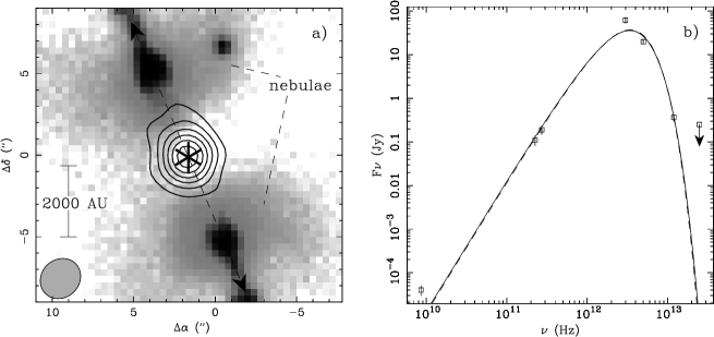
Figure 1: (a) 1.33 mm continuum contours plotted on top of the H₂ image adopted from McCaughrean et al. (2002). The contours go from 3 to 18 $\sigma$ with a step of 3 $\sigma$, where $\sigma=3.5$ mJy beam^-1. The asterisk indicates the IRAS source. Note that the (0, 0) position here corresponds to $\alpha_{(2000)}=05^{\mathrm{h}}43^{\mathrm{m}}51^{\mathrm{s}}_{{}^{.}}30$, $\delta_{(2000)}=-01\arcdeg 02\arcmin 53.0\arcsec$. (b) Simple fits to the SED of the continuum source with $\Omega=1.2$ (solid line) and 2.3 (dashed line) arcsec².

Continuum emission is detected around the source at $\lambda=1.33$ mm with a flux of 0.11$\pm 0.03$ Jy in between the diffuse nebulae seen in H₂ (Fig. 1). This flux is similar to the peak flux in an $11^{\prime\prime}$ beam around the source found by Chini et al. (1997) with the IRAM 30 telescope. The emission is not resolved and shows a slight elongation along the jet axis. Previously, continuum emission has been detected around the source at $\lambda=1.1$ mm by the JCMT with a flux of 0.19 Jy (Zinnecker et al., 1992). Continuum emission has also been detected in the infrared by the IRAS. The fluxes corrected for extinction are 0.37, 19.9, and 61.9 Jy at $\lambda=25$, 60, and 100 $\mu$m, respectively. It was not detected at $\lambda=12$ $\mu$m. The spectral energy distribution (SED, see Fig. 1b) is consistent with a Class 0 source. It clearly suggests that the continuum emission at $\lambda=1.33$ mm is thermal emission from a dust core around the source.

The temperature of the dust core can be derived from the SED. For simplicity, we assume a constant temperature for the dust core, and the solid angle subtended by the dust core, $\Omega$, is independent of frequency, $\nu$, so that the observed flux is given by

$$F_{\nu}=\Omega(1-e^{-\tau_{\nu}})B_{\nu}(T_{dust})$$ (1)

where the optical depth

$$\tau_{\nu}=\kappa_{\nu}\sigma$$ (2)

with $\kappa_{\nu}$ being the mass opacity and $\sigma$ being the column density. With (see, e.g., Beckwith et al., 1990)

$$\kappa_{\nu}=0.1(\frac{\nu}{10^{12}\;\textrm{Hz}})^{\beta}\;\textrm{cm}^{2}\;\textrm{g}^{-1}$$ (3)

the optical depth can be simplified as

$$\tau_{\nu}=(\nu/\nu_{o})^{\beta}$$ (4)

with an optical depth of unity at $\nu_{o}$. As can be seen from the SED, the emission are optically thin at $\lambda=1.1$ and 1.33 mm, and their flux ratio implies that $\beta\sim 1$. The solid angle $\Omega$ is uncertain, likely $<2.3\arcsec\times 1\arcsec$ (see Fig. 1a). With $\Omega=1.2$ and 2.3 arcsec², the SED can be fitted with $T_{dust}=47.6$ K and $\nu_{o}=3\times 10^{12}$ Hz, and $T_{dust}=45.4$ K and $\nu_{o}=6\times 10^{12}$ Hz, respectively (see Fig. 1b). Thus, $T_{dust}$ is assumed to be 46 K. With this temperature and the optically thin emission at $\lambda=1.33$ mm, the (gas $+$ dust) mass is estimated to be

$$M\sim\frac{D^{2}F_{\nu}}{B_{\nu}(T_{dust})\kappa_{\nu}}\sim 0.08M_{\odot}$$ (5)

where the distance to the source $D=460$ pc.

3.2 C¹⁸O ($J=2-1$) emission

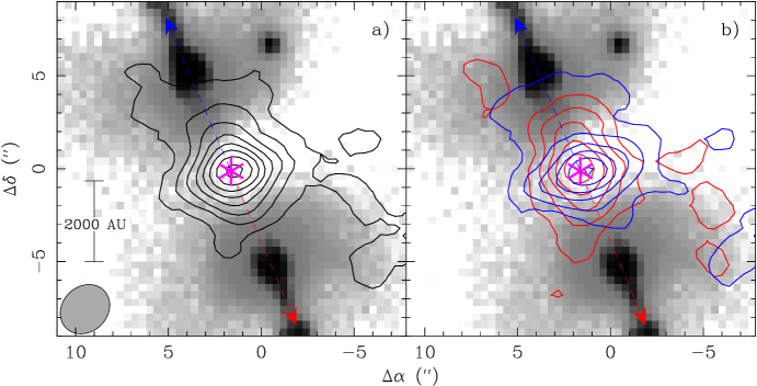
Figure 2: C¹⁸O emission plotted on top of the H₂ image, with the asterisk indicating the IRAS source. (a) Total emission integrated over 2.2 km s^-1 from $-$1.1 km s^-1 to 1.1 km s^-1. The contours go from 2 to 23 $\sigma$ with a step of 3 $\sigma$, where $\sigma=0.11$ Jy beam^-1. (b) Redshifted (red contours) and blueshifted (blue contours) emission, integrated over 1.1 km s^-1 on the redshifted and blueshifted side, respectively. The contours go from 2 to 17 $\sigma$ with a step of 3 $\sigma$, where $\sigma=0.08$ Jy beam^-1 km s^-1.

In C¹⁸O, an envelope is seen around the source in the equator between the diffuse nebulae (Fig. 2a). Faint shells (2 $\sigma$ contours) are also seen opening to the north and south surrounding the bases of the nebulae. The envelope is better seen in the blueshifted emission, in which the shells are much fainter than the envelope (Fig. 2b). It is extended across the source from the east to the west with a position angle of $\sim 110$^∘$\pm 10$^∘, perpendicular to the jet axis. It is flattened with an (deconvolved) FWHM extent of $\sim$ $4.3^{\prime\prime}$ (or 2000 AU at 460 pc) and an aspect ratio of $\sim$ 3:2. In the redshifted emission, the envelope is less extended. Since the redshifted emission around the bases of the nebulae is as bright as that of the envelope, the redshifted emission appears extended along the jet axis.

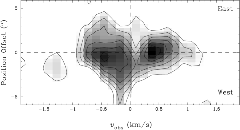
Figure 3: PV diagram of C¹⁸O emission cut along the major axis of the flattened envelope.

A cut along the major axis of the flattened envelope shows a PV structure with the emission seen across the source with the redshifted and blueshifted peaks on either side of the source (Fig. 3). The blueshifted emission spreads across the source with a peak at ($-0.5$ km s^-1, $-$$0.45^{\prime\prime}$) in the west, while the redshifted emission spreads across the source with a peak at (0.35 km s^-1, $0.1^{\prime\prime}$) in the east. This PV structure is similar to that seen in C¹⁸O J=1-0 toward an edge-on dynamically infalling envelope with rotation around a young Class 0 source IRAS 04368+2557 in L1527 (Ohashi et al., 1997). It suggests that the material of the flattened envelope is also infalling toward the source with rotation, with the redshifted emission from the nearside, while the blueshifted emission from the farside.

3.3 ¹³CO ($J=2-1$) emission

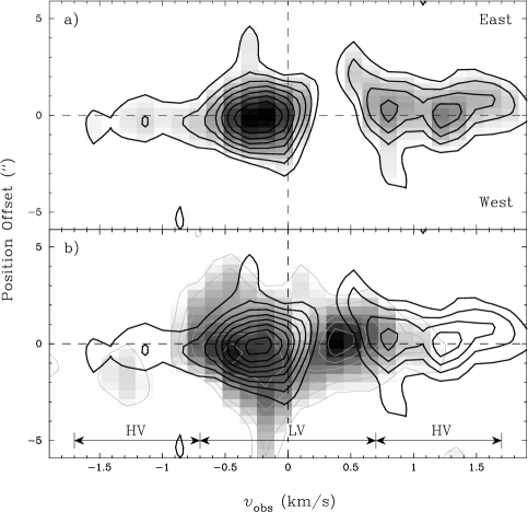
Figure 5: PV diagrams of C¹⁸O and ¹³CO emission cut along the major axis of the flattened envelope. (a) for ¹³CO. (b) Overlay of the two. Here, LV denotes low velocity and HV denotes high velocity.

In ¹³CO, the emission peaks at the source and extends to the bases of the nebulae (Fig. 4a). The emission can be decomposed into low-velocity and high-velocity components (see Fig. 5b and the explanation in the following paragraph). At low velocity, the emission forms a hourglass structure with a narrow waist around the source (Fig. 4b), with the blueshifted emission opening to the north and the redshifted emission opening to the south around the bases of the nebulae (Fig. 4c). Around the source, the blueshifted emission peaks a little to the west, while the redshifted emission shifts to the east of the source and is weak along the major axis of the flattened C¹⁸O envelope. At high velocity, the blueshifted emission peaks to the west while the redshifted emission peaks to the east of the source (Fig. 4d). The emission also extends to the north and south along the jet axis.

A cut across the ¹³CO waist along the major axis of the flattened C¹⁸O envelope shows that the ¹³CO emission has a larger velocity range than that of the C¹⁸O emission (Figs. 5a and 5b). The velocity range is thus decomposed into low-velocity and high-velocity components, with the range of the low-velocity component similar to that of the C¹⁸O emission. At low velocity, the blueshifted emission is seen across the source along the major axis of the flattened envelope with a peak at ($-0.3$ km s^-1, $0.1^{\prime\prime}$), and a redshifted dip is seen around 0.4 km s^-1 across the source along the major axis of the flattened envelope. This dip may be due to the absorption of a cold material infalling toward the source (Evans, 1999), which is probably traced by the bright C¹⁸O emission around that velocity (see Fig. 5b). At high velocity, the redshifted and blueshifted emission are each confined on one side of the source, as seen in Figure 4d. This high-velocity emission is unlikely to be from outflow, with the redshifted and blueshifted emission on either side of the source. This high-velocity emission may trace the inner part of the envelope, where the rotation starts to dominate over the infall motion and a rotationally supported disk starts to form.

3.4 ¹²CO ($J=2-1$) emission

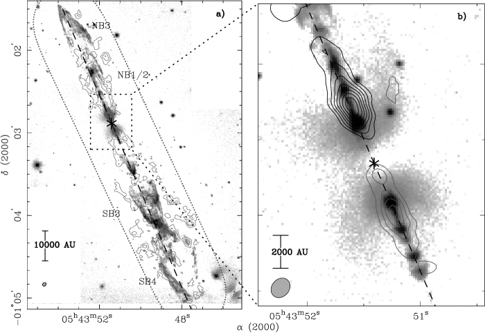
Figure 6: ¹²CO emission plotted on top of the H₂ image adopted from McCaughrean et al. (2002), with the asterisk indicating the IRAS source. The black dotted line outlines the observed region in our observations. (a) Black contours: Total emission integrated over 32 km s^-1 from $-$16 to 16 km s^-1. The contours go from 2 to 24 $\sigma$ with a step of 2 $\sigma$, where $\sigma=0.68$ Jy beam^-1 km s^-1. (b) Black contours: High blueshifted emission integrated from $-$5 to $-$16 km s^-1. The contours go from 3 to 21 $\sigma$ with a step of 3 $\sigma$, where $\sigma=0.42$ Jy beam^-1 km s^-1. Gray contours: High redshifted emission integrated from 2 to 13 km s^-1. The contours go from 3 to 12 $\sigma$ with a step of 3 $\sigma$, where $\sigma=0.42$ Jy beam^-1 km s^-1. Here, the velocity ranges are selected to show the jetlike structures as much as possible, without the confusion from the shell emission.

A ¹²CO outflow is seen surrounding the H₂ jet, with a narrow waist around the source (Fig. 6). Near the source, limb-brightened outflow shells are seen opening to the north and south from the source surrounding the H₂ jet. The shells may extend further down along the jet axis, connecting to the prominent H₂ bow shocks SB4 and NB3, as seen in lower $J$ transition line of ¹²CO (Lee et al., 2000). Deeper observations with shorter baselines are needed to confirm this. At high velocities, the ¹²CO emission is jetlike, i.e., collimated and knotty, much like the H₂ jet, located inside the cavity defined by the diffuse nebulae and ¹²CO outflow shells (Fig. 6b). In the south, ¹²CO outflow shell is seen coincident with the H₂ bow shock SB4, probably tracing the ambient material swept up by the H₂ bow shock. Note that here the ¹²CO outflow shell is mainly seen on one side of the bow shock, which is brighter in H₂.

Assuming an optically thin emission, a temperature of 50 K, and a ¹²CO abundance of 8.5$\times 10^{-5}$ with respect to molecular hydrogen (Frerking et al., 1982), the H₂ column density of the shells around the source and the bow shock SB4 is found to be $\sim 10^{20}$ cm^-2. Assuming that the shell thickness is $\sim$ $3^{\prime\prime}$ (see Fig. 6), the density is $\sim$ 5$\times 10^{3}$ cm^-3. The peak column density along the jet axis is $\sim 5\times 10^{20}$ cm^-2. Assuming that the thickness is $\sim$ $2^{\prime\prime}$, the density is $\sim$ 4$\times 10^{4}$ cm^-3. Note that due to the absorption of the ambient cloud, that part of the emission is optically thick, and that part of the emission is resolved out by the interferometer, the values presented here are lower limits of the true values.

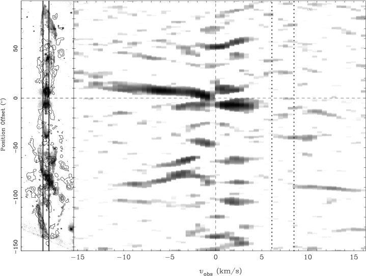
Figure 7: Left: The H₂ jet and CO outflow, with the outflow axis rotated to be aligned with the y-axis, The two vertical lines indicate the width of the cut for the position-velocity diagram. Right: Position-velocity diagram of the CO outflow cut along the outflow axis. The two dotted lines around 7 km s^-1 indicate the velocity range of a foreground ambient cloud seen by the FCRAO single-dish telescope (Lee et al., 2000).

This outflow, which is almost in the plane of the sky, is one of the best candidates to study the outflow kinematics transverse to the jet axis. A cut along the jet axis shows a series of convex spur PV structures on both redshifted and blueshifted sides with the highest velocity near the H₂ bow tips and knots (Fig. 7). Notice that the redshifted emission around $\sim 7$ km s^-1 merges with the foreground ambient cloud emission in velocity and thus is mostly resolved out from our observations. These PV structures are similar to those seen in lower $J$ transition line of ¹²CO (Lee et al., 2000), but with a higher velocity around the H₂ knots and bow tips. These PV structures suggest that the outflow is accelerated by the shocks localized at the H₂ bow tips and knots, so that the velocity of the outflow decreases rapidly away from the tips, similar to that seen in a pulsed jet simulation (see, e.g., Lee et al., 2001).

3.5 SO ($J_{K}=6_{5}-5_{4}$) emission

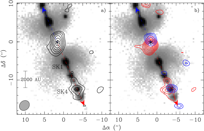
Figure 8: SO emission plotted on top of the H₂ image, with the asterisk indicating the IRAS source. (a) Total emission integrated over 16 km s^-1 from -7 to 9 km s^-1. The contours go from 3 to 13 $\sigma$ with a step of 2 $\sigma$, where $\sigma=0.35$ Jy beam^-1 km s^-1. (b) Redshifted (red contours) and blueshifted (blue contours) emission, integrated from -7 to -2 km s^-1 and from 2 to 9 km s^-1, respectively. The contours go from 3 to 10 $\sigma$ with a step of 1 $\sigma$, where $\sigma=0.23$ Jy beam^-1 km s^-1.

SO emission is detected around the source and the H₂ knots in the south, especially the knot SK4 (Fig. 8a). Around the source, the emission is not well resolved and is slightly elongated with a major axis about mid-way between the jet and envelope axes. The blueshifted emission is to the north, while the redshifted emission is to the south of the source (Fig. 8b), similar to that seen in the H₂ jet, suggesting that the SO emission may arise from interactions with the jet. The peaks of the redshifted and blueshifted emission, however, are a little off the jet axis, with the redshifted one shifted to the east and the blueshifted one shifted to the west, suggesting that the SO emission may also arise from the envelope. Around the knot SK4, the redshifted emission is to the east while the blueshifted emission is to the west, similar to that seen in the flattened C¹⁸O envelope.

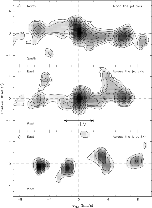
Figure 9: PV diagrams of SO emission. (a) A cut along the jet axis for the emission around the source. (b) A cut across the jet axis for the emission around the source. LV denotes low velocity. (c) A cut across the jet axis for the emission around the knot SK4.

The SO emission around the source may consist of more than one component. A cut along the jet axis shows two peaks at high velocity, one is blueshifted at ($-5.5$ km s^-1, $0.64^{\prime\prime}$) in the north and one is redshifted at (6.1 km s^-1, $-$$0.53^{\prime\prime}$) in the south (Fig. 9a). The rapid increase in the velocity suggests that the SO emission at high velocity indeed arises from shock interactions with the jet. However, the SO emission seen around the systemic velocity may not be produced by the shock interactions, because of its low velocity. A cut across the jet axis shows a rather symmetric PV structure about the source (Fig. 9b) at low velocity. The spatial extent and the velocity distribution (i.e., the redshifted emission is to the east and the blueshifted emission is to the west) of this PV structure are similar to that of the flattened C¹⁸O envelope, suggesting that the SO emission at low velocity may be associated with the flattened envelope. There are also high blueshifted and redshifted emission at $\sim$ $3^{\prime\prime}$ in the east.

A cut across SK4 shows that the redshifted emission is to the east, while the blueshifted emission is to the west (Fig. 9c), as seen in Figure 8b. The velocity extent seems to be similar to that around the source, with the higher velocity near the jet axis.

3.6 Summary

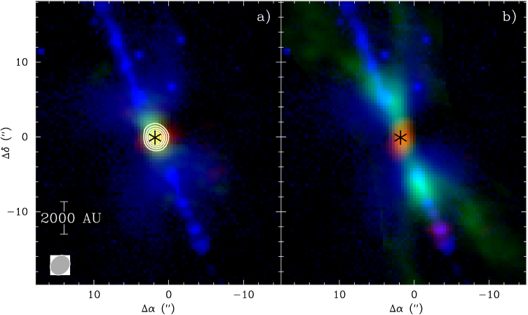
Figure 10: (a) Composite image of continuum (white contours), C¹⁸O (red), ¹³CO (green), and H₂ (blue) emission. (b) Composite image of SO (red), ¹²CO (green), and H₂ (blue) emission.

In this section, we summarize our observations with two composite figures, Figures 10a and 10b. From these figures, it is clear that (1) the dust core seen in continuum and the ¹³CO waist are surrounded by the flattened C¹⁸O envelope in the equator, and thus may both trace the inner part of the envelope; (2) the ¹³CO emission extends to the north and south from the source, surrounding the bases of the nebulae; (3) the ¹²CO outflow appears as limb-brightened shells surrounding the H₂ jet, and (4) the SO emission is detected around the source and the H₂ knots in the south.

4 Modeling of Circumstellar Envelope

In the following, a simple edge-on disk model with both infall and rotation is used to reproduce the structures and kinematics of the flattened C¹⁸O envelope and the ¹³CO waist seen around the source. In this model, the disk is assumed to have a constant thickness of $H$, an inner radius of $R_{\textrm{\scriptsize in}}$, and an outer radius of $R_{\textrm{\scriptsize out}}$. The number density of molecular hydrogen is assumed to be given by (in Cylindrical coordinates)

$$n=n_{\textrm{\scriptsize 0}}(\frac{R}{R_{\textrm{\scriptsize 0}}})^{p}$$ (6)

where $n_{\textrm{\scriptsize 0}}$ is the density at a characteristic radius of $R_{\textrm{\scriptsize 0}}=460$ AU (i.e., $1^{\prime\prime}$) and $p$ is a power-law index. The temperature of the envelope is uncertain and assumed to be given by

$$T=T_{\textrm{\scriptsize 0}}(\frac{R}{R_{\textrm{\scriptsize 0}}})^{q}$$ (7)

where $T_{\textrm{\scriptsize 0}}$ is the temperature at $R_{\textrm{\scriptsize 0}}$ and $q$ is a power-law index. The abundances of C¹⁸O and ¹³CO relative to molecular hydrogen are assumed to be constant and given by $1.7\times 10^{-7}$ and $9.5\times 10^{-7}$, respectively (Frerking et al., 1982).

The detailed radial profiles of the infall velocity and the rotation velocity can not be determined from our observations obtained at current spatial and velocity resolutions. For simplicity, we assume a dynamical infall that results in a free fall for the infall velocity. Assuming that the mass of the envelope is small compared with that of the source, we have

$$v_{R}=\sqrt{\frac{2GM_{*}}{R}}\sim 0.76\sqrt{\frac{M_{*}}{0.15M_{\odot}}\frac{R_{\textrm{\scriptsize 0}}}{R}}\;\;\;\textrm{km s}^{-1}$$ (8)

where $M_{*}$ is the mass of the source. The rotation seems differential with the velocity increasing toward the source (see Figs. 3 and 5). However, the rotation is unlikely to be Keplerian, because the rotation velocity, as found in the following, is much smaller than the infall velocity. In a dynamically infalling envelope with slow rotation, specific angular momentum of each gas element is considered to be conserved, until the infall motion shifts to the centrifugally supported motion around the radius where the rotation velocity is comparable to the infall velocity (see, e.g., Nakamura, 2000). Thus, the rotation velocity is assumed to be given by

$$v_{\phi}=v_{\phi\textrm{\scriptsize 0}}\frac{R_{\textrm{\scriptsize 0}}}{R}$$ (9)

where $v_{\phi\textrm{\scriptsize 0}}$ is the rotation velocity at $R_{\textrm{\scriptsize 0}}$ and it depends on the initial angular momentum at the outer radius. In the model calculations, radiative transfer is used to calculate the emission, with an assumption of local thermal equilibrium. For simplicity, the line width is assumed to be given by the thermal line width only. The line width due to turbulence is not included in our model. The channel maps of the emission derived from the model are convolved with the observed beams and velocity resolutions, and then used to make the integrated maps and PV diagrams.

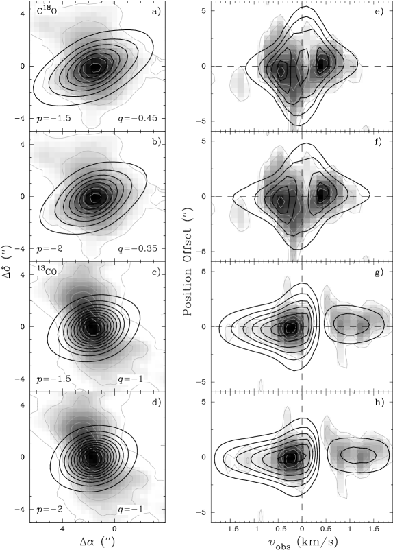
Figure 11: Modeling of envelope in C¹⁸O (a,b,e,f) and ¹³CO (c,d,g,h). Gray contours with image are the observations, black contours are derived from our simple model. (a)-(d) shows the total emission, while (e)-(h) shows the PV diagrams cut along the major axis of the flattened envelope.

There are nine parameters in this model: $H$, $R_{\textrm{\scriptsize in}}$, $R_{\textrm{\scriptsize out}}$, $n_{\textrm{\scriptsize 0}}$, $p$, $T_{\textrm{\scriptsize 0}}$, $q$, $M_{*}$, and $v_{\phi\textrm{\scriptsize 0}}$. To narrow our search, only two promising values of $p$ are considered: (1) $p=-1.5$, as found in many theoretical infalling models (see, e.g., Nakamura, 2000) and HCO⁺ observations around low-mass envelopes (Hogerheijde, 2001), and (2) $p=-2.0$, as found in 850 and 450 $\mu$m continuum observations of low-mass envelopes (Shirley et al., 2000). We find that these values of $p$ can both result in a reasonable fit to our observations too (see Fig. 11). In addition, the values of other parameters do not depend much on these values of $p$. In our fits, we have $H\sim 550$ AU ($\sim$ $1.2^{\prime\prime}$), $R_{\textrm{\scriptsize in}}\sim 115$ AU ($\sim$ $0.25^{\prime\prime}$), $R_{\textrm{\scriptsize out}}\sim 2300$ AU ($\sim$ $5^{\prime\prime}$), $M_{*}\sim 0.15$$M_{\odot}$, $v_{\phi\textrm{\scriptsize 0}}\sim 0.3$ km s^-1, and $n_{\textrm{\scriptsize 0}}\sim 4\times 10^{6}$ cm^-3. $T_{\textrm{\scriptsize 0}}$ and $q$, however, are required to be different between C¹⁸O and ¹³CO in order to fit the observations. We have $T_{\textrm{\scriptsize 0}}\sim 35$ K and $q\sim-0.4$ for C¹⁸O, and $T_{\textrm{\scriptsize 0}}\sim 23$ K and $q\sim-1$ for ¹³CO. With these values of parameters, our model can roughly reproduce: (1) the observed structures of the flattened C¹⁸O envelope and the ¹³CO waist seen around the source; (2) the observed PV structures with the emission seen across the source with the redshifted and blueshifted peaks on either side of the source; and (3) the observed redshifted dip in ¹³CO. Note that in the observations, the emission extending to the north and south is likely from the envelope material affected by the outflow shells (see §5.1) and thus is not included in our model.

The mass of the flattened envelope, which is given by

$$M_{e} = 2m_{\textrm{\scriptsize H}}n_{\textrm{\scriptsize 0}}H\int_{R_{\textrm{\scriptsize in}}}^{R_{\textrm{\scriptsize out}}}(\frac{R}{R_{\textrm{\scriptsize 0}}})^{p}2\pi RdR$$ (10)

is $\sim 0.028$ and 0.025 $M_{\odot}$ for $p=-1.5$ and $-2$, respectively. This mass, however, is a factor of 3 lower than that of the dust core. Note that the mass derived for the dust core could have an uncertainty with a factor of 5 due to the large uncertainty in the mass opacity (Beckwith et al., 1990). The infall rate, which is given by

$$\dot{M}(R) = 2\pi RHn|v_{R}|2m_{\textrm{\scriptsize H}}$$ (11)

is $\sim 6\times 10^{-6}M_{\odot}\;\textrm{yr}^{-1}$ at $R_{\textrm{\scriptsize 0}}=460$ AU.

5 Discussion

HH 212 is a highly collimated jet powered by a young Class 0 source, IRAS 05413-0104. We have mapped the jet and its source in 1.33 mm continuum, ¹²CO, ¹³CO, C¹⁸O, and SO. In the following, we discuss our results in details.

5.1 Circumstellar Envelope

A flattened envelope is seen in C¹⁸O around the source in the equator perpendicular to the jet axis, with its inner part seen in ¹³CO. The structure and kinematics of the envelope can be roughly reproduced by a simple edge-on disk model with both infall and rotation. In this model, the density of the disk is assumed to have a power-law index of $p=-1.5$ or $-2$, as found in other low-mass envelopes (Shirley et al., 2000; Hogerheijde, 2001). The temperature of C¹⁸O has a power-law index of $q\sim-0.4$, as found in other low-mass envelopes (Shirley et al., 2000; Hogerheijde, 2001). However, in order to reproduce the compact waist and the redshifted dip in ¹³CO, the temperature of ¹³CO is required to decrease with $q\sim-1$, which is faster than that of C¹⁸O. Notice that in our model, the redshifted dip is assumed to be produced by the absorption of a cold material at the outer part of the envelope. However, the dip may be partly due to missing flux in our interferometric observations (Gueth et al., 1997). Further observations and modeling (e.g., with flared disk model, turbulence, and missing flux consideration) are needed to improve this.

The envelope seems dynamically infalling toward the source with slow rotation because the kinematics is found to be roughly consistent with a free fall toward the source plus a rotation of a constant specific angular momentum. If this is the case, the source has a mass of $M_{*}\sim 0.15$ $M_{\odot}$ and the infall rate is $\sim 6\times 10^{-6}M_{\odot}\;\textrm{yr}^{-1}$ at $R_{\textrm{\scriptsize 0}}=460$ AU, similar to those found in other flattened infalling envelopes with slow rotation around low-mass protostars (Ohashi et al., 1997; Momose et al., 1998). Assuming that the accretion rate is constant in the past and given by the infall rate, the accretion time will be $M_{*}/\dot{M}\sim 3\times 10^{4}$ yr, as expected for a Class 0 source. Notice that in theoretical models (e.g., Shu et al., 2000), this accretion rate corresponds to an isothermal sound speed of 0.3 km s^-1, or equivalently a temperature of 25 K, which is consistent with our simple model. This dynamically infalling envelope with rotation is expected to form a rotationally supported disk at $R\sim 74$ AU ($\sim$ $0.16^{\prime\prime}$), at which the rotation velocity is comparable to the infall velocity (Hayashi et al., 1993; Lin et al., 1994). The ¹³CO emission seen at high velocity may arise from this rotationally supported disk, with the redshifted emission and the blueshifted emission on either side of the source (Fig. 4d).

A flattened NH₃ envelope has been seen rotating around the source in the same direction (Wiseman et al., 2001). It has a characteristic radius of $\sim$ 3500 AU ($\sim$ $8^{\prime\prime}$) and can be considered as the extension of the flattened C¹⁸O envelope into the surrounding. At that radius, the infall velocity and rotation velocity are expected to be $\sim$ 0.27 and 0.04 km s^-1, respectively in our simple model. This rotation velocity is consistent with that observed in the NH₃ envelope, suggesting that the rotation of the C¹⁸O envelope is connected to that of the NH₃ envelope, and that the angular momentum is carried inward into the C¹⁸O envelope from the NH₃ envelope. However, no infall velocity has been seen in the NH₃ envelope. In theoretical models (e.g., Shu, 1977), the infall radius is given by the isothermal sound speed times the accretion time. Assuming a temperature of 25 K, the isothermal sound speed is $\sim$ 0.3 km s^-1, resulting in an infall radius of $\sim$ 2000 AU, similar to the outer radius of the C¹⁸O envelope. Thus, it is possible that no infall motion is seen in the NH₃ envelope.

The flattened envelope is not formed by rotation because it is not rotationally supported, with the rotation velocity smaller than the infall velocity. Could it result from an interaction with the CO outflow? The flattened NH₃ envelope is seen carved by the CO outflow, forming a bowl structure around it (Wiseman et al., 2001; Lee et al., 2000). In our observations, the shells seen in C¹⁸O and ¹³CO around the bases of the nebulae may trace the (swept-up) envelope material pushed by the outflow shells toward the equator, suggesting that the envelope around the source is also carved by the outflow. Having said that, the flattened envelope may not form by the outflow interaction, because the shells are seen separated from the envelope.

Formation mechanisms of such a flattened infalling envelope around a forming star have been proposed with and without magnetic field. Galli & Shu (1993) examined the gravitational contraction of magnetized spherical cloud cores. They showed that flattened infalling envelopes are formed as the magnetic field impedes the contraction perpendicular to the field lines, which are aligned with the rotation axis. Hartmann et al. (1996) showed that even in the absence of a magnetic field, initially sheetlike cloud cores can also collapse to form flattened envelopes. Recently, Nakamura (2000) also showed that flattened infalling envelopes are a natural outcome of the gravitational contraction of prolate cloud cores with slow rotation. In this scenario, the flattened envelopes are predicted to have $n\propto r^{-1.5}$, $v_{r}\propto r^{-0.5}$, and $v_{\phi}\propto r^{-1}$, the same as our model.

5.2 Molecular Outflow

A ¹²CO outflow is seen surrounding the H₂ jet, with a narrow waist around the source. The outflow seen here in ¹²CO $J=2-1$ is similar to that seen in ¹²CO $J=1-0$, but with higher $J$ transition line of ¹²CO tracing higher velocity around the knots and bow tips. The morphological relationship between the H₂ jet and the ¹²CO outflow, and the kinematics of the ¹²CO outflow along the jet axis are both consistent with those seen in a jet-driven bow shock model (see, e.g., Lee et al., 2001, and reference therein). In that model, a highly collimated jet is launched from around the source, propagating into the ambient medium. A temporal variation in the jet velocity produces a chain of H₂ knots propagating down along the jet axis. Since these H₂ knots are localized (ballistic) shocks with high thermal pressure, they expands sideways, growing into H₂ bow shocks with the shock velocity (and thus temperature) decreasing rapidly away from the bow tips. As these bow shocks propagate down along the jet axis, they sweep up the ambient material into a thin outflow shell around the jet axis. In our observations, the ¹²CO shells around the source can be identified as the ambient material swept up by the H₂ bow shocks. In addition, ¹²CO emission also arises from around the H₂ knots and bow shocks, with the velocity decreasing rapidly away from the knots and bow tips. Higher $J$ transition line of ¹²CO traces higher velocity around the knots and bow tips likely because it arises from regions of higher temperature and thus higher velocity closer to the knots and bow tips. As a result, the ¹²CO emission appears jetlike at high velocities in high $J$ transition. Located inside the outflow cavity, the jetlike ¹²CO emission is unlikely from the entrained ambient gas. The jet is probably intrinsically molecular, such as that seen in HH 211 (Gueth & Guilloteau, 1999). Since the shell is the swept-up ambient material, the density of the ambient material is expected to be lower than that of the shell. Thus, the jet is an overdensed jet with the density higher than that of the ambient material.

In the south, ¹²CO emission is seen coincident with the H₂ bow shock SB4, indicating that the shocked material there must have cooled very fast from $\sim$ 2000 K (H₂) to a few 10 K (¹²CO) because of a significant mixing with the ambient material. The transverse velocity there is also lower than that around other bow shocks (see Fig. 7), probably because the bow shock SB4 is sharing momentum with the quiescent ambient material (cf. Fig. 7 in Lee et al., 2001). Therefore, the bow shock SB4 may trace the leading bow shock where the head of the jet impacts on the ambient material.

5.3 SO emission

SO emission is seen around the source and the H₂ knotty shocks in the south, especially the knot SK4. The emission around the source may arise from two components. Like that around the knot SK4, the emission seen at high velocity is likely to be from knotty shocks, which are expected to be there following the H₂ knotty shocks toward the source. The shocks are not seen in H₂ probably due to dust extinction. However, the SO emission seen around the systemic velocity may arise from the flattened envelope due to its low velocity. Observations at high angular resolution are needed to confirm this.

SO emission has also been seen toward the CepA-East outflows, tracing ambient material at 60-100 K and shocked gas at 70-180 K (Codella et al., 2005). Assuming an optically thin emission, a temperature of 120 K, and a SO abundance of 10^-9 relative to molecular hydrogen (Codella et al., 2005), the mass is found to be $\sim$ 0.4 and 0.1 $M_{\odot}$, respectively, around the source and the knot SK4. However, these masses are too large to be from knotty shocks. The abundance of SO must have been highly enhanced. Note that ¹²CO emission is weak around the knot SK4 (see Fig. 6b), probably suggesting that ¹²CO there is destroyed by the shock interaction. The detection of the SO emission is likely because of the abundance enhancement of SO due to the shock-triggered release of various molecules (e.g., H₂S/OCS/S) from dust mantles and the subsequent chemical reactions in the warm gas. Since the abundance is enhanced only for a very short period of time, the SO emission traces regions of recent shock activity (Codella et al., 2005).

Around the knot SK4, the redshifted emission is seen to the east while the blueshifted emission is seen to the west, similar to that seen in the flattened C¹⁸O envelope. A similar velocity structure has been seen around the knot SK1 (see Fig. 8 for its location) in H₂ and considered as a tentative evidence that the knot SK1 is rotating (Davis et al., 2000). It was observed with 3 slits from east to west with a separation of $\sim$ $0.45^{\prime\prime}$. The peak velocities with respect to the systemic velocity were found to be +4.6, +2.9, and +2.3 km s^-1, measured from east to west. Thus, assuming that the central velocity at the knot SK1 is $\sim 3$ km s^-1, the redshifted emission is seen to the east while the blueshifted is seen to the west. A similar velocity structure is seen here around the knot SK4 in SO but with higher velocity. Does this suggest that the knot SK4 is also rotating and that the jet carries away angular momentum from the infalling envelope? The velocity here, however, is much larger than $v_{\phi\textrm{\scriptsize 0}}$ (i.e., 0.3 km s^-1) and thus may be too large to be from rotation. In addition, the shocked material there is expected to have sideways expansion. Further observations at higher angular resolution are needed to study it.

6 Conclusion

We have mapped the 1.33 mm continuum, ¹²CO ($J=2-1$), ¹³CO ($J=2-1$), C¹⁸O ($J=2-1$), and SO ($J_{K}=6_{5}-5_{4}$) emission around a protostellar jet HH 212 and its central source, IRAS 05413-0104. A dust core is seen in the continuum around the source, with a temperature of $\sim$ 46 K and a mass of $\sim$ 0.08 $M_{\odot}$. A flattened envelope is seen in C¹⁸O around the source in the equator perpendicular to the jet axis, with its inner part seen in ¹³CO. The structure and kinematics of the envelope can be roughly reproduced by a simple edge-on disk model with both infall and rotation. The flattened envelope seems dynamically infalling toward the source with slow rotation because the kinematics is found to be roughly consistent with a free fall toward the source plus a rotation of a constant specific angular momentum. A ¹²CO outflow is seen surrounding the H₂ jet, with a narrow waist around the source. Jetlike structures are also seen in ¹²CO near the source aligned with the H₂ jet at high velocities. The morphological relationship between the H₂ jet and the ¹²CO outflow, and the kinematics of the ¹²CO outflow along the jet axis are both consistent with those seen in a jet-driven bow shock model. SO emission is seen around the source and the H₂ knotty shocks in the south, tracing shocked emission around them.

Table 1: Summary of Observations

Line	Frequency	Beam Size	Channel Width	Noise Levela $\sigma$
	(GHz)	(arcsec $\times$ arcsec)	(km s-1)	(Jy beam-1)
1.33 mm continuum	225.000000	2.6$\times$2.3	…	3.5E-3
12CO $J=2-1$	230.537980	2.8$\times$2.3	0.264	0.25
13CO $J=2-1$	220.398676	2.8$\times$2.4	0.274	0.15
C18O $J=2-1$	219.560357	2.8$\times$2.4	0.274	0.14
SO $J_{K}=6_{5}-5_{4}$	219.949442	2.8$\times$2.4	0.554	0.12

Figure 4: ¹³CO emission plotted on top of the H₂ image, with the asterisk indicating the IRAS source. (a) Total emission integrated over 3.4 km s^-1 from -1.7 km s^-1 to 1.7 km s^-1. The contours go from 2 to 20 $\sigma$ with a step of 3 $\sigma$, where $\sigma=0.15$ Jy beam^-1 km s^-1. (b) Low-velocity emission integrated from -0.7 to 0.7 km s^-1. The contours go from 2 to 17 $\sigma$ with a step of 3 $\sigma$, where $\sigma=0.09$ Jy beam^-1 km s^-1. (c) Low-blueshifted (blue contours) and low-redshifted (red contours) emission, integrated from -0.7 to 0 km s^-1 and 0 to 0.7 km s^-1, respectively. The contours go from 2 to 18 $\sigma$ with a step of 2 $\sigma$, where $\sigma=0.06$ Jy beam^-1 km s^-1. (d) High-blueshifted (blue contours) and high-redshifted (red contours) emission, integrated from -1.7 to -0.7 km s^-1 and 0.7 to 1.7 km s^-1, respectively. The contours go from 2 to 14 $\sigma$ with a step of 2 $\sigma$, where $\sigma=0.08$ Jy beam^-1 km s^-1.

References

- Andre et al. (2000) Andre, P., Ward-Thompson, D., & Barsony, M. 2000, Protostars and Planets IV, 59
- Beckwith et al. (1990) Beckwith, S. V. W., Sargent, A. I., Chini, R. S., & Guesten, R. 1990, AJ, 99, 924
- Chapman et al. (2002) Chapman, N. L., Mundy, L. G., Lee, C.-F., & White, S. M. 2002, Bulletin of the American Astronomical Society, 34, 1133
- Chini et al. (1997) Chini, R., Reipurth, B., Sievers, A., Ward-Thompson, D., Haslam, C. G. T., Kreysa, E., & Lemke, R. 1997, A&A, 325, 542
- Claussen et al. (1998) Claussen, M.J., Marvel., K.B., Wootten, A., Wilking, B.A. 1998, ApJL, 507, L79
- Codella et al. (2005) Codella, C., Bachiller, R., Benedettini, M., Caselli, P., Viti, S., & Wakelam, V. 2005, MNRAS, 361, 244
- Davis et al. (2000) Davis, C. J., Berndsen, A., Smith, M. D., Chrysostomou, A., & Hobson, J. 2000, MNRAS, 314, 241
- Evans (1999) Evans, N. J. 1999, ARA&A, 37, 311
- Frerking et al. (1982) Frerking, M. A., Langer, W. D., & Wilson, R. W. 1982, ApJ, 262, 590
- Galli & Shu (1993) Galli, D., & Shu, F. H. 1993, ApJ, 417, 243
- Galván-Madrid et al. (2004) Galván-Madrid, R., Avila, R., & Rodríguez, L. F. 2004, Revista Mexicana de Astronomia y Astrofisica, 40, 31
- Gibb et al. (2004) Gibb, A. G., Richer, J. S., Chandler, C. J., & Davis, C. J. 2004, ApJ, 603, 198
- Gueth et al. (1997) Gueth, F., Guilloteau, S., Dutrey, A., & Bachiller, R. 1997, A&A, 323, 943
- Gueth & Guilloteau (1999) Gueth, F. & Guilloteau, S. 1999, A&A, 343, 571
- Hartmann et al. (1996) Hartmann, L., Calvet, N., & Boss, A. 1996, ApJ, 464, 387
- Hayashi et al. (1993) Hayashi, M., Ohashi, N., & Miyama, S. M. 1993, ApJ, 418, L71
- Hogerheijde (2001) Hogerheijde, M. R. 2001, ApJ, 553, 618
- Lee et al. (2000) Lee, C.-F., Mundy, L.G., Reipurth, B., Ostriker, E.C., & Stone, J.M. 2000, ApJ, 542, 925
- Lee et al. (2001) Lee, C.-F., Stone, J. M., Ostriker, E. C., & Mundy, L. G. 2001, ApJ, 557, 429
- Lin et al. (1994) Lin, D. N. C., Hayashi, M., Bell, K. R., & Ohashi, N. 1994, ApJ, 435, 821
- McCaughrean et al. (2002) McCaughrean, M., Zinnecker, H., Andersen, M., Meeus, G., & Lodieu, N. 2002, The Messenger, 109, 28
- Momose et al. (1998) Momose, M., Ohashi, N., Kawabe, R., Nakano, T., & Hayashi, M. 1998, ApJ, 504, 314
- Nakamura (2000) Nakamura, F. 2000, ApJ, 543, 291
- Ohashi et al. (1997) Ohashi, N., Hayashi, M., Ho, P. T. P., & Momose, M. 1997, ApJ, 475, 211
- Shirley et al. (2000) Shirley, Y. L., Evans, N. J., Rawlings, J. M. C., & Gregersen, E. M. 2000, ApJS, 131, 249
- Shu (1977) Shu, F. H. 1977, ApJ, 214, 488
- Shu, Adams, & Lizano (1987) Shu, F. H., Adams, F. C., & Lizano, S. 1987, ARA&A, 25, 23
- Shu et al. (2000) Shu, F.H., Najita, J., Shang, H., & Li, Z. -Y. 2000, in Protostars and Planets IV, ed. V. Mannings, A. P. Boss & S. S. Russell (Tucson: University of Arizona Press), in press
- Wiseman et al. (2001) Wiseman, J., Wootten, A., Zinnecker, H., & McCaughrean, M. 2001, ApJ, 550, L87
- Zinnecker, McCaughrean, & Rayner (1998) Zinnecker, H., McCaughrean, M. J. & Rayner, J. T. 1998, Nature, 394, 862
- Zinnecker et al. (1992) Zinnecker, H. , Bastien, P. , Arcoragi, J. -P. & Yorke, H. W. 1992, A&A, 265, 726