Searching For Integrated Sachs-Wolfe Effect Beyond Temperature Anisotropies: CMB E-mode Polarization-Galaxy Cross Correlation

Abstract

The cross-correlation between cosmic microwave background (CMB) temperature anisotropies and the large scale structure (LSS) traced by the galaxy distribution, or sources at different wavelengths, is now well known. This correlation results from the integrated Sachs-Wolfe (ISW) effect in CMB anisotropies generated at late times due to the dark energy component of the Universe. In a reionized universe, electron scattering at low redshifts leads to a large-scale polarization contribution. In addition to the primordial quadrupole, involving anisotropies at the last scattering surface, the ISW quadrupole rescatters and contributes to the large angular scale polarization signal. Thus, in principle, the low multipole polarization bump in the E-mode should be correlated with the galaxy distribution. Unlike CMB temperature—LSS correlation that peaks for tracers at low redshifts, due to the increasing visibility function, while the fractional ISW quadrupole is decreasing, with increasing redshift, the polarization—galaxy correlation peaks mostly at redshifts between 1 and 3. Under certain conditions, mostly involving a low optical depth to reionization if the Universe reionized at a redshift around 6, the cross polarization—source signal is marginally detectable if all-sky maps of the large scale structure at redshifts between 1 and 3 is available. If the Universe reionized at a redshift higher than 10, it is unlikely that this correlation will be detectable even with no instrumental noise all-sky maps. While our estimates do not guarantee a detection, unknown physics related to the dark energy uncertain issues related to the large angular scale CMB and polarization anisotropies, and uncertainties related to the reionization history of the Universe may motivate attempts to measure this correlation using upcoming CMB polarization E-mode maps and large-scale structure maps of the high-redshift universe with Large Synoptic Survey Telescope and quasar catalogs, among others.

1 Introduction

At large angular scales, in addition to primordial cosmic microwave background (CMB) anisotropies generated at the last scattering surface, the integrated Sachs-Wolfe (ISW; Sachs & Wolfe 1967) effect also provides an additional contribution at late times. The temperature fluctuations in the ISW effect results from the differential redshift effect from photons climbing in and out of time evolving potential perturbations from last scattering surface to present day. In currently popular cold dark matter cosmologies with a cosmological constant, significant contributions to temperature anisotropies arise at redshifts less than 1 and on and above the scale of the horizon at the time of decay. It is then expected that the ISW effect is correlated with the large scale structure (e.g., Crittenden & Turok 1996). Since the ISW contribution is sensitive to how one models cosmology at late-times, such as the presence of a dark energy component or not, the correlation between the ISW effect and the tracers of the large scale structure has been suggested as a probe of the dark energy properties (Corasaniti et al. 2003; Hu & Scranton 2004; Garriga et al. 2004; Pogosian 2004; Pogosian et al. 2005).

Several attempts have now been made to detect the correlation between the ISW effect, as traced by CMB maps of the Wilkinson Microwave Anisotropy Probe (WMAP; Bennett et al. 2003), and sources at optical (Scranton et al. 2003; Padmanabhan et al. 2005; Afshordi et al. 2004; Fosalba & Gaztanaga 2004; Fosalba et al. 2003), X-ray, and radio (Nolta et al. 2004; Boughn & Crittenden 2004) wavelengths. Detections are at the level of 2 to 3 $\sigma$ depending on what sources are used and what their redshift distributions are, among other parameters related to the tracer field and whether the statistic is in Fourier space or real space. These detections have allowed certain constraints on dark energy parameters (e.g., Corasaniti et al. 2005) and additional applications such as a way to slightly improve the tensor-to-scalar ratio (Cooray et al. 2005). Looking for additional signatures of the ISW effect (e.g., Cooray & Baumann 2003) is useful to further improve our understanding of dark energy

While temperature anisotropies have been used so far to look for the ISW effect, it is possible that CMB polarization anisotropies also contain signature of time-evolving potential perturbations at low redshifts compared to the redshift of last scattering. Linear polarization of the CMB is generated essentially through rescattering of the temperature quadrupole (Rees 1968). At the last scattering surface, this leads to the primordial polarization contribution (e.g., Hu & White 1997), while at lower redshifts, the temperature quadrupole gets scattered again when the Universe reionizes. This late-time reionization contribution generates a large angular scale polarization corresponding to the angular scale of the horizon at the surface of reionization (Zaldarriaga 1997).

This apparent excess of polarization at large angular scales, as expected in a reionized Universe at late-times, has now been detected with WMAP using the temperature-polarization cross power spectrum (Kogut et al. 2003). Models of this signal including other cosmological parameters indicate that the optical depth to reionization is around $\tau\sim 0.17$ such that the redshift of reionization is around 20. However, there are large degeneracies between the optical depth and other parameters as well as large uncertainties resulting from the low signal-to-noise level of this detection. Moreover, foregrounds in the CMB polarization maps are yet to be characterized properly. The expected improvements of WMAP data over the next few years as well as the planned Planck experiment will significantly improve the signal-to-noise level of CMB polarization maps in the near future.

Since the temperature anisotropy quadrupole is rescattered to generate a polarization signal, the large angular scale polarization signal, in principle, should contain the quadrupole generated by the ISW effect in addition to the dominant quadrupole associated with primordial fluctuations at the last scattering surface. Again, in principle, large angular scale polarization should be correlated with tracer fields of the large-scale structure at which the polarization signal related ISW quadrupole is generated. Since the scattering probability increases with increasing redshift while the ISW contribution is decreasing, unlike temperature anisotropies from the ISW that peak at redshifts $<1$ (Cooray 2002b; Afshordi 2004), ISW polarization contribution is expected to peak at a slightly higher redshift. Thus, tracer fields at redshifts $\sim$ 1 to 3 are more likely to be suitable for the cross-correlation.

However, a reliable detection of this cross-correlation must overcome several challenges. For example, a large fraction of the polarization signal is generated by scattering of the primordial quadrupole involving potential perturbations at the last scattering surface associated with the Sachs-Wolfe (SW) effect. To detect the ISW effect in the form of a cross-correlation with sources at the ideal redshift range, SW contribution to polarization should be smaller such that the cumulative polarization is not dominated by primordial quadrupole but rather by the late-time ISW. In the case of temperature anisotropies, in certain cosmological models, the SW and ISW contributions to large angular scales CMB anisotropies are at the same order of magnitude. In the case of polarization, the ISW contribution to the large angular scale signal is at the level of $\sim$ 0.01 $\mu$K or below, depending on the background cosmology. In comparison, if the optical depth to reionization is $\tau>0.08$, the scattering of the primordial quadrupole lead to a polarization signal higher than 0.1 $\mu$K. Thus, the detection of ISW contribution in polarization is challenging since the primordial polarization results in a large noise source within which correlations with tracer fields are measured.

The detection may be facilitated under certain conditions. For example, if the overall optical depth to reionization is small, say if reionization was at a redshift around 6 as suggested by some of the optical observations (e.g., Fan et al. 2001; White et al. 2003), then the ratio of ISW-to-SW signal in the polarization would be higher, say when compared to a universe reionized at a redshift greater than 10. Assuming standard LCDM cosmology with the dark energy described by a cosmological constant, based on the numerical calculations presented here, we find that it is possible to make a marginal detection of the ISW signal in polarization in this case. There may be other possibilities that increase the signal-to-noise ratio of the detection. If dark energy, which is marginally understood with current data, could behave in a way that it’s behavior leads to a slightly higher ISW contribution at higher redshifts than expected in models of a cosmological constant. While we have not investigated such a possibility here, various models that are developed in the literature could potentially be tested. The third possibility that may improve a detection is changes to the primordial quadrupole than what is expected in standard cosmological models. For example, large angular scale anomalies in CMB temperature anisotropy data, both from COBE and WMAP, suggests an apparent lack of primordial power at largest angular scales (e.g., Spergel et al. 2003; Efstathiou 2003; Copi et al. 2005). Such a decrease in power is expected to make slight modifications to the polarization signal and to result in a lower polarization signal at large angular scales than assumed with no modifications to the primordial spectrum (e.g., Cline et al. 2003). In fact, CMB polarization towards galaxy clusters may provide a mechanism to look for the cut-off in primordial power spectrum (e.g., Baumann & Cooray 2003; Seto & Pierpaoli 2005). If there is a cut-off in the spectrum at small scales, ISW signal remain unaffected and the ratio of ISW-to-SW contribution to polarization may be higher when compared to a model where large-scale power is not affected. Thus, we find that there are good motivations to look for the ISW signature in polarization anisotropies through cross-correlations with sources in addition to same studies with temperature anisotropy maps alone.

This paper is organized as following: in the next Section, we briefly summarize the ISW signal in CMB polarization at large angular scales and the cross-correlation between a tracer field of the large scale structure such as galaxies. We also estimate signal-to-noise levels for a detection of this correlation and show that the overall detectability is marginal, with a signal-to-noise ratio of about 2 with all-sky maps of the tracer field, if the universe reionized at a redshift around 6. This ratio could potentially improve in certain models of dark energy, especially ones where a significant derivative exists for the dark energy equation of state at redshifts between 1 to 3. Moreover, the detectability may also improve under conditions where the primordial contribution is smaller, such as in models where the large-scale power has a cut-off; Though numerical calculations with a cut-off show that the overall increase in the signal-to-noise ratio is insignificant since it only boosts the correlation level of lowest order multipoles. Finally, the signal-to-noise ratio we quote is for the detection in terms of the angular cross power spectrum between galaxies and the polarization E-mode, techniques could be improved to detect this cross signal in pixel space or using other data analysis techniques where the primordial contribution is accounted for and filtered out. We conclude with a summary of our results. For illustration purposes, we assume a cosmological model with $\Omega_{m}=0.25$, $\Omega_{\Lambda}=0.75$, $h=0.72$, and a normalization to the power spectrum of $\sigma_{8}=1.0$.

2 Calculational Method

To describe the existence of a correlation, we first summarize the ISW contribution to CMB anisotropies. The ISW effect (Sachs & Wolfe 1967) results from the late time decay of gravitational potential fluctuations. The resulting temperature fluctuations in the CMB can be written as

$$T^{ISW}(\hat{\bf n})=-2\int_{0}^{{r}_{s}}d{r}\dot{\Phi}({r},\hat{\bf n}{r})\,,$$ (1)

where the overdot represent the derivative with respect to conformal distance (or equivalently look-back conformal time) and $\Phi({r},\hat{\bf n}{r}))$ is the potential perturbations in the large-scale structure. Here, ${r}_{s}$ is the radial distance to the last scattering surface.

Writing multipole moments of the temperature fluctuation field $T(\hat{\bf n})$,

$$a_{lm}=\int d\hat{\bf n}T(\hat{\bf n}){Y_{lm}}{}^{*}(\hat{\bf n})\,,$$ (2)

we can formulate the angular power spectrum as

$$\langle a_{l_{1}m_{1}}^{*}a_{l_{2}m_{2}}\rangle={\delta^{D}}_{l_{1}l_{2}}{\delta^{D}}_{m_{1}m_{2}}C_{l_{1}}\,.$$ (3)

For the ISW effect, multipole moments are

$$a^{\rm ISW}_{lm} = i^{l}\int\frac{d^{3}{\bf k}}{2\pi^{2}}\int d{r}\delta({\bf k})I_{l}(k){Y_{lm}}(\hat{{\bf k}})\,,$$

with $I_{l}(k)=\int d{r}W^{ISW}(k,{r})j_{l}(k{r})$ with the window function for the ISW effect

$$W^{ISW}(k,{r})=-3\Omega_{m}\frac{H_{0}^{2}}{k^{2}}\frac{d}{d{r}}\left(\frac{G}{a}\right)\,.$$ (5)

Here, we have made use of the Poisson equation to related potential fluctuations to the density field and have assumed linear perturbations with the growth factor given by $G({r})$ (see, Cooray 2002b for details). We ignore non-linear corrections to the ISW effect since they only lead to anisotropies at small scales and do not modify the quadrupole (Cooray 2002a). The function $d/dr(G/a)$ is strongly sensitive to dark energy density and related parameters, while zero in an Einstein-de Sitter universe with $\Omega_{m}=1$. As is well-known the overall ISW contribution provides a sensitive probe of dark energy. In fact, as discussed in Cooray et al. (2004), if the ISW contribution can be established as a function redshift, it provides a more powerful probe of dark energy than estimates involving luminosity distances and other cosmological probes (assuming they are also measured to the same accuracy as a function of redshift).

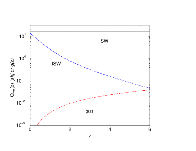
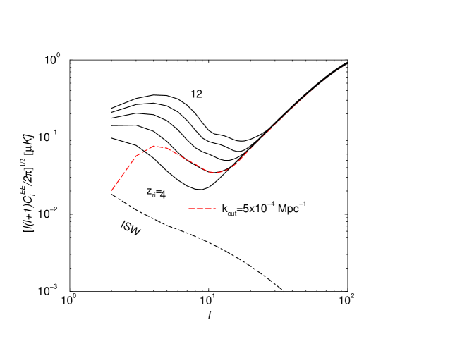
Figure 1: Left panel: The rms quadrupole as a function of redshift. The top horizontal line is the primordial quadrupole related to SW effect while the long-dashed line shows the ISW contribution that peak as the redshift is decreased. For comparison on the redshift dependence, with dot-dashed line we also show $g(z)$, the visibility function that determine the scattering probability. This function increases as the redshift is increased, but sharply drops to zero beyond the redshift at which the Universe reionized. Most of the scattering happens at the reionization redshift and the resulting polarization signal is dominated by scattering of the primordial quadrupole. Right panel: The polarization anisotropy power spectrum, in the E-mode, as a function of the multipole and as a function of the reionization redshift, from 4 to 12 at steps of 2. Note that the ISW contribution is significantly smaller than the contribution from SW quadrupole scattering. In fact, the ratio of ISW-to-SW contributions to polarization decreases as the reionization redshift is increased. A favorable detection of the ISW effect in polarization, through a cross-correlation, generally require a low optical depth or a reionization redshift $\sim$ 6. For reference, we also show the case where the primordial power spectrum has a cut-off at wavenumbers below $5\times 10^{-4}$ Mpc^-1, as required to explain the low power of the temperature anisotropy quadrupole and the octupole (Kesden et al. 2003).

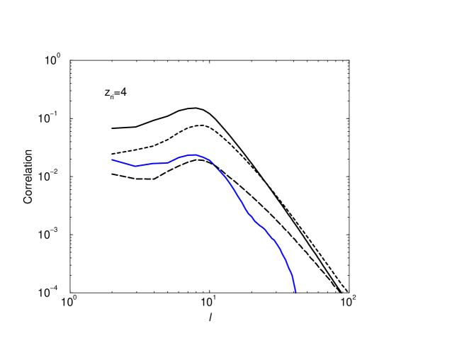
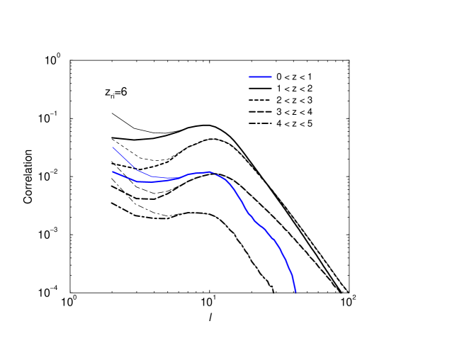
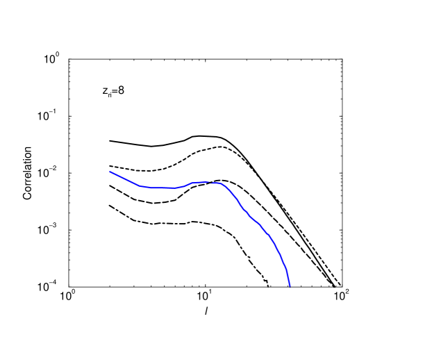
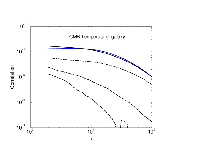
Figure 2: The correlation coefficient $r$ between E-mode polarization maps and a tracer field, as a function of the redshift bin of the source field. From top-left to bottom-left we show correlation coefficients assuming a reionization redshift of 4, 6, and 8, respectively. The bottom-right panel shows the correlation coefficient between CMB temperature anisotropy maps and tracer fields again divided to redshift bins as indicated on the top right panel. The correlations peak at a multipole $\sim 10$ and decreases sharply thereafter due to the increase in $C_{l}^{\rm EE}$ when $l>10$ (see. Figure 1 right panel). In the case of polarization, correlation coefficients are higher for tracer fields at redshifts between 1 and 3, relative to coefficients for sources between redshifts of 0 and 1. This can be compared to temperature-source correlation which peaks for sources between redshifts of 0 and 2. In the top right panel, thin lines show the correlation coefficient with a cut-off in the power spectrum (see, Figure 1 right panel).

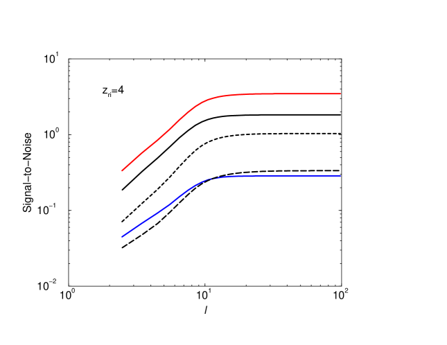
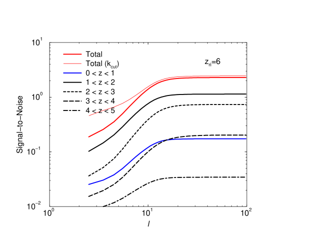
Figure 3: The cumulative signal-to-noise ratio for a detection of the E-mode polarization-source correlations as a function of the multipole. The signal-to-noise ratios peak at a multipole around $\sim$ 10. The two panels assume a reionization redshift of 4 and 6, while for a reionization redshift 8 and higher the total signal-to-noise ratio is below unity. The tracer field is divided to redshift bins as labeled on the right panel assuming tracers, such as galaxies, are uniformly distributed in that bin. We assume a source bias of unity with respect to the linear density field regardless of the redshift; high redshift sources are likely to have a bias factor greater than unity (see, for example, Figure 15 of Cooray 2005) and could aid the detection, but we do not pursue such possibilities here; An increase in the bias factor is likely to be compensated by the decreasing density of high-redshift sources. The signal-to-noise ratios plotted here assuming all-sky maps, but for partial sky coverage, these numbers decrease as $\sqrt{f_{\rm sky}}$, but coverages less than $\sim$ 50 by 50 degrees are not useful as they do not adequately probe multipoles $\sim$ 10. In the right panel, the thin line shows the signal-to-noise ratio with a cut-off in the primordial power spectrum. A cut-off at a wave number of $5\times 10^{-4}$ Mpc^-1 only results in a small increase in the overall signal-to-noise ratio and a cut-off alone would not significantly boost the ISW-source correlation using polarization maps to a level where the detection is guaranteed.

For comparison, the angular power spectrum of temperature anisotropies is then given by

$$C_{l}^{ISW}={2\over\pi}\int k^{2}dkP(k)\left[I_{l}^{\rm ISW}(k)\right]^{2}\,,$$ (6)

while the cross-correlation between sources and temperature is simply

$$C_{l}^{{ISW}-gal}={2\over\pi}\int k^{2}dkP(k)I_{l}^{\rm ISW}(k)I_{l}^{\rm gal}(k)\,,$$ (7)

where

$$I_{l}^{\rm gal}(k)=\int d{r}b(k,{r})n^{\rm gal}({r})j_{l}(k{r})$$ (8)

where $n^{\rm gal}({r})$ is the normalized radial distribution of sources (such that $\int drn^{\rm gal}({r})=1$) and $b(k,{r})$ is the scale dependent bias factor of these sources relative to the linear density field. In this calculation, we will assume sources are uniformly distributed in redshift and can be divided to redshift bins from 0 to 5 at steps of unity. We will assume the bias factor is scale independent and has a value of unity. Since our calculation is mostly for illustrative purposes to obtain the order of magnitude estimate of the detectability level of the ISW polarization-galaxy cross-correlation these assumptions are adequate.

The polarization signal is generated by rescattering of the temperature quadrupole. We consider the E-mode here since that is induced by scalar fluctuations. Following Zaldarriaga (1997), the large scale angular power spectrum of the E-mode polarization is

$$C_{l}^{EE}={2\over\pi}\int k^{2}dkP(k)[I_{l}^{\rm E}(k)]^{2}\,,$$ (9)

where

$$I_{l}^{\rm E}(k)=\sqrt{\frac{(l+2)!}{(l-2)!}}\frac{3}{4}\int d{r}g({r})Q(k,{r})\frac{j_{l}(k{r})}{(k{r})^{2}}$$ (10)

where $g({r})=\int d{r}\dot{\tau}e^{-\tau}$ is the visibility function that determines the scattering probability and the quadrupole that rescatters via electrons in a reionized Universe has two contributions

$$Q(k,{r}) = Q^{\rm SW}(k,{r})+Q^{\rm ISW}(k,{r})$$ (11)

$$Q^{\rm SW}(k,{r}) = -\frac{1}{2}\Omega_{m}\frac{H_{0}^{2}}{k^{2}}\left(\frac{G}{a}\right)_{{r}_{s}}j_{2}[k({r}_{s}-{r})]$$

$$Q^{\rm ISW}(k,{r}) = -3\Omega_{m}\frac{H_{0}^{2}}{k^{2}}\int_{{r}}^{{r}_{s}}d{r}^{\prime}\frac{d}{d{r}^{\prime}}\left(\frac{G}{a}\right)j_{2}[k({r}^{\prime}-{r})]\,.$$ (12)

In the same manner we described the CMB temperature and source cross-correlation, we can also write the cross-correlation between a tracer field of the large-scale structure and polarization anisotropies as

$$C_{l}^{E-gal}={2\over\pi}\int k^{2}dkP(k)I_{l}^{\rm E-ISW}(k)I_{l}^{\rm gal}(k)\,,$$ (13)

where the source related to polarization is now the ISW effect only (such that in equation 10, the quadrupole $Q(k,{r})$ is replaced by $Q^{\rm ISW}(k,{r})$ from equation 12).

In Figure 1 (left panel), we show the rms quadrupole of SW and ISW effects as a function of redshift. These rms quadrupoles (Hu 1999; Baumann et al. 2003) are calculated through

$$Q_{\rm rms}^{2}({r})=\int\frac{k^{2}dk}{2\pi^{2}}Q^{2}(k,{r})\,.$$ (14)

For comparison, in Figure 1, we also show the function $g({r})$. The rms quadrupoles, as a function of redshift, show the general behavior of the primordial contribution (SW) and the relative effect from the ISW effect to CMB polarization. While the ISW contribution decrease with increasing redshift, the scattering probability increases. On the other hand, rms SW quarupole is essentially the same regardless of redshift; on the otherhand, due to changes in the size of the last scattering surface an electron sees at high redshift, $Q^{\rm SW}(k,{r})$ does change as a function of redshift when considered as a function of the wavenumber (for example, see Baumann & Cooray 2003; Seto & Pierpaoli 2005). Thus, if the scattering were to begin at a higher redshift, the overall contribution to polarization would be higher and be dominated by the SW quadrupole. As long as the reionization redshift is greater than 4, the ISW contribution is no more than 0.01 $\mu$K, while the SW contribution is at the level of 0.1 $\mu$K or higher depending on the exact redshift of reionization (see, Figure 1 right panel).

For comparison between the temperature and polarization cross-correlation signals, it is useful to consider the cross-correlation coefficient $r$ between CMB signals and the tracer field. In the case of temperature-galaxy correlation, this coefficient is

$$r_{\rm temp}=\frac{C_{l}^{{ISW}-gal}}{\sqrt{C_{l}^{\rm temp}C_{l}^{\rm gal}}}$$ (15)

where $C_{l}^{\rm temp}$ is total power spectrum of temperature fluctuations and $C_{l}^{\rm gal}$ is the power spectrum of sources. Similarly, for polarization, this correlation is

$$r_{\rm pol}=\frac{C_{l}^{E-gal}}{\sqrt{C_{l}^{EE}C_{l}^{\rm gal}}}\,,$$ (16)

where now $C_{l}^{EE}$ is all contributions to polarization both from rescattering at a reionized Universe and from last scattering surface.

In Figure 2, we summarize the correlation coefficients for polarization-source cross-correlation detection for three assumed values of the reionization redshift:4, 6, 8. While it is clear that reionization happened at a redshift greater than 6, we use $z_{\rm ri}=4$ for illustrative purposes here. In the same figure, we also show the correlation coefficient related to temperature-source detection (bottom right panel). The correlation coefficient in this case is at the level of $0.2$ for sources at redshifts less than unity. On the other hand, the correlation coefficient is smaller ($<0.1$) for polarization-source correlation when $z_{\rm ri}\geq 6$. These correlations peak for sources with redshifts between 1 and 2. Sources with redshifts between 2 and 3 have a larger correlation relative to sources between redshifts 0 and 1. Unlike the case with temperature-source correlation coefficients, as a function of the multipole where one sees a broad range in multipole values for essentially the same coefficient, the correlation coefficient for polarization-source case decreases rapidly when $l>10$ due to the sharp rise in the polarization power spectrum (see, Figure 1) associated with primordial polarization generated by the velocity gradients at the last scattering surface. The correlation coefficient is, in fact, higher around a multipole of 10 due to the “dip” in the EE polarization power spectrum.

The above comparison indicates that the detection of the polarization-source cross power spectrum may be challenging, and to quantify this further, we also estimate the signal-to-noise ratio for its detection

$$\left(\frac{\rm S}{\rm N}\right)^{2}=\sum_{l}f_{\rm sky}(2l+1)\frac{\left(C_{l}^{E-gal}\right)^{2}}{C_{l}^{E-gal}+\left(C_{l}^{\rm EE}+C_{l}^{\rm noise}\right)\left(C_{l}^{\rm gal}+N_{l}^{\rm gal}\right)}\,.$$ (17)

To estimate the maximal signal-to-noise ratio, we ignore noise in CMB polarization map, $C_{l}^{\rm noise}$, and shot-noise of galaxies, $N_{l}^{\rm gal}$, and concentrate only on the cosmic variance. This is a safe assumption that at angular scales or multipoles where this correlation peaks, $l\sim 10$, CMB maps will eventually become cosmic-variance limited (such as the case now for temperature with WMAP) and, again, shot-noise from sources are not a significant concern. In Figure 3, we show the cumulative signal-to-noise ratios as a function of the increasing multipole. As expected the signal-to-noise ratios peak at a multipole around 10 and when all redshift bins are summed, the total is at the level of $\sim$ 3 ($z_{\rm ri}=4$) and 2 ($z_{\rm ri}=6$) and drops below unity when $z_{\rm ri}>10$. These signal-to-noise levels assume all-sky maps of the tracer field and for partial sky coverage, the ratios decrease as $\sqrt{f_{\rm sky}}$. Even for all-sky maps, the detection of the cross polarization-source signal is marginal.

This signal-to-noise ratio, however, is not significantly less than unity. This suggests that, while marginal, other reasons may determine if the correlation can be detected or not. For example, while we have not explored the large range of models suggested for dark energy, there may be a favorable dark energy model already in the literature or reasonably conceived to “boost” the ISW signal at redshifts between 1 and 3. Similarly, $C_{l}^{\rm EE}$ may be smaller at small multipoles if some suggestions related to the apparent lack of power in CMB temperature maps were to hold, such as those involving a cut-off. In Figure 1, we show an example case where we consider the primordial power to be zero at wavenumbers $k_{\rm cut}<5\times 10^{-4}$ Mpc^-1. Such a cut-off explains the apparent low power of the quadrupole and the octupole of the temperature anisotropy maps (e.g., Kesden et al. 2003). While a better characterization of the cut-off, if it exists, may be interesting to understand physics during the early Universe (e.g., Hannestad & Mersini-Houghton 2005), techniques to further study it are limited (Kesden et al. 2003). The ISW-polarization cross-correlation may provide additional information, though we find that the overall increase in the signal-to-noise ratio with a cut-off is not significant. Finally, while we have considered the angular cross power spectrum, there may be more suitable techniques to look for the ISW polarization-source correlations. Such techniques could involve looking for correlations directly in the pixel space, techniques to account for primordial signal in the polarization map based on additional correlations, among others.

Any attempts to detect this correlation also require wide-field maps of the large-scale structure at redshifts between 1 and 3. While such information already exists at low redshifts, with surveys such as the Sloan Digital Sky Survey, high redshift maps will soon become available with planned sky surveys with instruments such as the Large Synoptic Survey Telescope (LSST; Tyson et al. 2002). Studies on how large-scale structure involving billion or more galaxies from LSST can be applied for astrophysical and cosmological studies are already underway (e.g., Zhan et al. 2005). Improved polarization maps, from WMAP data and the upcoming Planck mission, can easily be combined with imaging data from LSST, especially on large-scale structure around redshifts 1 to 3, to look for the suggested cross-correlation. In addition to galaxies, sources that span the required redshift ranges include quasars and AGNs at other wavelengths. While the detection requires favorable conditions even a non detection may be useful to constrain properties of dark energy at such high redshifts. This is also useful again in the context that most other cosmological probes of dark energy, such as galaxy cluster number counts, consider redshifts below unity or out to at most 1.7 (such as Type Ia supernovae).

Beyond dark energy, this test has the most power in constraining the overall redshift of reionization. For example, a detectable signal would generally require that the Universe reionized at a late time, such as through quasars at a redshift $\sim 6$. On the other hand current determinations of the optical depth argue for a much higher redshift for reionization with optical depth $\sim$ 0.17. The latter has large uncertainties both in the measurements as well as in the interpretation through degeneracies between other parameters. With high signal-to-noise E-mode polarization maps cross-correlation studies can be considered and if a detection were to be found, this should generally argue for a low reionization redshift.

3 Conclusions

The cross-correlation between cosmic microwave background (CMB) temperature anisotropies and the large scale structure (LSS) traced by the galaxy distribution, or sources at different wavelengths, is now well known. This correlation results from the integrated Sachs-Wolfe (ISW) effect in CMB anisotropies and provides a measure of dark energy and its physical properties. In a reionized universe, electron scattering at low redshifts leads to a large-scale polarization contribution. In addition to the primordial quadrupole, involving anisotropies at the last scattering surface, the ISW quadrupole rescatters and contributes to large-scale polarization signal. Thus, in principle, the large-scale polarization bump in the E-mode should also be correlated with the galaxy distribution. Unlike CMB-LSS correlation that peaks for tracers at low redshifts, due to the decreasing visibility function at low redshifts and the decreasing ISW contribution at high redshifts, the correlation peaks mostly at redshifts between 1 and 3. Under certain conditions, mostly involving a low optical depth to reionization, the polarization signal should be detectable, though signal-to-noise ratios involving an all-sky map of the galaxy distribution is not expected to be high and is likely to be at the level of two to three if the Universe reionized at a redshift around 6. If the Universe reionized at a redshift higher than 8, it is unlikely that this correlation will be detectable. Unknown physics related to the dark energy as well as still uncertain issues related to the large angular scale CMB and polarization anisotropies, however, may compel attempts to measure this correlation using upcoming CMB polarization E-mode maps.

4 Acknowledgments

We thank Levon Pogosian, Pier-Stefano Corasaniti, and Niyesh Afshordi for useful comments on an early draft of this paper. AM is supported by MURST through COFIN contract no. 2004027755.

References

References

- [1] N. Afshordi, Phys. Rev. D 70, 083536 (2004).
- [2] N. Afshordi, Y. Loh and M.A. Strauss, Phys. Rev. D69, 083542 (2004).
- [3] D. Baumann, A. Cooray and M. Kamionkowski, New Astron. 8, 565 (2003) [arXiv:astro-ph/0208511].
- [4] D. Baumann and A. Cooray, New Astron. Rev. 47, 839 (2003) [arXiv:astro-ph/0304416].
- [5] C. Bennett, et al., Astrophys. J. Supp. 148, 97 (2003).
- [6] S. Boughn and R. Crittenden, Nature 427, 45 (2004).
- [7] J. M. Cline, P. Crotty and J. Lesgourgues, 2003, JCAP, 0309, 10 (2003).
- [8] C. J. Copi, D. Huterer, D. J. Schwarz & G. D. Starkman, 2005, MNRAS submitted (astro-ph/0508047)
- [9] A. Cooray, Phys. Rev. D65, 103510 (2002a), astro-ph/0112408.
- [10] A. Cooray, Phys. Rev. D., 65, 083518 (2002b), astro-ph/0109162.
- [11] A. Cooray, arXiv:astro-ph/0506087.
- [12] A. Cooray, D. Huterer and D. Baumann, Phys. Rev. D69, 027301 (2004), astro-ph/0304268.
- [13] A. Cooray and D. Baumann, Phys. Rev. D 67, 063505 (2003).
- [14] A. Cooray, P. S. Corasaniti, T. Giannantonio and A. Melchiorri, Phys. Rev. D 72, 023514 (2005) [arXiv:astro-ph/0504290].
- [15] P.S. Corasaniti, B.A. Bassett, C. Ungarelli and E.J. Copeland, Phys. Rev. Lett.90, 091303 (2003).
- [16] P. S. Corasaniti, T. Giannantonio and A. Melchiorri, Phys. Rev. D 71, 123521 (2005). astro-ph/0504115.
- [17] R. Crittenden and N. Turok, Phys. Rev. Lett.76, 575 (1996).
- [18] G. Efstathiou, Mon. Not. Roy. Astron. Soc. 343, L95 (2003) [arXiv:astro-ph/0303127].
- [19] X. Fan, V. K. Narayanan, M. A. Strauss, R. L. White, R. H. Becker, L. Pentericci and H. W. Rix, arXiv:astro-ph/0111184;
- [20] P. Fosalba and E. Gaztanaga, Mon. Not. R. Astron. Soc. 350, L37 (2004).
- [21] P. Fosalba, E. Gaztanaga and F.J. Castander, ApJ89, L597 (2003).
- [22] J. Garriga, L. Pogosian and T. Vachaspati, Phys. Rev. D69, 063511 (2004).
- [23] S. Hannestad and L. Mersini-Houghton, Phys. Rev. D 71, 123504 (2005) [arXiv:hep-ph/0405218].
- [24] W. Hu and R. Scranton, Phys. Rev. D70, 123002 (2004).
- [25] W. Hu and M. White, New Astron, 2, 323 (1997).
- [26] W. Hu, Astrophys. J. 529, 12 (2000) [arXiv:astro-ph/9907103].
- [27] M. H. Kesden, M. Kamionkowski and A. Cooray, Phys. Rev. Lett. 91, 221302 (2003) [arXiv:astro-ph/0306597].
- [28] A. Kogut, et al. Astrophys. J. Supp. 148, 161 (2003).
- [29] L. Pogosian, astro-ph/0409059.
- [30] L. Pogosian, P.-S. Corasaniti, C. Stephan-Otto, R. Crittenden and R. Nichol, Phys. Rev. D in press (astro-ph/0506396)
- [31] M.R. Nolta et al., ApJ608, 10 (2004).
- [32] N. Padmanabhan, C. H. Hirata, U. Seljak, D. Schlegel, J. Brinkmann, and D. P. Schneider, 2005, Phys. Rev. D 72, 043525 (2005)
- [33] M. Rees, ApJ 153, L1 (1968).
- [34] R. Sachs and A. Wolfe, ApJ147, 73 (1967).
- [35] R. Scranton et al., astro-ph/0307335.
- [36] N. Seto and E. Pierpaoli, Phys. Rev. Lett. 95, 101302 (2005) [arXiv:astro-ph/0502564].
- [37] D.N. Spergel et al., Astrophys. J. Supp. 148, 175 (2003).
- [38] J. A. Tyson [the LSST Collaboration], Proc. SPIE Int. Soc. Opt. Eng. 4836, 10 (2002) [arXiv:astro-ph/0302102].
- [39] R. L. White, R. H. Becker, X. H. Fan and M. A. Strauss, arXiv:astro-ph/0303476.
- [40] M. Zaldarriaga, Phys. Rev. D 55, 1822 (1997) [arXiv:astro-ph/9608050].
- [41] H. Zhan, L. Knox, A. Tyson and V. Margoniner, arXiv:astro-ph/0508119.