Quantitative bispectra from multifield inflation

Abstract

After simplifying and improving the non-Gaussian formalism we developed in previous work, we derive a quantitative expression for the three-point correlator (bispectrum) of the curvature perturbation in general multiple-field inflation models. Our result describes the evolution of non-Gaussianity on superhorizon scales caused by the nonlinear influence of isocurvature perturbations on the adiabatic perturbation during inflation. We then study a simple quadratic two-field potential and find that when slow roll breaks down and the field trajectory changes direction in field space, the non-Gaussianity can become large. However, for the simple models studied to date, the magnitude of this non-Gaussianity decays away after the isocurvature mode is converted into the adiabatic mode.

I Introduction

The comparison of inflationary predictions with increasingly precise observations has become a major focus of cosmology over the past decade. Observations of the cosmic microwave background (CMB), notably by WMAP and the forthcoming Planck satellite, provide accurate measurements of the CMB temperature anisotropies. If this experimental effort is to place any further constraints on inflation, it should be matched by a corresponding effort to improve the accuracy of theoretical predictions. To date, the study of linearized perturbations around a homogeneous background has provided an excellent first approximation. However, gravity is inherently nonlinear so it is important to investigate whether higher-order effects are relevant for future high-precision observations.

Any nonlinearity will manifest itself as non-Gaussianity in the correlations or other measures of the stochastic properties of the CMB anisotropies, a prime measure being the three-point correlator or bispectrum. The general expectation has been that non-Gaussianity generated during inflation will be very small and unobservable. In this paper, summarizing and extending results from our two earlier papers mf ; formalism , we quantitatively study this question for multifield inflation and apply our results to models with two scalar fields, evaluating our expressions numerically. We find that non-Gaussianity evolves due to the influence of isocurvature perturbations on the adiabatic perturbation and can become large when slow roll breaks down and the field trajectory changes direction in field space — this happens when the heavier field rolls down to reach its minimum value and the lighter field takes over. However, in the simple cases studied to date, this large non-Gaussianity is temporary and decays after the turn of the field trajectory, as the conversion of the isocurvature modes is completed.

The effort to characterize non-Gaussianity from inflation has attracted a great deal of interest because it may open up a new observational window on the early universe (see e.g. the review review and more recent papers ng-lit ; wandsvernizzi ). This effort has been successful in investigating non-Gaussianity in a variety of specific regimes, but in this paper we focus on the important influence of the isocurvature modes on the adiabatic mode during inflation. First, we introduce the basic formalism using our key gradient variable $\zeta_{i}$ to characterise nonlinear inhomogeneities in the long-wavelength approximation. Next, we identify a constraint between the first isocurvature mode and the adiabatic time derivative, which allows us to reduce the $2n$ nonlinear evolution equations to an elegant $2n$$-$$1$ system (with $n$ fields). In the two-field case, we then perturbatively expand these equations to second order and we obtain an integral expression for the three-point correlator in terms of linear solutions and background slow-roll parameters (at no stage requiring these to be small). A numerical investigation of a two-field quadratic model then demonstrates how a potentially large bispectrum emerges and decays.

II Nonlinear inhomogeneous quantities

We begin by summarising and extending the formalism developed in formalism to compute the nonlinear evolution on superhorizon scales during multifield inflation. Spacetime is described by the long-wavelength metric

$$\mathrm{d}s^{2}=-N^{2}(t,{\textbf{\em x}})\mathrm{d}t^{2}+a^{2}(t,{\textbf{\em x}})\mathrm{d}{\textbf{\em x}}^{2},$$ (1)

with the lapse function $N(t,{\textbf{\em x}})$, defining the time slicing, and the scale factor $a(t,{\textbf{\em x}})$ both dependent on space and time. The key variable describing the full nonlinear inhomogeneities is formalism

$$\zeta_{i}^{m}\equiv\delta_{m1}\partial_{i}\ln a-\frac{\kappa}{\sqrt{2\epsilon}}\,(e_{mA}\,\partial_{i}\phi^{A})\,,\$$ (2)

with $\kappa^{2}\equiv 8\pi G=8\pi/m_{\mathrm{pl}}^{2}$ and $\phi^{A}$ the scalar fields of the multifield inflation model; $\epsilon$ and $e_{m}^{A}$ are defined below. Note that we allow for the possibility of a nontrivial field metric $G_{AB}$, used to raise and lower indices in field space. The Einstein summation convention is assumed implicitly throughout this paper. The nonlinear quantity $\zeta_{i}^{m}$ transforms as a scalar under changes of time slicing on long wavelengths formalism ; under the transformation $X^{\mu}=(t,{\textbf{\em x}})\rightarrow\tilde{X}^{\mu}=(T(t,{\textbf{\em x}}),{\textbf{\em x}})$,

$$\zeta^{m}_{i}(t,{\textbf{\em x}})={\tilde{\zeta}}^{m}_{i}(T,{\textbf{\em x}}).$$ (3)

Here, the spatial part of the transformation is independent of time and can be taken to be trivial formalism . In the single-field case and when linearised, (2) is just the spatial gradient of the well-known curvature perturbation $\zeta$ in the literature. Note that our variable (2) has been further studied in a covariant framework in LV and its relationship to perturbation theory elaborated.

We have chosen an orthonormal set of basis vectors $e_{m}^{A}$ in field space, which are defined from the field velocity, $e_{1}^{A}\equiv\varPi^{A}/\varPi$, and successively higher-order time derivatives via an orthogonalization process vantent1 ; vantent . Here $\varPi^{A}\equiv\dot{\phi}^{A}/N$ is the proper field velocity, with length $\varPi$. For example, $e_{2}^{A}=(\delta^{A}_{B}-e_{1}^{A}e_{1B}){\mathcal{D}}_{t}\varPi^{B}/|\ldots|$, with ${\mathcal{D}}_{t}$ the time derivative covariant with respect to the metric $G_{AB}$ in field space. A similar orthogonalization procedure for the special case of two fields and a flat field metric was independently proposed in gordon . This basis has the advantages of immediately separating the adiabatic component $\zeta_{i}^{1}$ from the isocurvature modes $\zeta_{i}^{m}\;(m\geq 2)$ and making the origin of non-Gaussianity more transparent. We also define the local slow-roll parameters vantent1 ; vantent

$$\epsilon(t,{\textbf{\em x}}) \equiv \frac{\kappa^{2}\varPi^{2}}{2H^{2}},\qquad\eta^{\parallel}(t,{\textbf{\em x}})\equiv-3-\frac{\varPi^{A}V_{,A}}{H\varPi^{2}},$$

$$\eta^{\perp}(t,{\textbf{\em x}}) \equiv -\frac{e_{2}^{A}V_{,A}}{H\varPi},\quad\chi(t,{\textbf{\em x}})\equiv\frac{V_{22}}{3H^{2}}+\epsilon+\eta^{\parallel},$$ (4)

$$\xi_{m}(t,{\textbf{\em x}}) \equiv -\frac{V_{m1}}{H^{2}}+3(\epsilon-\eta^{\parallel})\delta_{m1}-3\eta^{\perp}\delta_{m2},$$

where $V(\phi^{A})$ is the potential of the model, with its covariant field derivatives $V_{,A}\equiv\partial_{A}V$ and $V_{;AB}\equiv{\mathcal{D}}_{B}\partial_{A}V$. Furthermore, $V_{mn}\equiv e_{m}^{A}e_{n}^{B}V_{;AB}$ and $H\equiv\dot{a}/(Na)$ is the Hubble parameter. We have chosen the number of e-folds $t=\ln a$ (i.e. $NH=1$) as the time variable, which simplifies the equations. We emphasize that we are not making any slow-roll approximations, the slow-roll parameters are just short-hand notation and can be large.

In the definitions (II), $\epsilon$ and $\eta^{\parallel}$ are the effectively single-field slow-roll parameters. The truly multiple-field slow-roll parameter $\eta^{\perp}$ is proportional to the component of the field acceleration perpendicular to the field velocity; i.e. it is non-zero only when the trajectory in field space makes a turn (at least for a flat field manifold; if the manifold is curved even a straight trajectory can have $\eta^{\perp}\neq 0$ due to the connection terms). To physically interpret $\chi$ we rewrite it as $3H^{2}\chi=V_{22}-V_{11}+6H^{2}\epsilon$, valid to leading order in slow roll. Thus, $\chi$ is related to the difference between the effective mass perpendicular to the field trajectory and the one parallel to it, with a correction proportional to $H^{2}\epsilon$, which is actually dominant initially. In this language $3H^{2}\eta^{\perp}=-V_{21}$ (leading-order slow roll) is proportional to the off-diagonal mass $V_{21}$. The $\xi_{m}$ are second-order slow-roll parameters.

In formalism , the field and Einstein equations were reformulated as an equation of motion for the inhomogeneous variable $\zeta_{i}^{m}$. We combine $\zeta_{i}^{m}$ and its time derivative $\theta_{i}^{m}\equiv\partial_{t}(\zeta_{i}^{m})$ into a single vector,

$$w_{i\,\alpha}\equiv(\zeta_{i}^{1},\theta_{i}^{1},\zeta_{i}^{2},\theta_{i}^{2},\zeta_{i}^{3},\theta_{i}^{3},\ldots)^{T}\,,$$ (5)

with $T$ denoting the transpose. (The reason for the change of notation with respect to mf will become clear below.) Then the nonlinear evolution equation, valid on superhorizon scales, becomes

$$\dot{w}_{i\,\alpha}(t,{\textbf{\em x}})+B_{\alpha\beta}(t,{\textbf{\em x}})w_{i\,\beta}(t,{\textbf{\em x}})=0,$$ (6)

where the index $\alpha$ runs over twice the number of fields. This equation is exact within the long-wavelength approximation where second-order spatial gradients are neglected and is valid beyond slow roll. The full expression for the matrix $B_{\alpha\beta}$ can be found in mf ; for two fields on a flat manifold in the $NH=1$ gauge it is exactly

$$B=\begin{pmatrix}0&-1&0&0\\ 0&3+\epsilon+2\eta^{\parallel}&-6\eta^{\perp}-4\epsilon\eta^{\perp}-2\xi^{\perp}&-2\eta^{\perp}\\ 0&0&0&-1\\ 0&2\eta^{\perp}&3\chi+2\epsilon^{2}+4\epsilon\eta^{\parallel}+\xi^{\parallel}&3+\epsilon+2\eta^{\parallel}\end{pmatrix},$$ (7)

where $\xi^{\parallel}\equiv\xi_{1}$ and $\xi^{\perp}\equiv\xi_{2}$. Since the matrix $B$ is spatially dependent via $H(t,{\textbf{\em x}})$, $\phi^{A}(t,{\textbf{\em x}})$, and $\varPi^{A}(t,{\textbf{\em x}})$ [see (II)], the nonlinear system (6) has to be closed with relations expressing these quantities in terms of $w_{i\,\alpha}$. Again, the exact constraint equations, derived from the Einstein equations, can be found in mf , but in the two-field case they become

$$\partial_{i}\ln H = \epsilon\,\zeta_{i}^{1},\qquad e_{m\,A}\partial_{i}\phi^{A}\>=\>-\frac{\sqrt{2\epsilon}}{\kappa}\,\zeta_{i}^{m},$$ (8)

$$e^{A}_{m}{\mathcal{D}}_{i}\varPi_{A} = -\frac{H\sqrt{2\epsilon}}{\kappa}\Bigl{(}\theta_{i}^{m}+\eta^{\parallel}\zeta_{i}^{m}-\eta^{\perp}\zeta_{i}^{2}\delta_{m1}$$

$$\qquad\qquad+(\eta^{\perp}\zeta_{i}^{1}+\epsilon\zeta_{i}^{2})\delta_{m2}\Bigr{)}.$$

It turns out that there is an exact algebraic relation between $\theta_{i}^{1}$ and $\zeta_{i}^{2}$, which allows us to reduce the order of the system by one. The derivation of this relation goes as follows. Taking the $m=1$ component of the ${\mathcal{D}}_{i}\varPi^{A}$ constraint and multiplying by $-\kappa/(H\sqrt{2\epsilon})$, we find that the left-hand side equals $-\partial_{i}\ln\varPi$. Taking the time derivative of this equation and comparing with the equation of motion for $\theta_{i}^{1}$ [the $\alpha=2$ component of (6)], using the fact that $\partial_{t}\ln\varPi=\eta^{\parallel}$ as can be seen from the field equation, ${\mathcal{D}}_{t}\varPi^{A}=-3\varPi^{A}-G^{AB}V_{,B}/H$, we obtain the announced exact long-wavelength result:

$$\theta_{i}^{1}=2\eta^{\perp}\zeta_{i}^{2}.$$ (9)

A linear version of this result can be found in vantent , but here we show it is valid nonlinearly as well. It is the generalization of the well-known result conslaw that $\zeta$ is constant in single-field inflation, showing the influence of the isocurvature ($e_{2}$) mode on the adiabatic ($e_{1}$) mode in multiple-field inflation. Note the result is valid for an arbitrary number of fields, not just for two fields.

Hence we can now define a vector $v_{i\,a}$ without the $\theta_{i}^{1}$ component:

$$v_{i\,a}\equiv(\zeta_{i}^{1},\zeta_{i}^{2},\theta_{i}^{2},\zeta_{i}^{3},\theta_{i}^{3},\ldots)^{T}\,,$$ (10)

satisfying our key nonlinear long-wavelength evolution equation formalism with the constraint imposed,

$$\dot{v}_{i\,a}(t,{\textbf{\em x}})+A_{ab}(t,{\textbf{\em x}})v_{i\,b}(t,{\textbf{\em x}})=0,$$ (11)

where the index $a$ runs over $2\times$(number of fields)$-1$. For two fields on a flat manifold in the $NH=1$ gauge the matrix $A$ is given by

$$A=\begin{pmatrix}0&-2\eta^{\perp}&0\\ 0&0&-1\\ 0&3\chi+2\epsilon^{2}+4\epsilon\eta^{\parallel}+4(\eta^{\perp})^{2}+\xi^{\parallel}&3+\epsilon+2\eta^{\parallel}\end{pmatrix}.$$ (12)

For a curved manifold with a nontrivial field metric the term $-(2\epsilon/\kappa^{2})e_{2}^{A}R_{ABCD}e_{1}^{B}e_{1}^{C}e_{2}^{D}$ should be added to the $A_{32}$ component, with $R^{A}_{\;BCD}$ the curvature tensor of the field manifold. Again, we stress that no slow-roll approximation has been made.

III Perturbative expansion

To solve the master equation (11) analytically, we expand the system as an infinite hierarchy of linear perturbation equations with known source terms at each order. To second order we obtain

$$\dot{v}^{(1)}_{i\,a}+A^{(0)}_{ab}(t)v^{(1)}_{i\,b} = b^{(1)}_{i\,a}(t,{\textbf{\em x}}),$$ (13)

$$\dot{v}^{(2)}_{i\,a}+A^{(0)}_{ab}(t)v^{(2)}_{i\,b} = -A^{(1)}_{ab}(t,{\textbf{\em x}})v^{(1)}_{i\,b}\,,$$ (14)

where $v_{i\,a}^{\,}=v^{(1)}_{i\,a}+v^{(2)}_{i\,a}$, and

$$A_{ab}(t,{\textbf{\em x}}) = A_{ab}^{(0)}+A_{ab}^{(1)}\>=\>A_{ab}^{(0)}+\partial^{-2}\partial^{i}(\partial_{i}A_{ab})^{(1)}$$ (15)

$$\equiv A_{ab}^{(0)}(t)+{\bar{A}}^{(0)}_{abc}(t)v^{(1)}_{c}(t,{\textbf{\em x}}).$$

Here we have denoted $v^{(1)}_{c}\equiv\partial^{-2}\partial^{i}v^{(1)}_{i\,c}$ and $\partial_{i}A_{ab}$ is computed using (8) and (II). For two fields on a flat manifold the exact result for ${\bar{A}}_{abc}$ is

$${\bar{A}}=\begin{pmatrix}{\textbf{\em 0}}&\begin{pmatrix}2\epsilon\eta^{\perp}-4\eta^{\parallel}\eta^{\perp}+2\xi^{\perp}\\ -6\chi-2\epsilon\eta^{\parallel}-2(\eta^{\parallel})^{2}-2(\eta^{\perp})^{2}\\ -6-2\eta^{\parallel}\end{pmatrix}&{\textbf{\em 0}}\\ {\textbf{\em 0}}&{\textbf{\em 0}}&{\textbf{\em 0}}\\ {\textbf{\em 0}}&\bar{{\textbf{\em A}}}_{\textbf{\em 32}}&\begin{pmatrix}-2\epsilon^{2}-4\epsilon\eta^{\parallel}+2(\eta^{\parallel})^{2}-2(\eta^{\perp})^{2}-2\xi^{\parallel}\\ -4\epsilon\eta^{\perp}-2\xi^{\perp}\\ -2\eta^{\perp}\end{pmatrix}\end{pmatrix},$$ (16)

with

$$\bar{{\textbf{\em A}}}_{\textbf{\em 32}}=2\begin{pmatrix}-6\epsilon\eta^{\parallel}-6(\eta^{\perp})^{2}-3\epsilon\chi-4\epsilon^{3}-10\epsilon^{2}\eta^{\parallel}-2\epsilon(\eta^{\parallel})^{2}-6\epsilon(\eta^{\perp})^{2}+8\eta^{\parallel}(\eta^{\perp})^{2}-3\epsilon\xi^{\parallel}-6\eta^{\perp}\xi^{\perp}+\frac{3}{2}({\tilde{V}}_{111}-{\tilde{V}}_{221})\\ -12\epsilon\eta^{\perp}-6\eta^{\parallel}\eta^{\perp}+12\eta^{\perp}\chi-6\epsilon^{2}\eta^{\perp}+4(\eta^{\parallel})^{2}\eta^{\perp}+4(\eta^{\perp})^{3}-4\epsilon\xi^{\perp}-2\eta^{\parallel}\xi^{\perp}+\frac{3}{2}({\tilde{V}}_{211}-{\tilde{V}}_{222})\\ 6\eta^{\perp}-2\epsilon\eta^{\perp}+4\eta^{\parallel}\eta^{\perp}-2\xi^{\perp}\end{pmatrix},$$ (17)

where ${\tilde{V}}_{lmn}\equiv(\sqrt{2\epsilon}/\kappa)e_{l}^{A}e_{m}^{B}e_{n}^{C}V_{;ABC}/(3H^{2})$. Note that in the $NH=1$ gauge we are using here, the exact ${\bar{A}}_{abc}$ only contains terms up to next-to-leading (third) order in slow roll, no higher-order terms exist.

The source term $b_{i\,a}^{(1)}$ on the right-hand side of the first-order equation (13) is not present in our original long-wavelength equation (11) and requires further explanation. In this form equation (13) is nothing more than the full linear perturbation equation for $\zeta_{i}^{m}$ rewritten after smoothing over short wavelengths with a window function ${\mathcal{W}}(kR)$ with smoothing length $R\equiv c/(aH)$ and $c$ a constant of the order of a few. The window function is chosen such that: (a) ${\mathcal{W}}(kR)\rightarrow 0$ for $k\mg 1/R$ and (b) ${\mathcal{W}}(kR)\rightarrow 1$ for $k\ll 1/R$. The first condition ensures that short wavelengths are cut out, making our long-wavelength approximations applicable, while the second ensures that at sufficiently late times the solution of (13) does not depend on the exact shape of ${\mathcal{W}}$, simply being the appropriate linear solution on long wavelengths. The source $b_{i\,a}$ can then be expressed in terms of the linear mode function solutions $X^{(1)}_{am}(k,t)$ as

$$b^{(1)}_{i\,a}={\int\frac{\mathrm{d}^{3}{\textbf{\em k}}}{(2\pi)^{3/2}}}\,\dot{{\mathcal{W}}}(k)X^{(1)}_{am}(k)\hat{a}^{\dagger}_{m}({\textbf{\em k}})\,\mathrm{i}k_{i}\,\mathrm{e}^{\mathrm{i}{\textbf{\em k}}\cdot{\textbf{\em x}}}+\mathrm{c.c.}\,.$$ (18)

Because of the conditions (a) and (b) described above, the time derivative $\dot{{\mathcal{W}}}(kR)$ peaks around a time just after horizon crossing and the term $b^{(1)}_{i\,a}$ can be seen as providing the initial conditions for the long-wavelength linear evolution of each mode $k$. Given this behaviour of ${\mathcal{W}}(kR)$, the matrix $X_{am}$ in (18), containing the Fourier solutions from linear theory for $\zeta$ and $\theta$, must be known around horizon crossing. These linear solutions can be found directly numerically, but a general analytic solution is known in the slow-roll approximation vantent . In the two-field case, the slow-roll horizon-crossing solution is simply mf

$$X_{am}=-\frac{\kappa}{\sqrt{2}\,k^{3/2}}\frac{H}{\sqrt{2\epsilon}}\begin{pmatrix}1&0\\ 0&1\\ 0&-\chi\end{pmatrix}.$$ (19)

The quantum creation ($\hat{a}^{\dagger}_{m}$) and conjugate annihilation operators in (18) satisfy the usual commutation relations.

In the second-order equation (14), the source term on the right-hand side represents nonlinear corrections due to long-wavelength evolution. One might be concerned that any nonlinearity produced before and during horizon crossing ($b_{i\,a}^{(2)}$) is ignored. However, recent work examining both tree-level seelid (see also mf ) and quantum effects weinberg indicates that any such nonlinearity will be suppressed by small slow-roll factors and lead to non-Gaussianity of the order of that produced by single-field inflation. Hence any significantly larger non-Gaussianity will have to come from the subsequent nonlinear evolution on superhorizon scales (which is a purely multiple-field effect), which is why we concentrate on this regime in our treatment.

Equations (13) and (14) (as well as any higher order equations), together with the initial condition $v_{i\,a}(t\rightarrow-\infty)=0$ implied by the formalism, can be solved using a single Green’s function $G_{ab}(t,t^{\prime})$, satisfying

$$\frac{\mathrm{d}}{\mathrm{d}t}\,G_{ab}(t,t^{\prime})+A^{(0)}_{ac}(t)G_{cb}(t,t^{\prime})=0,\quad\lim_{t\rightarrow t^{\prime}}G_{ab}(t,t^{\prime})=\delta_{ab}.$$ (20)

The solution is the time integral of $G_{ab}$ contracted with the terms on the right-hand side of (13) and (14). Hence, the superhorizon linear mode functions $v_{am}^{(1)}$ are given by

$$v^{(1)}_{am}(k,t)=\int_{-\infty}^{t}\mathrm{d}t^{\prime}\,G_{ab}(t,t^{\prime})\dot{{\mathcal{W}}}(k,t^{\prime})X_{bm}^{(1)}(k,t^{\prime}),$$ (21)

with

$$v^{(1)}_{i\,a}(t,{\textbf{\em x}})=\int\frac{\mathrm{d}^{3}{\textbf{\em k}}}{(2\pi)^{3/2}}\,v^{(1)}_{am}(k,t)\hat{a}_{m}^{\dagger}({\textbf{\em k}})\,\mathrm{i}k_{i}\mathrm{e}^{\mathrm{i}{\textbf{\em k}}\cdot{\textbf{\em x}}}+\mathrm{c.c.}\,.$$ (22)

On superhorizon scales, the solution (21) is equivalent to that from the full linear perturbation equation, so we could have obtained it from a direct numerical calculation rather than projecting forward our analytic solution at horizon crossing as we did here. In particular, the integral in (21) is independent of the exact form of the window function ${\mathcal{W}}$ for times sufficiently long after horizon crossing (in practice this means just a few e-folds). We note that a convenient choice for explicit calculations is to employ a simple step function (‘top hat’) as window function, so that $\dot{{\mathcal{W}}}(k,t)=\delta(kR/\sqrt{2}-1)$, with $R=(c/H)\exp(-t)$ the smoothing length, which is different from the Gaussian window function used in mf . Finally, then, at second order we obtain the expression

$$v^{(2)}_{i\,a}(t,{\textbf{\em x}})=-\int_{-\infty}^{t}\mathrm{d}t^{\prime}\,G_{ab}(t,t^{\prime})\bar{A}_{bcd}(t^{\prime})v^{(1)}_{i\,c}(t^{\prime},{\textbf{\em x}})v^{(1)}_{d}(t^{\prime},{\textbf{\em x}}),$$ (23)

which is again independent of the exact choice for ${\mathcal{W}}$.

IV Bispectrum

So far we have used time slices for which $NH=1$, because it simplifies superhorizon calculations, that is, time slices in which the expansion of the universe is homogeneous ($t=\ln a$). On such time slices

$$\zeta_{i}^{1}=-\frac{\kappa}{\sqrt{2\epsilon}}\,(e_{1A}\,\partial_{i}\phi^{A})=\frac{1}{3\Pi^{2}}\,\partial_{i}\rho,$$ (24)

where $\rho$ is the energy density. [To derive this, one uses (8), (II), and $H^{2}=\kappa^{2}\rho/3$.] One can show that $\zeta_{i}^{1}$ is a total gradient in the single-field case. However, for multiple fields this is not the case and hence $\zeta_{i}^{1}$ cannot be written as the gradient of some scalar. To connect with scalar observables it is more convenient to go to uniform energy density time slices where $\partial_{i}\rho=0$ LV . On such time slices we simply have

$${\tilde{\zeta}}_{i}^{1}=\partial_{i}\ln{\tilde{a}}\equiv\partial_{i}{\tilde{\alpha}}.$$ (25)

Denoting these new time slices by $T=t+\Delta t$ and expanding the right-hand side of (3) to second order we have (suppressing the x dependence)

$${\tilde{\zeta}}^{(1)\,1}_{i}(t) = \zeta^{(1)\,1}_{i}(t),$$

$${\tilde{\zeta}}^{(2)\,1}_{i}(t) = \zeta^{(2)\,1}_{i}(t)-\Delta t\,\partial_{t}\zeta^{(1)\,1}_{i}.$$ (26)

So no correction appears at linear order, which is as it should be, since $\zeta_{i}$ is gauge-invariant at linear order. At second order there is a correction proportional to the time derivative of $\zeta_{i}$, which is zero in the single-field case. The quantity $\Delta t$ is the time difference between uniform expansion and uniform energy density time slices, and is evaluated by comparing $\alpha$ in the two gauges:

$$\alpha(t) = {\tilde{\alpha}}(T,{\textbf{\em x}})\>=\>{\tilde{\alpha}}(t+\Delta t,{\textbf{\em x}})$$ (27)

$$= {\tilde{\alpha}}(t,{\textbf{\em x}})+\Delta t\,\partial_{t}{\tilde{\alpha}}(t,{\textbf{\em x}})+\ldots,$$

which, expanded to first order, becomes

$$\alpha^{(0)}(t)={\tilde{\alpha}}^{(0)}(t)+{\tilde{\alpha}}^{(1)}(t,{\textbf{\em x}})+\Delta t^{(1)}(t,{\textbf{\em x}})\partial_{t}{\tilde{\alpha}}^{(0)}(t).$$ (28)

Hence we find that ${\tilde{\alpha}}^{(0)}=\alpha^{(0)}$ and

$$\Delta t=-\frac{{\tilde{\alpha}}^{(1)}}{\partial_{t}\alpha^{(0)}}=-\zeta^{(1)\,1},$$ (29)

($NH=1\Rightarrow\partial_{t}\alpha^{(0)}=1$) so that we can rewrite (IV) as

$$\partial_{i}{\tilde{\alpha}}^{(2)}={\tilde{\zeta}}^{(2)\,1}_{i}=\zeta^{(2)\,1}_{i}+2\eta^{\perp}\zeta^{(1)\,1}\zeta^{(1)\,2}_{i}.$$ (30)

Using our formulae, we can now write down the power spectrum and bispectrum for ${\tilde{\alpha}}=\partial^{-2}\partial^{i}\tilde{\zeta}_{i}^{1}$. For the power spectrum we have

$$\left\langle{\tilde{\alpha}}{\tilde{\alpha}}\right\rangle^{(1)}(k,t)=v^{(1)}_{1m}(k,t)v^{(1)}_{1m}(k,t),$$ (31)

with $X_{bm}^{(1)}$ in (21) assumed to be real [as in (19)]. By combining the different permutations of $\langle{{\tilde{\alpha}}}^{(2)}({\textbf{\em x}}_{1}){{\tilde{\alpha}}}^{(1)}({\textbf{\em x}}_{2}){{\tilde{\alpha}}}^{(1)}({\textbf{\em x}}_{3})\rangle$ containing the linear and second-order adiabatic solutions, we arrive at our main result for the connected bispectrum:

$$\left\langle{\tilde{\alpha}}{\tilde{\alpha}}{\tilde{\alpha}}\right\rangle^{(2)}({\textbf{\em k}}_{1},{\textbf{\em k}}_{2},{\textbf{\em k}}_{3},t)$$ (32)

$$=(2\pi)^{3}\delta^{3}({\textstyle\sum_{s}}{\textbf{\em k}}_{s})\Bigl{[}f({k}_{1},{k}_{2})+f({k}_{1},{k}_{3})+f({k}_{2},{k}_{3})\Bigr{]}$$

with

$$f({k},{k}^{\prime})\equiv L_{mn}(k,k^{\prime},t)v^{(1)}_{1m}(k,t)v^{(1)}_{1n}(k^{\prime},t)+{k}\leftrightarrow{k}^{\prime}$$ (33)

and

$$L_{mn}(k,k^{\prime},t)\equiv\eta^{\perp}(t)v^{(1)}_{2m}(k,t)v^{(1)}_{1n}(k^{\prime},t)$$ (34)

$$-\frac{1}{2}\int_{-\infty}^{t}\mathrm{d}t^{\prime}\,G_{1a}(t,t^{\prime}){\bar{A}}^{(0)}_{abc}(t^{\prime})v^{(1)}_{bm}(k,t^{\prime})v^{(1)}_{cn}(k^{\prime},t^{\prime}).$$

This expression, valid if the non-Gaussianity produced at horizon crossing can be neglected, gives the bispectrum in terms of background quantities and linear perturbation quantities at horizon crossing. It is exact: no slow-roll approximation has been used. Since ${\tilde{\zeta}}_{i}^{1}=\partial_{i}{\tilde{\alpha}}$ is a total gradient, there are no nonlocal terms involving inverse powers of momenta. In a forthcoming paper RSvTnew we will further work out this expression for the bispectrum analytically. Here we finish with a numerical investigation of a specific model.

V Numerical investigation of a two-field quadratic potential

We investigate a simple model with two fields and a quadratic potential:

$$V(\phi_{1},\phi_{2})={\textstyle\frac{1}{2}}m_{1}^{2}\phi_{1}^{2}+{\textstyle\frac{1}{2}}m_{2}^{2}\phi_{2}^{2}\,,$$ (35)

choosing $m_{1}=10^{-5}\kappa^{-1}$ (the overall mass magnitude can be freely adjusted to fix the amplitude of the power spectrum) and initial conditions $\phi_{1}=\phi_{2}=13\kappa^{-1}$ for a total of about $85$ e-folds of inflation. The higher the mass ratio $m_{2}/m_{1}$ is chosen, the sharper a turning of the trajectory in field space this model has during the last 60 e-folds, which is reflected by a peak in $\eta^{\perp}$, possibly followed by additional oscillations.

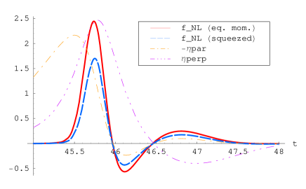
Figure 1: The non-Gaussianity parameter ${\tilde{f}}_{\mathrm{NL}}$ (36) for the two momentum configurations described in the text together with the slow-roll parameters $-\eta^{\parallel}$ and $\eta^{\perp}$, plotted as a function of time in the model (35) with initial conditions $\phi_{1}=\phi_{2}=13\kappa^{-1}$ and mass ratio $m_{2}/m_{1}=12$.

In figure 1 we show the result for the non-Gaussianity parameter ${\tilde{f}}_{\mathrm{NL}}$, defined as mf

$${\tilde{f}}_{\mathrm{NL}}\equiv\frac{\langle{\tilde{\alpha}}{\tilde{\alpha}}{\tilde{\alpha}}\rangle(k_{1},k_{2},k_{3})}{\left[\langle{\tilde{\alpha}}{\tilde{\alpha}}\rangle_{k_{1}}\langle{\tilde{\alpha}}{\tilde{\alpha}}\rangle_{k_{2}}+(k_{2}\leftrightarrow k_{3})+(k_{1}\leftrightarrow k_{3})\right]/3}$$ (36)

[where the $(2\pi)^{3}$ and the $\delta$-function are removed from the expression for the bispectrum], in the case of a mass ratio $m_{2}/m_{1}=12$. It is plotted as a function of time during the few e-folds of the corner-turning in field space, together with $\eta^{\parallel}$ and $\eta^{\perp}$. We show the results for two momentum configurations: (a) all three momenta equal, with horizon crossing 60 e-folds before the end of inflation, and (b) two momenta equal, crossing the horizon 60 e-folds before the end of inflation, with the third momentum crossing the horizon 20 e-folds earlier (squeezed configuration). We see that a large ${\tilde{f}}_{\mathrm{NL}}$ is produced initially but, in this model, is completely erased by the time $\eta^{\perp}$ has its first zero. The dependence on different momentum configurations can be inferred from (19) and (21). The main momentum dependence is the overall factor of $k^{-3/2}$ of $v_{am}^{(1)}$; however, if other momentum dependence were absent, these factors would cancel exactly in the definition of ${\tilde{f}}_{\mathrm{NL}}$. The remaining dependence on scale comes from the slow-roll suppressed dependence of $X_{am}$ on time and the fact that $\dot{{\mathcal{W}}}(k,t)$ peaks at different times for different modes. Because of this slow-roll suppression the momentum dependence is rather weak; figure 1 shows a variation of less than a factor 2 between two very different configurations.

The large non-Gaussianity of the type described above might be accessible in models where inflation ends during the corner-turning, such as hybrid inflation, or in which residual isocurvature modes persist. We have also investigated quartic potentials, and find that large, but temporary, non-Gaussianity emerges in a similar fashion. It may be that persistent large non-Gaussianity is easier to achieve in less symmetric potentials. Analytic calculations in RSvTnew , as well as further numerical investigations that are currently underway, should settle these issues.

VI Discussion

In this paper we extended and improved the non-Gaussian formalism developed in our earlier work. We derived and made use of a long-wavelength constraint relation (9), which simplifies the system of equations derived in mf ; formalism . We also clarified the issue of different time slicings at second order in order to properly connect to scalar observables. Using this formalism we have provided a general, exact expression for the bispectrum in multifield inflation due to superhorizon effects, equations (32)–(34), which provides a powerful way to compute non-Gaussianity for an arbitrary inflationary model up to the end of inflation. The computation is technically straightforward since it only requires the background solution and the linear perturbation solution at horizon crossing to be known, either analytically or numerically.

A numerical investigation of the simplest two-field quadratic example showed that non-Gaussianity can become large, as parametrized by a value of ${\tilde{f}}_{\mathrm{NL}}$ of order unity, whereas single-field inflation generically predicts a result two orders of magnitude smaller maldacena . In this model a temporary breakdown of slow roll is required somewhere during the last 40–50 e-folds of inflation (i.e. some time after the observable scales have left the horizon so that the scalar spectral index will not be too far from unity). This happens for mass ratios larger than about $10$ when the trajectory of the scalar fields driving inflation turns a corner, as parametrized by $\eta^{\perp}$. The large non-Gaussianity is produced by the nonlinear influence of the isocurvature mode on the adiabatic mode but it also decays away as the isocurvature mode disappears. The exact behaviour of ${\tilde{f}}_{\mathrm{NL}}$ as a function of time during inflation is complicated by subtle cancellations and a full explanation is left for a future publication RSvTnew . We find that there is only a weak dependence on the specific momentum configuration.

We note that earlier work in beruza emphasised the importance of the relation between non-Gaussianity and isocurvature modes, although their models relied on nonlinear interacting potentials to generate higher-order correlators. Related work in wandsvernizzi with the ‘$\delta N$’ formalism, using the same quadratic two-field potential, produced results which are qualitatively similar, that is, with large non-Gaussianity emerging temporarily. Numerically the $\delta N$ approach evolves neighbouring inflationary trajectories through a multidimensional field space, with appropriate derivatives estimated from these. In contrast, our approach relies more directly on integrals over the linear perturbation and background solutions which, in principle, should be more accurate. A direct quantitative comparison and an analysis of the relative merits of the two approaches deserves further investigation.

Attempts to incorporate inflation within the framework of a more fundamental physical theory like string theory or extensions of the Standard Model invariably lead to inflationary models with many scalar fields. Our findings indicate that non-Gaussianity can emerge naturally in these models, although its perdurance seems closely linked to that of the isocurvature modes. It is of great interest to investigate scenarios in which this non-Gaussianity might survive to late times because its imprint in the CMB may be observable in forthcoming experiments.

VII Acknowledgements

We are grateful for fruitful discussions with Neil Barnaby, Francis Bernardeau, James Cline, Jean-Philippe Uzan, Filippo Vernizzi, and David Wands. This research was supported by PPARC Grant No. PP/C501676/1.

References

- (1) G.I. Rigopoulos, E.P.S. Shellard, and B.J.W. van Tent, Phys. Rev. D73, 083522 (2006) [astro-ph/0506704].
- (2) G.I. Rigopoulos, E.P.S. Shellard, and B.J.W. van Tent, Phys. Rev. D73, 083521 (2006) [astro-ph/0504508]; G.I. Rigopoulos and E.P.S. Shellard, JCAP 10, 006 (2005) [astro-ph/0405185].
- (3) N. Bartolo, E. Komatsu, S. Matarrese, and A. Riotto, Phys. Rep. 402, 103 (2004) [astro-ph/0406398].
- (4) D.H. Lyth and Y. Rodriguez, Phys. Rev. Lett. 95, 121302 (2005) [astro-ph/0504045]; K. Enqvist and A. Vaihkonen, JCAP 09, 006 (2004) [hep-ph/0405103]; L.E. Allen, S. Gupta, and D. Wands, JCAP 01, 006 (2006) [astro-ph/0509719]; G. Calcagni, JCAP 10, 009 (2005) [astro-ph/0411773]; N. Bartolo, S. Matarrese, and A. Riotto, JCAP 08, 010 (2005) [astro-ph/0506410]; N. Barnaby and J. M. Cline, Phys. Rev. D73, 106012 (2006) [astro-ph/0601481].
- (5) F. Vernizzi and D. Wands, JCAP 05, 019 (2006) [astro-ph/0603799].
- (6) D. Langlois and F. Vernizzi, Phys. Rev. D72, 103501 (2005) [astro-ph/0509078]; D. Langlois and F. Vernizzi, JCAP 02, 017 (2007) [astro-ph/0610064].
- (7) S. Groot Nibbelink and B.J.W. van Tent, hep-ph/0011325 (2000).
- (8) S. Groot Nibbelink and B.J.W. van Tent, Class. Quantum Grav. 19, 613 (2002) [hep-ph/0107272]; B.J.W. van Tent, Ph.D. thesis (Utrecht University, 2002), available online at http://igitur-archive.library.uu.nl/dissertations/2002-1004-084000/inhoud.htm.
- (9) C. Gordon, D. Wands, B.A. Bassett, and R. Maartens, Phys. Rev. D63, 023506 (2001) [astro-ph/0009131].
- (10) G.I. Rigopoulos and E.P.S. Shellard, Phys. Rev. D68, 123518 (2003) [astro-ph/0306620].
- (11) V.F. Mukhanov, H.A. Feldman, and R.H. Brandenberger, Phys. Rep. 215, 203 (1992).
- (12) D. Seery and J.E. Lidsey, JCAP 09, 011 (2005) [astro-ph/0506056].
- (13) S. Weinberg, Phys. Rev. D72, 043514 (2005) [hep-th/0506236]; S. Weinberg, Phys. Rev. D74, 023508 (2006) [hep-th/0605244].
- (14) G.I. Rigopoulos, E.P.S. Shellard, and B.J.W. van Tent, in preparation.
- (15) J. Maldacena, JHEP 05, 013 (2003) [astro-ph/0210603]; V. Acquaviva, N. Bartolo, S. Matarrese, and A. Riotto, Nucl. Phys. B667, 119 (2003) [astro-ph/0209156]; G.I. Rigopoulos, E.P.S. Shellard, and B.J.W. van Tent, Phys. Rev. D72, 083507 (2005) [astro-ph/0410486].
- (16) F. Bernardeau and J.-P. Uzan, Phys. Rev. D66, 103506 (2002) [hep-ph/0207295]; F. Bernardeau and J.-P. Uzan, Phys. Rev. D67, 121301 (2003) [astro-ph/0209330].