Supernova limits on brane world cosmology

Abstract

By combining the first year data from the Supernova Legacy Survey (SN LS) and the recent detection of the baryon acoustic peak in the Sloan Digital Sky Survey data, we are able to place strong constraints on models where the cosmic acceleration is due to the leakage of gravity from the brane into the bulk on large scales. In particular, we are able to show that the DGP model is not compatible with a spatially flat universe. We generalize our analysis to phenomenological toy models where the curvature of the brane enters into the Friedmann equations in different ways.

,

1 Introduction

Observations of Type Ia supernovae have led us to understand that the universe started to accelerate at a redshift of $z\sim 1$ [1, 2, 3, 4]. This suggests the presence of some energy component which redshifts slowly and which had the same density as matter relatively recently, $z<1$. The desire to explain this behaviour has led to the development of a number of models such as quintessence where the energy density corresponds to the potential energy of some scalar field.

At the same time, models with large extra dimensions into which only gravity can propagate have become popular which suggests that there may be short distance corrections to gravity [5, 6]. When the Friedmann equations are solved in these higher dimensional backgrounds, the expression for the Hubble parameter changes to $H^{2}=G(\rho+k\rho^{2})$ where $k$ is related to the tension of the brane upon which the standard model particles reside [7]. However, modifications of this form do not give rise to the kind of behaviour required to explain the observed acceleration.

A related theory is that due to Dvali, Gabadadze and Porrati (DGP), which presents a class of brane theories where the theory remains four dimensional at short distances but crosses over to a higher dimensional theory for gravity at some very large distance [8]. In this model, gravity leaks out into the bulk only at large distances and the resulting modifications to the Friedmann equations can give rise to universes with acceleration [9, 10].

In section 2 we will briefly present the DGP model and then we will show in section 3 that is it marginally disfavoured by observations of supernovae and baryon oscillations, at least in the case of a spatially flat universe. In section 4 we will try to generalise the 1st (tt) Friedmann equation obtained in the DGP model to see if the data indicates what kinds of modifications to the Friedmann equations might explain the data.

2 The DGP model

The DGP theory starts with the idea that standard model gauge fields are confined to live on a (3+1)D brane residing in an infinite (4+1)D bulk, with different scales of gravity on the brane and in the bulk [8]. The gravitational part of the action is therefore given by

$$S=\frac{1}{2\mu^{2}}\int d^{5}z\sqrt{-g_{5}}R_{5}+\frac{1}{2\kappa^{2}}\int d^{4}x\sqrt{-g_{4}}R_{4}$$ (1)

where $\mu^{2}=M_{Pl}^{-2}$ and $\kappa^{2}=M_{5}^{-3}$. The Friedmann equation which comes from this gravitational action coupled to matter on the brane take the form [11]

$$\epsilon\sqrt{H^{2}+\frac{k}{a^{2}}}=\frac{\kappa^{2}}{2\mu^{2}}\left(H^{2}+\frac{k}{a^{2}}\right)-\frac{\kappa^{2}}{6}\rho$$ (2)

where $\epsilon=\pm 1$. For our purposes it is important to note at this point that the corrections to the normal equations involve the extrinsic curvature of the brane itself, in other words $H^{2}+ka^{-2}$. Later when we try and generalise this equation to compare with the data, this observation will loosely motivate the form of our generalisation. If we set $\epsilon=1$ we can re-arrange things so that the Friedmann equation takes the form

$$H^{2}+\frac{k}{a^{2}}=\left(\sqrt{\frac{\rho}{3M_{Pl}^{2}}+\frac{1}{4r_{c}^{2}}}+\frac{1}{2r_{c}}\right)^{2}$$ (3)

where the length scale $r_{c}$ is defined to be

$$\frac{1}{2r_{c}}=\frac{\mu^{2}}{\kappa^{2}}$$ (4)

and $r_{c}$ sets a length beyond which gravity starts to leak out into the bulk, modifying the Friedmann equations. The relationship between the Hubble expansion parameter today $H_{0}$ and that at a redshift $z$ is then given by

$$\frac{H(z)^{2}}{H_{0}^{2}}=H^{\prime}(z)^{2}=\Omega_{k}(1+z)^{2}+\left(\sqrt{\Omega_{M}(1+z)^{3}+\Omega_{r_{c}}}+\sqrt{\Omega_{r_{c}}}\right)^{2}$$ (5)

where we use the usual notation $\Omega_{x}=\rho_{x}/\rho_{crit}$ where $\rho_{x}$ refers to the energy density in component $x$ today and $\rho_{crit}=3H_{0}^{2}/8\pi G$. The new unusual parameter $\Omega_{r_{c}}$ takes the form

$$\Omega_{r_{c}}=\frac{\mu^{4}}{\kappa^{4}H_{0}^{2}}$$ (6)

and the constraint equation between the various components of energy density at $z=0$ is given by

$$\Omega_{M}+\Omega_{k}+2\sqrt{\Omega_{r_{c}}}\sqrt{1-\Omega_{k}}=1$$ (7)

So that, in particular for a flat universe with $k=0$ we have the relation

$$\Omega_{r_{c}}=\frac{(1-\Omega_{M})^{2}}{4}$$ (8)

It has been shown that by setting the length scale $r_{c}$ close to the horizon size, this extra contribution to the Friedmann equation leads to acceleration which can in principle explain the supernova data [9, 10]. In the next section we will see if this theory can fit with the latest observations.

3 Confronting the model with cosmological data

Measurements of the brightness of Type Ia supernovae as a function of redshift are sensitive to the cosmological model via the integration over expansion history in the expression for the luminosity distance ($c=1$)

$$d_{L}=\frac{1+z}{H_{0}\sqrt{|\Omega_{k}|}}{\cal S}\left(\sqrt{|\Omega_{k}|}\int_{0}^{z}{{d\tilde{z}\over H^{\prime}(\tilde{z})}}\right)$$ (9)

where the function ${\cal S}(x)$ is defined as $\sin(x)$ for $\Omega_{k}<0$ (closed Universe), $\sinh(x)$ for $\Omega_{k}>0$ (open Universe) and ${\cal S}(x)=x$, and the factor $\sqrt{|\Omega_{k}|}$ is removed for the flat Universe

In the DGP model, $H(z)$ is then given by Eq.(5). Very recently, the SNLS collaboration published the first ear data of its planned five year survey (Astier et al, 2005) [12]. The data set includes 71 high redshift Type Ia supernovae (SNIa) in the redshift range z=[0.2,1] and 44 low redshift SNIa compiled from the literature but analysed in the same manner as the high-z sample. Thanks to the multi-band, rolling search technique and careful calibration, this data-set is arguably the best high-z SNIa compilation to date, indicated by the very tight scatter around the best fit in the Hubble diagram and the careful estimate of systematic uncertainties in [12]. In our analysis (as in [12]) we fit for cosmological parameters with the prior from the baryon oscillation peak detected in the SDSS Luminous Red Galaxy survey (LRG) of Eisenstein el al (2005) [13], given by

$${\sqrt{\Omega_{M}}\over E(z_{1})^{1\over 3}}\left[{1\over z_{1}\sqrt{|\Omega_{k}|}}{\cal S}\left(\sqrt{|\Omega_{k}|}\int_{0}^{z_{1}}{dz\over E(z)}\right)\right]^{2\over 3}=0.469\pm 0.017,$$ (10)

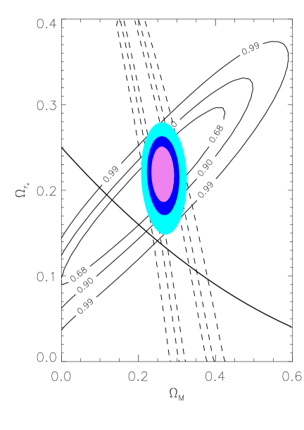
where $E(z)=H(z)/H_{0}$ and $z_{1}=0.35$. Furthermore, ${\cal S}$ and $\Omega_{k}$ are defined as in Eq.(9). The quoted uncertainty corresponds to one standard deviation, where a Gaussian probability distribution has been assumed. Figure 1 shows the allowed regions in the $\Omega_{r_{c}}$–$\Omega_{M}$ plane in the DGP model from each of the two data sets and the combined limits. Also shown in the graph is the curve corresponding to flatness, i.e. $\Omega_{k}=0$.

The allowed region of the $\Omega_{r_{c}}$–$\Omega_{M}$ plane deduced from baryon oscillations forms a band whereas the allowed region from supernovae luminosity measurements forms an ellipsoid. The fact that the baryon oscillations constrain models to lie on a band reflects the fact that they have only so far been detected at two redshifts, $z=0.35$ in the SDSS data and $z\sim 1100$ in the CMB data. This gives us one ratio vs. the many ratios which come from the many type 1a supernovae. However, the power of this approach lies in the fact that the band of allowed parameters from baryon oscillations is almost perpendicular to the major axis of the ellipsoid coming from the supernovae data. This occurs in a very similar way in the conventional $\Omega_{\Lambda}$–$\Omega_{M}$ plane. The use of the baryon oscillation prior therefore allows us to constrain model universes much more effectively.

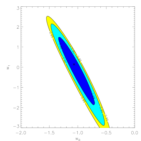
We conclude that the fit of the DGP model to the supernova data along with a prior from the baryon oscillation results is incompatible with a flat universe. Given the evidence for the latter from the CMB experiments, this model is clearly disfavoured by the current observational data. For comparison, in Figure2 we show the fit to the same data to a dark energy model generically described by an equation of state parameter, $w(z)=w_{0}+w_{1}\cdot z$, where a flat universe is assumed. The $\Lambda$ model $(w_{0}=-1,w_{1}=0)$ gives an excellent fit to the data. All the fits were performed with a modified version of the cosmology fitter (SNALYS) in the SNOC package [14].

Figure 1: The solid curves show the allowed parameter regions in the $\Omega_{M}-\Omega_{r_{c}}$ plane at the 68, 90 and 99% confidence level. Solid thin contours correspond to the the first year SNLS data in Astier et al (2005)[12], the dashed lines show the corresponding regions from the baryon oscillation peak in Eisenstein et al (2005) [13]. The coloured contours indicate the result of the combination of both data-sets. The thick solid lines indicate the expected relation between $\Omega_{M}$ and $\Omega_{r_{c}}$ in a flat universe.

Figure 2: Allowed 68, 90 and 95 % confidence regions in the $w_{0}$,$w_{1}$ parameter space for the first year SNLS data with baryon oscillation prior in a flat universe. The linear expansion $w(z)=w_{0}+w_{1}\cdot z$ has been assumed. The best fit solution $(w_{0}=-1.07,w_{1}=0.14)$ is also shown.

4 Generalisations of the DGP model

We would like to consider generalisations of the DGP model in order to see if the data favours any particular modification of the Friedmann equation. (This is in the spirit of [15] and [16].) The extra term in the Friedmann equation (2) comes from the derivative of the scale factor in the 5th dimension, which is set by the Israel branching conditions across the brane and therefore by the extrinsic curvature on the brane. We will therefore assume the extra term enters in the following form

$$\left(H^{2}+\frac{k}{a^{2}}\right)^{\alpha/2}=\frac{\kappa_{*}^{2}}{2\mu^{2}}\left(H^{2}+\frac{k}{a^{2}}\right)-\frac{\kappa_{*}^{2}}{6}\rho_{m}$$ (11)

where now $\alpha$ is a free parameter and $\kappa_{*}^{2}$ is now related to some phenomenological mass scale $\tilde{M}$

$$\kappa_{*}^{2}=\tilde{M}^{\alpha-4}.$$ (12)

The expression for the Hubble expansion as a function of redshift is then

$$\frac{H(z)^{2}}{H_{0}^{2}}+\frac{k}{a^{2}H_{0}^{2}}-\frac{2\mu^{2}}{\kappa_{*}^{2}H_{0}^{2-\alpha}}\left(\frac{H(z)^{2}}{H_{0}^{2}}+\frac{k}{a^{2}H_{0}^{2}}\right)^{\alpha/2}=\Omega_{M}(1+z)^{3}$$ (13)

or equivalently

$$\frac{H(z)^{2}}{H_{0}^{2}}-\Omega_{k}(1+z)^{2}-2\sqrt{\Omega_{r_{c}}}\left(\frac{H(z)^{2}}{H_{0}^{2}}-\Omega_{k}(1+z)^{2}\right)^{\alpha/2}=\Omega_{M}(1+z)^{3}$$ (14)

where now we have generalised the expression for the DGP brane world dark energy density fraction

$$\sqrt{\Omega_{r_{c}}}=\frac{\mu^{2}}{\kappa_{*}^{2}H_{0}^{2-\alpha}}$$ (15)

which means that the constraint between the various densities at $z=0$ is given by

$$\Omega_{M}+\Omega_{k}+2\sqrt{\Omega_{r_{c}}}(1-\Omega_{k})^{\alpha/2}=1$$ (16)

In order to make sure there are no pathologies here, we need to ensure that

$$\Omega_{k}<1-\Omega_{M}\qquad;\qquad(\Omega_{M}>0)$$ (17)

then if we write

$$h=\sqrt{\frac{H(z)^{2}}{H_{0}^{2}}+\frac{k}{a^{2}H_{0}^{2}}}$$ (18)

we can then solve the following equation as a function of redshift

$$h^{2}-2\sqrt{\Omega_{r_{c}}}h^{\alpha}=\Omega_{M}(1+z)^{3}$$ (19)

and use the solution to obtain the luminosity distance. Since $\alpha$ is no longer $\alpha=1$ we now obtain the solutions to this equation numerically.

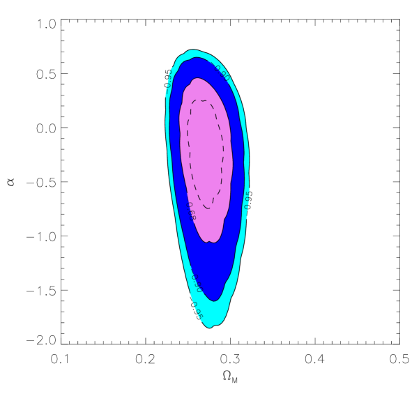
Figure 3 shows the allowed values in the $\alpha$–$\Omega_{M}$ parameter space if a flat universe prior is imposed. The best fits are centered close to $\alpha=0$, which corresponds to a constant in Eq.(14), i.e. equivalent to $\Lambda$. The full data set of the SNLS, $\sim$700 spectroscopically confirmed Type Ia SNe, will soon provide further constraints in the possible values of the exponent $\alpha$.

Figure 3: Allowed parameter regions in the $\alpha$–$\Omega_{M}$ plane at the 1 $\sigma$ (one parameter), 68, 90 and 95% confidence level for a flat universe.

5 Conclusions

The most recent high-redshift supernova data has been used to test the DGP brane model of cosmology where dark energy is replaced by an extension of the Friedmann equation to account for the leakage of gravity to a large extra dimension. Using a prior from the SDSS baryon oscillation results we find that the this model is incompatible with the data for a flat universe. Generalizations of the model including an extra term $H^{\alpha}/r_{c}^{2-\alpha}$ yields $-0.8<\alpha<0.3$ (1 $\sigma$) i.e consistent with $\alpha=0$, the situation corresponding to a non-redshifting cosmological constant.

This is not completely surprising if we look at the generalised Friedmann equation (11) since during the matter dominated era, it is straightforward to show that the equation of state $w=-1+{\alpha\over 2}$ [15]. Observational constraints on $w$ already push us close to $w\sim-1$ (see Figure 2) so we see that we require some small value of $\alpha$ in order to match the observations at this time.

Finally, we note that it may be interesting in the future to see if it is possible to obtain a good fit to the data in models which give rise to different modifications to the Friedmann equations.