External Sources of Poynting Flux in MHD Simulations of Black Hole Ergospheres

Abstract

This article investigates the physics that is responsible for creating the outgoing Poynting flux emanating from the ergosphere of a rotating black hole in the limit that the magnetic energy density greatly exceeds the plasma rest mass density (magnetically dominated limit). The underlying physics is derived from published 3-D simulations that obey the general relativistic equations of perfect magnetohydrodynamics (MHD). It is found that the majority of the outgoing radial Poynting flux emitted from the magnetically dominated regions of the ergosphere is injected into the magnetosphere by a source outside of the event horizon. It is concluded that the primary source of the Poynting flux is associated with inertial forces in the magnetically dominated region proper or in the lateral boundaries of the region. However, the existing numerical data does not rule out the possibility that large computational errors are actually the primary source of the Poynting flux.

There are two known theoretical mechanism for producing field-aligned outgoing poloidal Poynting flux, $S^{P}$, at the expense of the rotational energy of a black hole in a magnetosphere that is magnetically dominated. There are electrodynamic processes collectively called Blandford-Znajek mechanisms in which currents flow virtually parallel to the proper magnetic field direction (force-free currents) throughout the magnetically dominated zone all the way to the event horizon Blandford and Znajek (1977); Phinney (1983); Thorne et al (1986). Therefore, these electrodynamic currents have no source within the magnetically dominated black hole magnetosphere. Alternatively, there is the GHM (gravitohydromagnetic) dynamo in which large relativistic inertia is imparted to the tenuous plasma by black hole gravity that in turn creates a region of strong cross-field currents (inertial currents), $J^{\perp}$, that provide the source of the field-aligned poloidal currents, $J^{P}$ supporting $S^{P}$ in an essentially force-free outgoing wind (see Punsly (2001) or the seminal articles Punsly and Coroniti (1990); Punsly (1991)). The force-free electrodynamic current flow is defined in terms of the Faraday tensor and the current density as $F^{\mu\nu}J_{\nu}=0$. As a consequence, $\mathbf{J}\cdot\mathbf{E}=0$, so $S^{P}$ in a force-free magnetosphere must be injected from a boundary surface. The two types of sources associated with these two types of Poynting fluxes are quite distinct in the ergopshere: $J^{\perp}$ provides the $\mathbf{J}\cdot\mathbf{E}$ source in Poynting’s Theorem and the force-free (electrodynamic) component of $S^{P}$ emerges from a boundary source at the event horizon.

Numerical models can be useful tools for understanding the source of $S^{P}$ emerging from the ergosphere of a black hole magnetosphere. Some recent 3-D simulations in De Villiers et al (2003); Hirose et al (2004); De Villiers et al (2005a, b); Krolik et al (2005) show $S^{P}$ emanating from magnetically dominated funnels inside of the vortices of thick accretion flows. In these simulations, $J^{\perp}\approx J^{\theta}$(in Boyer-Lindquist coordinates which are used throughout the following) inside of the ergosphere, since the poloidal field settles to a nearly radial configuration early on in the simulation Hirose et al (2004). In principle, one can clearly distinguish the amount of $S^{P}$ emerging from the ergosphere in a simulation that is of electrodynamic origin (as proposed in Blandford and Znajek (1977)) from the amount due inertial effects (the GHM theory of Punsly (2001)) by quantifying the relative strengths of $S^{P}$ emerging from the inner boundary (the asymptotic space-time near the event horizon) with the amount created by sources within the ergosphere. In the high spin rate simulations in questions, over 72% of $S^{P}$ emerging from the ergopsheric funnel is created outside of the inner boundary.

The simulation that is analyzed, ”KDE” is one of a family of solutions described in De Villiers et al (2003); Hirose et al (2004); De Villiers et al (2005a, b); Krolik et al (2005). The solutions within the family can be distinguished by their spin rate as defined by the ratio of black hole angular momentum to mass, $a/M$. The KDE simulation spins the most rapidly with, $a/M=0.998$. All of the simulations begin with a torus surrounding the black hole which would be stable if not for the ad hoc introduction of loops of poloidal magnetic field along the equal pressure contours. This destabilizes the torus as the shearing of the loops in the differentially rotating plasma creates magnetic torques on the plasma that initiates an accretion flow. The angular momentum removal by the field is sustained by the inward flow of gas that approaches a centrifugal barrier near the black hole. This barrier creates an ”inner edge” of the accretion flow that forms a funnel roughly along the gravitational equipotential surface. The subsequent accretion of gas is restricted primarily to the equatorial plane. As the magnetic flux loops accrete, the upper portion gets stretched vertically by gas pressure gradients and electromagnetic forces forces away from the hole and the inward part of the loop gets severely twisted azimuthally as it approaches the horizon. The field lines become inextricably tangled. The net result is the formation of magnetic field lines that are approximately radial, but highly twisted azimuthally, in the region near the black hole, restricted to the funnel.

The KDE solution with $a/M=0.998$ has by far the most powerful outward Poynting flux in the funnel within in the family of simulations. It is the only solution in which this energy flux is comparable with the energy flux emerging in a mildly relativistic jet created within the funnel wall (the boundary or shear layer between accretion disk and the funnel). The KDE simulation is the only one that appears capable of supplying the high power relativistic jets that are observed in kinetically dominated FRII quasars (the kinetic luminosity equals or exceeds the bolometric luminosity of the accretion flow). As an example in Cygnus A and 3C 82, the jet kinetic luminosity is roughly 5-10 times the bolometric luminosity of the thermal emission from the accretion flow (see the supplementary material in Semenov et al (2004)). Consequently, from an astrophysical perspective the KDE simulation is very intriguing.

Ostensibly, one might think that the spin rate of $a/M=0.998$ is a benign change from the KDP simulation in De Villiers et al (2003); Hirose et al (2004); De Villiers et al (2005a, b); Krolik et al (2005) with $a/M=0.9$. A significant difference is that the surface area of the equatorial plane in the the ergopshere (the active region of the black hole) is almost 2.5 times larger in the $a/M=0.998$ case Punsly (2001); Semenov et al (2004).

The paper is organized as follows. Section 1 introduces notation and basic concepts that describe MHD black hole magnetospheres. This is not new material, but it is taken from existing literature and provides a framework for the discussion to follow. The second section presents Poynting’s theorem in curved space-time in integral form, the energy conservation equation for the electromagnetic field. The primary result of this section appears in section 2.3: over 72% of $S^{P}$ emerging from the ergopsheric funnel during the course of the simulation is created outside of the inner boundary. This result follows directly from the data presented in Krolik et al (2005) and does not require any interpretation or manipulation of the data. In order to verify that the data sampled is faithful to the simulation in Krolik et al (2005), we note an independent result from the same work in section 2.4: there is also a strong source of field aligned poloidal angular momentum flux, $S_{L}^{P}$ in the ergosphere. The source of $S_{L}^{P}$ is co-spatial with the source of $S^{P}$ and of similar magnitude, i.e., over 70% of $S_{L}^{P}$ that emerges from the ergosphere is created external to the event horizon. This means that either the simulation truly has an electromagnetic source in the ergosphere or there are two independent plots in Krolik et al (2005) that have coincidental errors. In section 3, it is shown that there is a unique physical explanation of the source of $S^{P}$ and $S_{L}^{P}$ that is consistent with Faraday’s law averaged over time and azimuth (the sampled data from the simulation is averaged over time and azimuth in Krolik et al (2005)). A physically acceptable source must be a cross-field poloidal current (inertial current, since it is associated with strong $\mathbf{J}\times\mathbf{B}$ forces in the momentum equation of the plasma). By Ampere’s law this current supports a toroidal magnetic field that is the field component required for a jump in both $S^{P}$ and $S_{L}^{P}$ (averaged over time and azimuth) in the ergosphere. The GHM theory of black hole magnetospheres is based on such a current. The only thing that would invalidate this straightforward calculation are significant numerical errors in the simulation. Section 3 is the only section in this paper that manipulates the data in Krolik et al (2005) and so it does not carry the same weight as the direct results of section 2. However, the analysis of section 3 is useful (even if it turns out to be misleading) for the development of future simulations because such an outcome would indicate gross inconsistencies within the data in Krolik et al (2005). Section 4 compares the results seen in KDE with other simulations of rotating black hole magnetospheres. This motivates a discussion in the section 5 of the various numerical techniques and why they tend to either support or not support the KDE simulation, in particular the differences with the simulations in McKinney and Gammie (2004); McKinney (2005) are highlighted. Possible sources of numerical error are explored in terms of computational technique and coordinate systems. There is also a discussion of the need for 3-D simulations versus 2-D simulations. In the conclusion, we stress the need for further simulations to see if this is indeed a valid interpretation of the data. Some suggestions on how future data should be sampled are offered. Key parameters to monitor are mentioned and likely candidates for numerical artifacts are noted as a guide to help future efforts sort out this complicated turbulent problem.

1 Physical Quantities in Boyer-Lindquist Coordinates

The Kerr metric (that of a rotating uncharged black hole), $g_{\mu\nu}$, in Boyer-Lindquist coordinates $(r,\theta,\phi,t)$, is given by a line element that is parameterized by the black hole mass, $M$, and the angular momentum per unit mass, $a$, in geometrized units Thorne et al (1986). We use the standard definitions, $\rho^{2}=r^{2}+a^{2}\cos^{2}\theta$ and $\Delta=r^{2}-2Mr+a^{2}$, where $\Delta=0$ at the event horizon, $r_{{}_{+}}=M+\sqrt{M^{2}-a^{2}}$. The ”active” region of space-time is the ergosphere, where black hole energy can be extracted, $r_{{}_{+}}<r<r_{s}=M+\sqrt{M^{2}-a^{2}\cos^{2}\theta}$ Penrose (1969).

The flux of electromagnetic angular momentum along the poloidal magnetic field direction is the component of the stress-energy tensor, $T_{\phi}^{\;r}=[1/(4\pi)]F_{\phi\alpha}F^{\alpha r}$, in the approximation that the field is radial. In steady state, the electromagnetic angular momentum flux per unit poloidal magnetic flux is the toroidal magnetic field density: $-B^{T}\equiv\sqrt{-g}\,F^{\theta r}$, where $g=-\rho^{4}\sin^{2}{\theta}$ Phinney (1983); Punsly (2001). Similarly, the electromagnetic energy flux along the poloidal magnetic field direction, $S^{P}$, is the component, $T_{t}^{\;r}=[1/(4\pi)]F_{t\alpha}F^{\alpha r}$, in the approximation that the poloidal field is radial Thorne et al (1986). In steady state, the energy flux per unit poloidal magnetic flux is $-(\Omega_{{}_{F}}/c)B^{T}$, where $\Omega_{{}_{F}}$ is the field line angular velocity Phinney (1983); Punsly (2001). Consequently, $B^{T}$ is useful for quantifying the energy and angular momentum fluxes as steady state is approached. From Ampere’s law,

$$\sqrt{-g}\frac{4\pi}{c}J^{\theta}=B^{T}_{\;\;,r}+(\sqrt{-g}F^{\theta\phi})_{,\phi}+(\sqrt{-g}F^{\theta t})_{,t}\;,$$ (1)

evaluated at late times (as an approximate steady state is reached), one expects simulation data that is averaged over azimuth to obey $\sqrt{-g}J^{\theta}\approx B^{T}_{\;\;,r}$. Therefore, at late times, $J^{\theta}$ is a potential source for the current system that supports $S^{P}$.

Even when a system has not reached a time stationary state, one can introduce a well-defined notion of $\Omega_{{}_{F}}$ that becomes the field line angular velocity in the steady state. If the field is nearly radial one can simply define the expression, $F_{t\theta}\equiv-\Omega_{{}_{F}}F_{\theta\phi}$. With this definition, $\Omega_{{}_{F}}$ is a function of space and time and in steady state it becomes a constant along a perfect MHD flux tube Phinney (1983). Therefore, the EMF across the magnetic field is $-\Omega_{{}_{F}}F_{\theta\phi}$ by definition.

2 The Source of Ergospheric Poynting Flux in the KDE Simulation

The simulation ”KDE” of De Villiers et al (2003); Hirose et al (2004); De Villiers et al (2005a, b); Krolik et al (2005) is of the most interest since it generates an order of magnitude more $S^{P}$ than any of the other simulations Krolik et al (2005). The magnetically dominated funnel spans the latitudes $0^{\circ}<\theta<55^{\circ}$ at the inner calculational boundary, near $r_{{}_{+}}$. Quantifying the magnetic dominance in the funnel is the pure Alfven speed, $U_{A}=B^{P}/(\sqrt{4\pi n\mu}c)$, where $n$ is the proper number density, $\mu$ is the specific enthalpy of the plasma and $B^{P}$ is the poloidal field strength: within the funnel, $10<U_{A}^{2}<10^{4}$.

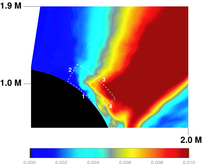
Figure 1: The azimuthally averaged and time averaged (over 75% of the simulation that ends at $t=8080M$) Poynting flux from the model KDE ($a/M=0.998$) of Krolik et al (2005). The figure is a magnification of the inner region of figure 10 of Krolik et al (2005). It is an excision of a region, $0^{\circ}<\theta<65^{\circ},r\sim r_{+}$ that is a little larger than the ergospheric portion of the magnetically dominated funnel, $0^{\circ}<\theta<55^{\circ},r\sim r_{+}$. The majority of $S^{P}$ switches-off in a thin layer near $r=1.3M$ - $r=1.5M$ (see Krolik et al (2005) for a description of the units on the color bar). A Gaussian pillbox, $30^{\circ}<\theta<55^{\circ}$, is drawn as a dashed white contour for use in Poynting’s Theorem. There are 26 grid zones between the inner boundary, $r=1.175M$ and $r=1.5M$. The plot is provided courtesy of John Hawley.

2.1 Poynting’s Theorem

The source of $S^{P}$ can be determined from the integral version of Poynting’s Theorem, which is the integral of $T^{\nu}_{t\;\;;\nu}=F_{t\nu}J^{\nu}$ combined with Stokes’ theorem. In Boyer-Lindquist coordinates, the curved space-time equivalent of the ”$\mathbf{J}\cdot\mathbf{E}$” source of $S^{P}$ is $F_{t\alpha}J^{\alpha}$. In steady state, the source of $S^{P}$ is $-\Omega_{{}_{F}}F_{\theta\phi}J^{\theta}$ in the approximation of a radial field. Without the radial approximation, one needs to define a poloidal field direction, $\mathbf{B^{P}}$, and a cross-field poloidal EMF, $E_{\perp}\equiv-\Omega_{{}_{F}}B^{P}$ then the source of $S^{P}$ is $E_{\perp}J^{\perp}$. This can all be setup with great mathematically complexity (see Punsly (2001) for sample calculations) and no additional physical insight. The reader should remember that the poloidal field is not exactly radial in the following and the simple notion of $J^{\theta}$ is used to approximate $J^{\perp}$.

The funnel is highly turbulent and even averaging over $\phi$ does not damp the large field strength variations that are seen in snapshots of this rotating non-axisymmetric system (DeVilliers privative communication 2005). Finding a source of Poynting flux in a time snapshot is futile since the field strength variability manifests itself as large fluctuations in the Poynting flux on the inner calculational boundary near the horizon and throughout the ergosphere (Hawley private communication 2005). Conversely, over long periods of time the total outflow of energy swamps the local random turbulent behavior seen in any time snapshot. For this reason Krolik et al (2005) time averaged all the data in order to extricate the persistent physics from the strong turbulent fluctuations that obscure the physics in individual snapshots. In order to understand the source, one is interested in where the total time integrated Poynting flux that radiates from the ergosphere originates. This information can be obtained by performing a time integral of the simulation, once the large transients have died down. The discrete time average and azimuthal average of $S^{P}$ in the KDE simulation near $r_{{}_{+}}$ is shown in figure 1. The time integral of $S^{P}$ can be approximated by multiplying the discrete time average by the total time. The contour map in figure 1 indicates a region of strong outgoing $S^{P}$ in the evacuated funnel, $30^{\circ}<\theta<55^{\circ}$, $r\sim r_{+}$. It is clear that $S^{P}$ suddenly diminishes close to $r_{+}$ at $r\approx 1.3M-1.5M$.

In order to investigate possible source terms for $S^{P}$, one needs to be explicit about what is plotted in figure 1. The data was averaged over $\phi$ and $t$ (denoted by ”$<>$”). Whenever a time lapse of 80 M occurs within the high time resolution simulation, data was stored for a time ”snapshot”. There are 76 of these snapshots that are averaged in figure 1, steps 26 through 101. Thus, the discrete time average of Poynting’s theorem is relevant to figure 1,

$$[2/\pi]\frac{1}{76}\sum_{i=26}^{101}\left[\int[F_{t\phi}J^{\phi}+F_{tr}J^{r}+F_{t\theta}J^{\theta}]\,dV\right]_{i}$$

$$-[2/\pi]\frac{1}{76}\sum_{i=26}^{101}\left[\frac{d}{dt}\int T^{\,t}_{t}\,dV\right]_{i}$$

$$=[1/(2\pi^{2})]\frac{1}{76}\sum_{i=26}^{101}\left[\int_{1+3}\sqrt{-g}F_{t\alpha}F^{\alpha r}\,d\theta\,d\phi\right]_{i}$$

$$+[1/(2\pi^{2})]\frac{1}{76}\sum_{i=26}^{101}\left[\int_{2+4}\sqrt{-g}F_{t\alpha}F^{\alpha\theta}\,dr\,d\phi\right]_{i}\;,$$ (2)

where the four sides of the Gaussian pillbox of integration in figure 1 are the four curves labelled ”1 -4” and $dV=\sqrt{-g}drd\phi d\theta$ is the spatial volume element. Periodic boundary conditions are imposed at $\phi=0$ and $\phi=\pi/2$. Hence, $<T_{t}^{\;\phi}>$ is equal at both boundaries and does not contribute to surface integral on the RHS of (2).

2.2 Limitations of the Existing Data

The data that was stored in the run of the KDE simulation does not allow us to compute all of the terms in Poynting’s theorem, (2), in each of the coarse time steps, ”i”. For example, since at least three consecutive fine resolution time steps were not stored at each of the 76 coarse time steps, one can not compute the time derivative or the current density (from Ampere’s law) that appear in Poynting’s theorem. This highlights the limitation of single snapshot information. A computation of $T_{t\;;\nu}^{\,\nu}$ in a single noisy snapshot never includes the $d/dt(T^{t}_{\;t})$ which is likely to dominate in a turbulent environment, nor can one compute $J^{\mu}$. Thus, such a calculation is likely to be very misleading. For this reason the time averaged data presented in Krolik et al (2005) is considerably better. Even though $J^{\mu}$ can not be computed, one expects that the $d/dt(T_{t}^{\;t})$ term time averages to zero if the system is physical (i.e., a finite field energy density in a small spatial region should not decay as a persistent source of Poynting flux). Even so, we are limited by not being able to compute $\mathbf{J}\cdot\mathbf{E}$. However, there are conclusions that can be reached. First of all figure 1 can be used to compare the total $S^{P}$ radiated from $r_{{}_{+}}$ and $r_{s}$. This is the subject of section 2.3 and the results do not depend on any analysis of the data, but follow directly from the data. Secondly, we have time averaged information on $<T_{\phi}^{\;r}>$ from Krolik et al (2005) which allows us to restrict the source terms in (2). Using this information in section 3.3, we deduced that there is only one source that is consistent with the $<T_{\phi}^{\;r}>$ and the $<T_{t}^{\;r}>$ data from Krolik et al (2005), $<\mathbf{J}\cdot\mathbf{E}>$. However, without having the actual data, complete with differential information, one can not assess the level to which numerical errors invalidate the conclusions of section 3.3.

2.3 The Horizon is not the Primary Source of Poynting Flux

The total Poynting flux emanating from inner ergosphere, $r<1.5M$, after the large transients have died down, $2000M<t<8080M$, is $\approx(20/\pi)M\sum_{i=26}^{101}\int_{3}\sqrt{-g}F_{t\alpha}F^{\alpha r}\,d\theta\,d\phi$. Similarly, the time integrated $S^{P}$ emanating from inner boundary (horizon), after the large transients have died down, $2000M<t<8080M$, is $\approx(20/\pi)M\sum_{i=26}^{101}\int_{1}\sqrt{-g}F_{t\alpha}F^{\alpha r}\,d\theta\,d\phi$. The result of significance from this plot is that $\sum_{i=26}^{101}\int_{3}\sqrt{-g}F_{t\alpha}F^{\alpha r}\,d\theta\,d\phi>3.5\mid\sum_{i=26}^{101}\int_{1}\sqrt{-g}F_{t\alpha}F^{\alpha r}\,d\theta\,d\phi\mid$, i.e. $\int S^{P}\,dt$ emitted from the inner boundary (horizon) during the interval, $2000M<t<8080M$, is much smaller than $\int S^{P}\,dt$ emitted from $r_{s}$ during the interval, $2000M<t<8080M$. Because of the saturation of the dark red color in the plotting routine, $S^{P}$ might be even larger above the switch-off layer than indicated in the contour map. Thus, we only have a lower bound on the strength of $S^{P}$ above the switch-off layer and it is likely that more than 72% of the total $S^{P}$ is created within this thin layer. At this point, we can conclude that during the interval $2000M<t<8080M$, less than $28\%$ of $S^{P}$ that emerges from the ergospheric funnel came from the inner boundary, the rest was created external to the boundary.

2.4 The Ergospheric Source of Angular Momentum Flux

One could conjecture that without the actual data in hand that it might be difficult to assess whether the source seen in the false color and the embedded white contours in figure 1 truly reflects the simulation. Thus, we are compelled to find supporting data. First of all, is the external source a plotting routine artifact? Secondly, one might ask if there is any other supporting information that there is a strong electromagnetic source external to the horizon? Fortunately, there are a family of line plots of the electromagnetic angular momentum flux as a function of $\theta$ and $r$ in Figure 7 of Krolik et al (2005). Each line plot represents the averaged (in $t$ and $\phi$) electromagnetic angular momentum flux,

$$<T_{\phi}^{\;r}>=[1/(4\pi)][<F_{\phi t}F^{tr}>+<F_{\phi\theta}F^{\theta r}>]\;,$$ (3)

as a function of $\theta$ on a $r$=constant surface. Figure 7 shows that $<T_{\phi}^{\;r}>$ is created predominantly in the ergosphere, outside of the horizon. Over 70% of the electromagnetic angular momentum flux in the funnel is created by sources within the ergopshere for $25^{\circ}<\theta<55^{\circ}$ in a location that is cospatial with the source of Poynting flux that is prominent in figure 1. Since there are two strong electromagnetic sources of similar magnitude in the same location in two independent plots of the KDE simulation, it is clear that the numerical data represents an electromagnetic source. However, the data in Krolik et al (2005) does not allow one to determine if the source is physical or if it is a numerical artifact.

3 Possible Sources of Poynting Flux

There are three possible source terms for this increase in $S^{P}$ when (2) is applied to the pillbox in figure 1. We discuss each of these potential source terms below.

3.1 Decay of Field Energy

The second term on the LHS of (2) represents the decay of locally stored magnetic field energy $d\epsilon/dt$,

$$\int\frac{d\,\epsilon}{d\,t}d\,t\approx-80M\sum_{i=26}^{101}\left[\frac{d}{dt}\int T^{\,t}_{t}\,dV\right]_{i}\;.$$ (4)

There was no data processed from the KDE run that can assess the magnitude of this term. In order to get the derivative on the RHS of (4) in each of the 76 snapshots requires that data be dumped in three consecutive fine resolution time steps at each of the 76 coarse resolution time steps (clearly 5 consecutive time steps would be superior). However, this was not done and the simulation would have to be run again with at least three times as much data gathered in order to compute this term in (4). Thus, we can not rule out the significance of this term. The time averaged field decay from a finite spatial region is not a viable physical source of long term $S^{P}$ creation. The existence of a persistent source of decaying field strength that does not die off would be an indication that the simulation is pathological, spontaneously creating local field energy from numerical artifacts. This is a serious concern.

3.2 Latitudinal Poynting Flux

It is possible that Poynting flux flows in the upper and lower sides, 2 and 4, in figure 1 and gets redirected into a radial Poynting flux by some unknown mechanism. This latitudinal Poynting flux, $S^{\perp}$, is defined by the surface terms,

$$\int S^{\perp}dt\approx\frac{20}{\pi}M\sum_{i=26}^{101}\int_{2+4}\sqrt{-g}F_{t\alpha}F^{\alpha\theta}\,dr\,d\phi\;.$$ (5)

It seems that $S^{\perp}$ would most likely originate in the funnel wall, $55^{\circ}<\theta<60^{\circ}$ in figure 1 as opposed to the evacuated polar region of the funnel. Note that there is a very strong source of $S^{P}$ in the funnel wall in figure 1. The region is denser than the funnel, $U_{A}\sim 1$, hence this putative source of $S^{\perp}$ would be inertial in character. The conversion of $S^{\perp}$ from the funnel wall into $S^{P}$ in a magnetically dominated black hole magnetosphere would be an entirely new source of Poynting flux that has never been postulated before in the literature.

3.3 Inertial Current

The remaining possible source of $S^{P}$ in (2) is the inertial current term

$$\int\int\mathbf{J}\cdot\mathbf{E}dVdt$$

$$\approx\frac{20}{\pi}M\sum_{i=26}^{101}\left[\int[F_{t\phi}J^{\phi}+F_{tr}J^{r}+F_{t\theta}J^{\theta}]\,dV\right]_{i}\;.$$ (6)

This is the type of source that exists in GHM Punsly (2001). It is shown below that this is the only source in Poynting’s theorem that is consistent with the data presented in Krolik et al (2005) if numerical errors are negligible.

In order to differentiate between the two possible physical sources first expand

$$T_{t}^{\;r}=[1/(4\pi)][F_{t\phi}F^{\phi r}+F_{t\theta}F^{\theta r}]\;.$$ (7)

Then average the coordinate frame Faraday’s law over $t$ and $\phi$,

$$<F_{\phi\theta,t}>+<F_{\theta t,\phi}>+<F_{t\phi,\theta}>=0\;,$$ (8)

$$<F_{\phi r,t}>+<F_{rt,\phi}>+<F_{t\phi,r}>=0\;.$$ (9)

Notice the simplification that (8) and (9) depend only on ordinary derivatives because we are working in a coordinate frame Punsly (2001). Since $<\mathbf{B}^{P}>$ is approximately constant and radial in the the funnel for $t>2000M$, $<F_{\phi\theta,t}>\approx 0$ and $<F_{\phi r,t}>\approx 0$ in (8) and (9), respectively. By the periodic boundary condition on $\phi$, $<F_{\theta t,\phi}>=0$ and $<F_{rt,\phi}>=0$ in (8) and (9), respectively. Thus, the averaged Faraday’s law in (8) and (9) reduce to, $<F_{t\phi,\theta}>\approx 0$ and $<F_{t\phi,r}>\approx 0$, respectively. These relations can be simply integrated to give $<F_{\phi t}>\approx 0$ or $\mid<F_{\phi\theta}>\mid\gg M\mid<F_{\phi t}>\mid$ . Physically, as in flat space-time rotating axisymmetric magnetospheres, $F_{\phi t}$ is associated with changes in the poloidal magnetic flux.

If $<F_{\phi t}>$ is negligible, as suggested by Faraday’s law, then the time averaged (7) becomes

$$<T_{t}^{\;r}>\approx\frac{1}{4\pi}<F_{t\theta}F^{\theta r}>\;,$$ (10)

in its application to figure 1. In order to isolate the most prominent contributor to the RHS of (10), to the change in $<S^{P}>$ at $r\approx 1.4M$, recall the angular momentum source in Figure 7 of Krolik et al (2005). If $<F_{\phi t}>$ is negligible, as suggested by Faraday’s law, then the time averaged (3) becomes,

$$<T_{\phi}^{\;r}>\approx[1/(4\pi)][<F_{\phi\theta}F^{\theta r}>]\;,$$ (11)

Since $<\mathbf{B}^{P}>\approx<F_{\theta\phi}>/\sqrt{g_{\phi\phi}g_{\theta\theta}}$ has only mild variation associated with the geometrical factors arising from $<\mathbf{\nabla}\cdot\mathbf{B}=0>$, the major contributor to the source of $S^{P}_{L}$ in the ergosphere must be a jump in $<F^{\theta r}>$. Therefore, the only physically consistent reconciliation of the increase in both $<S^{P}>$ and $<T_{\phi}^{\;r}>$ across the region $1.3M<r<1.5M$ with (10) and (11) is that the primary source for both is a jump in $-B^{T}$. Ampere’s law, (1), averaged over $t$ and $\phi$ indicates that $J^{\theta}$ is the source of jump in $-B^{T}$ and therefore the ultimate source of both $T_{\phi}^{\;r}$ and $S^{P}$ in the ergosphere. In particular, the dominant source term for $<S^{P}>$ in (2) is $<F_{t\alpha}J^{\alpha}>\approx<F_{t\theta}J^{\theta}>$.

4 Comparison With Other Simulations

In this section, a comparison is made between the ergospheric electromagnetic source of KDE and dynamics of the ergopshere that are seen in other simulations of rotating black holes.

4.1 3-D Simulations

The only other 3-D MHD simulation that has been performed about a rotating black hole is in Semenov et al (2004). This solution is flawed in that it assumes a background pressure distribution. The simulation follows the accretion of an individual flux tube on this background. There is no back reaction on the pressure distribution. In this limit, it is shown that the relativistic MHD equations for individual flux tubes reduce to a nonlinear string equation. However, to higher order, the trans-field momentum equation is ignored, so the results are not self consistent. The simulations are more accurate in the scenario developed in Spruit and Uzdensky (2005) in which patches of nearly vertical magnetic flux accrete sporadically into to an existing central bundle of strong flux. On the positive side, these simulations provide much higher resolution than any other simulation, as thousands of points are used on each flux tube in the ergosphere. This was argued in Semenov et al (2004) to be required to adequately treat the large gradients in the highly twisted and stretched field lines. It is therefore the only long term simulation in which numerical diffusion does not cause the field lines to reconnect in the equatorial plane. The artificial reconnection seen in other simulations changes the topology of the field and totally changes the large scale torques in the system as compressive MHD waves can no longer be launched from the potentially powerful compressive piston in the equatorial plane of the ergopshere. This phenomenon produces the most powerful jets from black holes (via a GHM process) in purely analytical treatments Punsly (2001); Punsly and Coroniti (1990).

Another positive of the Semenov et al (2004) simulations is that the flux tube evolution is very clearly displayed. As the flux tube accretes inward it is pulled and stretched toward the black hole and becomes extremely twisted. In the ergosphere, a GHM dynamo (Poynting flux and jet source) forms close to the equatorial plane. As the flux tube accretes further, the dynamo starts drifting upward and settles at high latitudes just outside the horizon as seen in the closeup movies of Semenov et al (2004). The late time location of the dynamo is approximately in the same location as the Poynting flux source in figure 1.

4.2 2-D Simulations

We review the numerous 2-D simulations starting from the most primitive and ending with the most physically realistic, McKinney and Gammie (2004); McKinney (2005).

4.2.1 Time Evolution of the Wald Field

The time evolution of the Wald vacuum field (this is the curved space-time equivalent of a uniform magnetic field, i.e., the $l=1,m=0$ moment of the vacuum electromagnetic field, see Punsly (2001)) loaded with plasma has been of particular interest because it seemed like an astrophysically reasonable poloidal field geometry. The first simulations of Camenzind and Khanna (2000); Koide et al (2002); Koide (2003) were short term due to code and computing limitations. They produce effects very similar to what is seen in figure 1 and Semenov et al (2004). A force-free electrodynamic (a very tenuous MHD plasma) simulation of the same problem in Komissarov (2004) showed a time stationary state that was similar to the above for flux tubes that thread the equatorial plane and a Blandford-Znajek type solution on the field lines that thread the horizon. The field lines that thread the equatorial plane drove an electrodynamic jet by a process very similar to the original GHM ergospheric disk model Punsly and Coroniti (1990).

Subsequently, a very important MHD simulation was performed on the same field configuration in Komissarov (2005) that has altered our understanding of this problem. The initial state in Komissarov (2005) is a tenuous plasma accreting from the outer boundaries of the simulation grid. At first, the simulation resembled Camenzind and Khanna (2000); Koide et al (2002); Koide (2003) and looked like it might approach Komissarov (2004). However, as mass accumulated in the equatorial plane, by nearly vertical accretion, the density went up so as to violate the force-free approximation used in Komissarov (2004). The radial gravitational attraction on the dense plasma stretched and dragged the once vertical field lines in the equatorial plane radially inward, toward the horizon. The stretched field lines reconnect in the equatorial plane essentially creating a local split monopole near the horizon. The final state is an accretion solution on all the field lines that thread the horizon, there is no outflow or jet that forms.

One should note that this result is largely dependent on the plasma injection mechanism. In the original model of Punsly and Coroniti (1990) the plasma is created as positron-electron pairs from a gamma ray cloud as proposed in Phinney (1983). As the pairs settle in the equatorial plane they annihilate in a thin disk. The density never gets high enough to drag the field lines inward as was seen in the accretion solution of Komissarov (2005) and the solution of Komissarov (2004) is more physically representative in this scenario. Another interesting initial state is the deposition of magnetic flux bundles in the ergosphere that accrete differentially to the plasma as a distinct phase of a two phase accretion flow Spruit and Uzdensky (2005). In this scenario, the flux tubes are injected into the ergosphere almost vertically and already possess there own magneto-centrifugal outflow. The density in the equatorial plane is therefore low and an accretion type solution as in Komissarov (2005) is not likely to occur. See the introductory remarks to section 5.3 for a discussion of the simulation in De Villiers (2005) that shows some of these expected effects.

4.2.2 2-D Accretion from Tori

The initial state in McKinney and Gammie (2004); McKinney (2005) is similar to the torus threaded with magnetic loops described in the introduction for the simulations in De Villiers et al (2003); Hirose et al (2004); De Villiers et al (2005a, b); Krolik et al (2005). There are significant differences, the simulation is 2-D and McKinney and Gammie (2004); McKinney (2005) use ingoing Kerr-Schild coordinates instead of Boyer-Lindquist coordinates. A different numerical code is used as well (see McKinney and Gammie (2004); De Villiers et al (2003) and references therein). In spite of these differences, the late time states are very similar, both evolve to a magnetically dominated funnel threaded by an approximately radial field with outgoing Poynting flux. There is no large scale vertical magnetic flux in the equatorial plane of the ergosphere. Both have a powerful inertial outflow along the funnel wall. This feature is never described in much detail in McKinney and Gammie (2004); McKinney (2005), so it is hard to compare the funnel wall jet between the two sets of simulations, i.e., how much of the outgoing energy budget is in the funnel and how much from the funnel wall. The main result of interest here is that the simulations indicate that the force-free, Blandford-Znajek mechanism drives an outgoing Poynting flux on field lines in the funnel McKinney and Gammie (2004).

The most relevant simulation from McKinney (2005) is when $a/M=0.999$. A significant increase in the Poynting flux from the funnel, a factor of $5-6$, is seen compared to the $a/M=0.9$ simulation. Not as dramatic as the increase seen in Krolik et al (2005). A check of the Poynting flux contours has revealed no significant external source of Poynting flux in the ergospheric funnel in contrast to the KDE simulation (J. McKinney private communication 2005). The implication is that the discrepancy arises either from the 2-D versus 3-D nature of the simulations, the numerical code choice or the the coordinate system chosen. No matter what has caused this discrepancy, the major point of interest is whether this is a physical difference (i.e., 2-D versus 3-D) or a numerical error (coordinates choice or code inadequacies).

5 Possible Sources of the Discrepancy

It was noted above that the simulations of McKinney and Gammie (2004); McKinney (2005) do not support the data presented in figure 1 for the KDE simulation. Possible sources of this discrepancy are discussed below as a guide to help future numerical efforts that could resolve this important physical point. The emphasis is on possible sources of numerical errors.

5.1 Numerical Method

In section 3.1, the creation of Poynting flux resulting from the decay of field energy could not be ruled out as possible persistent source. Although this is not physical, it could result from numerical artifacts. The method used in De Villiers et al (2003); Hirose et al (2004); De Villiers et al (2005a, b); Krolik et al (2005) is non-conservative. The field is conserved in the sense that $\nabla\cdot\mathbf{B}=0$ is guaranteed by the numerical method and is not a subsidiary condition that is imposed. However, global energy is not conserved in each time step. This can lead to unphysical jumps in the fluid 4-velocity which could create unphysical changes in the field strength through the frozen-in condition, $F^{\mu\nu}u_{\nu}=0$. This means that electromagnetic energy could potentially appear and disappear for no physically or mathematically consistent reason. In regions of fast oscillations and large spatial discontinuities such a code always generates extra oscillations De Villiers and Hawley (2003). The extra oscillations can allow the field to gain or lose additional amounts of energy and energy flux. If this effect is significant there is no obvious apparent reason why it should preferentially create energy or destroy energy in a time average. Thus, in of itself, it would not explain the source in figure 1, unless it is coupled to another numerical problem (see section 5.2 for example). By contrast the reader should note that the numerical methods of Komissarov (2004); McKinney and Gammie (2004); McKinney (2005) are based on a conservative approach which is therefore much less prone to this type of error Gammie et al (2003).

The radial resolution of 26 grid zones between the inner boundary and the Poynting flux source in figure 1 is probably adequate. Although, since this feature is suspect more grid zones would be preferably in future simulations. More of a concern is the $\theta$ resolution. The grid zones were concentrated near the equatorial plane since the original intent of the simulations in De Villiers et al (2003); Hirose et al (2004); De Villiers et al (2005a, b); Krolik et al (2005) was to model the accretion disk with high resolution. There are 192 zones in the range $0<\theta<\pi$ and 26 zones inside the Gaussian pillbox of figure 1. Thus, the resolution is not adequate to resolve latitudinal gradients which could be very important for understanding the differential version of Poynting’s theorem. Furthermore, it is important to adequately resolve the funnel jet wall since this is a highly dynamic region that carries most of the outflow energy, yet it is just a thin layer. Poor resolution of the funnel wall jet could allow energy and mass to diffuse across the field lines into the funnel in figure 1.

5.2 Coordinates

Another concern is the choice of Boyer-Lindquist coordinates. The Boyer-Lindquist coordinates have a coordinate singularity at the event horizon. This singularity could be excised by an inner boundary as in De Villiers et al (2003); Hirose et al (2004); De Villiers et al (2005a, b); Krolik et al (2005), but one still has steep gradients in the metric coefficients outside the horizon. This has long been recognized as a problem for numerical work by gravity wave theorists. There is a tendency for strong reflections to be generated at the inner boundary Campanelli et al (2001). The subluminal fast MHD wave speed might be a possible distinction from gravity wave physics that allows Boyer-Lindquist coordinates to be used successfully in MHD. The intention was to place the boundary so close to the horizon that all information would be flowing inward and reflections would not be an issue. For this assumption to hold, the flow must be going inward super-magnetosonic (faster than the fast MHD wave speed) outside of the inner boundary. However, the super-fast nature of the flow was never demonstrated for KDE. A rough order of magnitude calculation in Punsly (2001) yields the lapse function, $\alpha$ at the fast point, $\alpha\equiv\sqrt{\Delta}\sin{\theta}/\sqrt{g_{\phi\phi}}\approx U_{A}^{-1}$. This puts the fast point at $r\approx 1.0651M$, at $\theta=30^{\circ}$ for example. This is inside of the inner calculational boundary at $r=1.175M$. The interaction of the flow with the boundary is another potential artificial numerical source of Poynting flux.

In order to resolve this problem, gravity wave researchers have gone to Kerr-Schild coordinates Campanelli et al (2001). There are no large gradients in the metric near the horizon or coordinate singularity. An inner computational boundary is placed inside the horizon. This method has been employed by Komissarov (2004); McKinney and Gammie (2004); McKinney (2005). The only way that information can get from inside or near the horizon and react back on the upstream flow is by numerical diffusion.

5.3 2-D versus 3-D

The choice of 3-D by De Villiers et al (2003); Hirose et al (2004); De Villiers et al (2005a, b); Krolik et al (2005) is certainly preferential to 2-D for physical reasons. For, example flux tube evolution is vastly different if interchange instabilities are allowed. These are impossible in 2-D. Unfortunately, 3-D is much more cumbersome numerically. This is the reason that the KDE simulation was not sampled adequately to determine the 4-current density. As of today, the numerical code of De Villiers and Hawley (2003) is the only code that is efficient enough to produce long term self-consistent 3-D MHD simulations. One should question how accurate the 2-D expedience is at reproducing the physics of 3-D time evolution in black hole magnetospheres. The external source in figure 1 might be the first indication that 3-D is required to capture all of the physical effects.

The most intriguing question is whether there is a theoretical reason why 2-D can yield different results than 3-D simulations. For example, the original ergospheric disk model of Punsly and Coroniti (1990) is axisymmetric macroscopically, but microscopically it is 3-D. Buoyant flux tubes are created by reconnection at the inner edge of the ergospheric disk and recycle back out into the outer ergosphere by interchange instabilities. The details of this model could not exist in 2-D. The 3-D requirement to model the physics of vertical flux in the equatorial plane of the ergopshere is suggested by new unpublished simulations in De Villiers (2005). De Villiers has placed a Wald field (as in section 4.2.1) inside of the torus in the initial state, the simulation is otherwise similar to the KDP simulation with $a/M=0.9$ in De Villiers et al (2003); Hirose et al (2004); De Villiers et al (2005a, b); Krolik et al (2005). A weak Wald field gets dragged inward with very little modification to what was found for KDP in agreement with Komissarov (2005). A strong Wald field completely disrupts the torus. A moderate strength field can be chosen that is sufficient to impede the accretion flow, but not disrupt the disk. As accreting flux builds up in the ergosphere, accretion gets arrested and large episodic releases of jet energy occur until the built up magnetic pressure gets relieved (presumably by interchange instabilities). The recycling magnetic pressure resembles the recycling of magnetic flux tubes in the ergospheric disk model Punsly and Coroniti (1990). The cycle repeats on time scales on the order of the Alfven wave crossing time for the ergopshere. This is quite a contrast to the 2-D simulation of the Wald field in Komissarov (2005). In the 2-D scenario, the vertical flux gets overwhelmed by plasma inertia and dragged into the hole. In the 3-D simulation, the vertical flux impedes the accretion flow and there is significant vertical flux that is not pinned inside the hole as evidenced by the recycling magnetic pressure in the ergopshere.

A more general motivation for 3-D is indicated by the contrast in the field configurations that give rise to either electrodynamic or GHM energy generation in the existing simulation literature.

5.3.1 Electrodynamic Field Configurations

The ultimate distinction between the electrodynamic solutions and the GHM solutions is whether the magnetic field is organized in the ergosphere so that a tenuous plasma can flow approximately force-free (the electrodynamic condition). For example, this can occur if a weak field threading a dense plasma (i.e., $U_{A}<1$) is deposited near the event horizon by an accretion flow. In this scenario, the field lines are dragged inward radially and twisted up azimuthally by plasma inertia. As plasma is depleted by accretion inward and magneto-centrifugal and thermal outflow, the flux tube has been essentially pre-configured (twisted and stretched) by an initial nonforce-free, inertially dominated transient, so that subsequent tenuous accretion can proceed approximately force-free. This is the manner in which the magnetopshere is built up in De Villiers et al (2003); Hirose et al (2004); De Villiers et al (2005a, b); Krolik et al (2005); McKinney and Gammie (2004); McKinney (2005).

Alternatively, a strong magnetic field can exist near the black hole and can be almost vertical, as in Camenzind and Khanna (2000); Koide et al (2002); Koide (2003); Semenov et al (2004); Komissarov (2004) and the initial state in Komissarov (2005). The tenuous plasma is restricted from a force-free inflow. However, if an inertially dominated transient state (nonforce-free) can form as in the dense equatorial condensate of Komissarov (2005), this will drag the field lines inward radially towards the horizon and twist them azimuthally in the process. The field has then been prepared for future approximately force-free (electrodynamic) inflow in the ergopshere.

An initial inertially dominated transient appears to be required to modify an accreted field to a force-free configuration. This is evidenced by the simulation of Komissarov (2004). Purely electrodynamic effects could not distort the field lines so that a flux tube that did not initially allow force-free inflow into the horizon could ever change. In this limit, in which the plasma never gains any substantial inertia, the field lines never get dragged inward into the hole by a transient. There was no evolution to force-free flow into the black hole on these flux tubes.

5.3.2 GHM Field Configurations

If the field lines do not allow an approximately force-free flow into the horizon, the induced stresses imposed by the plasma creates a GHM dynamo in the ergopshere, by definition. Thus, the transients described above are transient GHM dynamos for example. The question posed by KDE is, are there ever any stable GHM dynamos?

The simulation of Komissarov (2004) and the analytic model of Punsly and Coroniti (1990) are examples of stable GHM field configurations. In these cases a vertical magnetic flux through the equatorial plane prevents the plasma form flowing towards the horizon. The field has to be stretched radially, twisted azimuthally and possibly crossed by the tenuous plasma in order for the flow to proceed inwards. The struggle between the strong field and the relativistic inertia imparted to the plasma by the gravitational field is the source of the GHM dynamo Punsly (2001); Semenov et al (2004).

5.3.3 Field Configuration: 2-D versus 3-D Time Evolution

The scenario envisioned in Spruit and Uzdensky (2005) requires 3-D. There needs to be an extra dimension to allow the degree of freedom that permits evolution of the magnetic flux tubes somewhat independent of the mass accretion. The flux tubes need interchange instabilities in order to allow plasma to accrete around them (i.e., so they can ”swim” in the accretion flow). In 2-D ideal MHD, the accreting plasma will always build up in density until it can push the field lines ahead of it by ram pressure or just drag the field lines threading it into the horizon. This process will continue until the magnetic pressure roughly equals the ingoing ram pressure. The plasma can never go around a flux tube. Conceivably, this extra degree of accretion freedom in 3-D can produce a different flux configuration for scenarios such as in Spruit and Uzdensky (2005); De Villiers (2005).

Perhaps this is what is happening to some extent in KDE. It is a much longer ergopsheric path to the horizon in terms of proper distance when $a/M=0.998$ than the KDP simulation, $a/M=0.9$ (a factor of 2.2) and the in-fall time to the asymptotic space-time near the horizon is therefore much longer. Initially, the funnel might fill up as in the $a=0.9M$ case. However, late arriving flux tubes might have lost so much mass density to the outflow before they reach the asymptotic space-time near the horizon that they might actually attain a tenuous plasma state (i.e., $U_{A}>>1$) before they arrive. As such, there is never enough inertial force to completely preconditioned the flux tube for future tenuous approximately force-free inflow. In GHM, the inertial dynamo forces are generated as the field torques the plasma on the way to the horizon since the azimuthal twisting is insufficient in the preconditioned field to allow approximately force-free inflow Semenov et al (2004); Punsly (2001). Even if there is an outflow on these flux tubes, further accretion can still proceed in 3-D by moving around the flux tubes and a significant GHM effect could coexist with the high accretion rate the defines quasar activity.

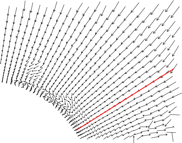
Figure 2: A time snapshot of the $\phi$ averaged poloidal magnetic field direction. The arrows indicate direction not magnitude. The region is the same as that which is plotted in figure 1. The red line indicates the approximate boundary of the funnel. The arrows end approximately on a circle that is the inner calculational boundary. The plot is provided courtesy of John Hawley.

5.4 Non Radial Field Geometry

We verify the near radial field geometry in the funnel in figure 2 which is a plot of the poloidal field direction averaged over $\phi$ in a constant time snapshot. The poloidal field is radial on the boundary surfaces 2 and 4 of the Gaussian pillbox of figure 1. This does not support the notion of $S^{\perp}$ flowing along the field lines from the funnel wall, as discussed in section 3.3, then following abrupt bends of the field lines toward the radial direction, so as to mimic a source of radial Poynting flux at $1.2M<r<1.4M$. Near the horizon, at lower latitudes in the funnel, $50^{\circ}<\theta<55^{\circ}$, where the strongest $S^{P}$ source is located (the red area in figure 1), the field is almost exactly radial all the way to the inner boundary. A small deviation from a radial poloidal field near the horizon would not be able to produce strong source of $S^{P}$ in Poynting’s theorem. Furthermore, if the poloidal field randomly oscillates about the radial direction (due to turbulence or numerical artifacts), near the horizon, then the oscillations in the Poynting flux would average to zero in the time averaged plot in figure 1. At higher latitudes in the funnel, $30^{\circ}<\theta<50^{\circ}$, there is a region of rapid poloidal field variation right near the inner boundary. The fluid is clearly highly turbulent, possibly a sign of reflections from the inner computational boundary. If the strong turbulence is physical, combined with the $U_{A}>>1$ condition, this would provide strong magnetic pressure gradients that prevent the tenuous plasma from flowing force-free into the horizon. This is the condition described in section 5.3.2 that is most conducive to a GHM dynamo.

6 Conclusion

In this paper, we studied simulations of a magnetically dominated funnel of a rapidly rotating black hole, $a/M=0.998$. A source region that is responsible for creating over 72% of $S^{P}$ transported through funnel during the interval $2000M<t<8080M$ of the simulation was identified. Similarly, one can conclude that $<28\%$ of $S^{P}$ emerging from the ergospheric funnel is from an inner boundary source, near the horizon. The small residual $S^{P}$ injected from the boundary into the accretion wind can be considered of electrodynamic origin. The distribution of $S^{P}$ in figure 1 is in contrast to the Blandford-Znajek solution in which essentially all the $S^{P}$ is of electrodynamic origin, i.e., it emanates from the horizon and passes through the accretion wind with minimal interaction, thereby maintaining a virtually constant value along each poloidal flux tube throughout the ergosphere. The existence of the electromagnetic source within the simulation was corroborated by existence of a cospatial electromagnetic angular momentum source using an entirely different data reduction method. Both of these results follow directly from the numerical data in Krolik et al (2005).

There were two possible physical sources for $S^{P}$ in the funnel, there is the $\mathbf{J}\cdot\mathbf{E}$ source (associated with GHM inertial currents) and $S^{\perp}$. By time averaging Faraday’s law it was shown that $\mid<F_{\phi\theta}>\mid\gg M\mid<F_{\phi t}>\mid$. The only source for both $S^{P}$ and $<T_{\phi}^{\;r}>$ in Poynting’s theorem that is consistent with Faraday,s law was shown to be $\mathbf{J}\cdot\mathbf{E}=F_{t\theta}J^{\theta}$. It was also pointed out that the decay of stored field energy, $d\epsilon/dt$ could be the primary source of $S^{P}$. This would suggest that the simulation is spontaneously creating energy and might be fatally flawed. In general, there could be a mix of numerical artifacts, $S^{\perp}$ and $\mathbf{J}\cdot\mathbf{E}$ that contribute to Poynting’s theorem. This can not be sorted out without further numerical work.

The analysis presented above suggests some interesting physical possibilities and highlights the need for further analysis of 3-D simulations about rapidly rotating black holes ($a/M=0.998$) in order to clarify the physics that creates $S^{P}$. Ideally, the 3-D simulation should be redone in ingoing Kerr-Schild coordinates (to eliminate boundary reflections a the horizon) and preferably a conservative code. At present, there is no code efficient enough to handle the large computing times required. Whether this approach or the De Villiers and Hawley (2003) approach is used, at least three consecutive time snapshots are needed in order to find the current distribution from Ampere’s Law at each coarse time step data dump. It is likely that $J^{\perp}$ is highly turbulent near the event horizon, so it would be important to then time average the current distribution. Higher resolution (particularly in the $\theta$ direction) might be required to resolve the issue of whether the source in figure 1 is from $J^{\perp}E_{\perp}$, $S^{\perp}$ or $d\epsilon/dt$. It would be prudent, if further calculations in Boyer-Lindquist coordinates are pursued, to locate the inner calculational boundary inside of the fast magneto-sonic surface at $r\approx 1.065M$ (inner order to overcome potential reflections). Such future detailed analysis would determine if there is some new interesting physics or just some unforseen numerical errors in KDE.

On a more general note, even though the simulations of De Villiers et al (2003); Hirose et al (2004); De Villiers et al (2005a, b); Krolik et al (2005); McKinney and Gammie (2004); McKinney (2005) are very impressive mathematically for their ability to self consistently solve a very complicated problem, one must ask if they are representative of the astrophysical world. It was discussed in McKinney (2005) that a radial field builds up in the funnel for any seed field configuration in the torus except for a purely toroidal field. This implies something generic about the result. The radial field always grows to seek a pressure balance with the inflow at the inner edge of the disk, therefore the mass accretion rate sets the field strength and the power output of the funnel. If this is a generic property of accretion disks then why are the vast majority ($\sim 90\%$) of quasars radio quiet. This tight coupling of the accretion rate to jet power seems to be a serious drawback of the results. From an astrophysical perspective, it would seem preferable to develop simulations of scenarios like those described in Spruit and Uzdensky (2005) in order to describe the full panoply of quasar radio emissivity properties.

References

- Blandford and Znajek (1977) Blandford, R. and Znajek, R. 1977, MNRAS. 179, 433
- Camenzind and Khanna (2000) Camenzind, M. and Khanna, R. 1999, Nuovo Cimento B115, 815
- Campanelli et al (2001) Campanelli, M., Khanna, G., Laguna, P., Pullin, J., Ryan, M. 2001, Class.Quant.Grav. 18, 1543
- De Villiers (2005) De Villiers, J.2005 in preparation (private communication).
- De Villiers and Hawley (2003) De Villiers, J., Hawley, 2003, ApJ 589 458
- De Villiers et al (2003) De Villiers, J., Hawley, J., Krolik, 2003, ApJ 599 1238
- De Villiers et al (2005a) De Villiers, J., Hawley, J., Krolik, K.,Hirose, S. 2005, astro-ph/0407092
- De Villiers et al (2005b) De Villiers, J., Hawley, J., Krolik, K.,Hirose, S. 2005, ApJ 620878
- Gammie et al (2003) Gammie, F., McKinney J.,T th, G. ApJ 589 444
- Hirose et al (2004) Hirose, S., Krolik, K., De Villiers, J., Hawley, J. 2004, ApJ 606, 1083
- Koide (2003) Koide, S. 2003 Phys Rev D67104010
- Koide et al (2002) Koide, S., Shibata, K., Kudoh, T. and Meier, D. 2002, Science 295, 1688
- Komissarov (2004) Komissarov, S. 2004, MNRAS 350, 407
- Komissarov (2005) Komissarov, S. 2005, MNRAS 359, 801
- Krolik et al (2005) Krolik, K., Hawley, J., Hirose, S. 2005, ApJ 622, 1008
- McKinney and Gammie (2004) McKinney, J. and Gammie, C. 2004, ApJ 611977
- McKinney (2005) McKinney, J. 2004, ApJL 6305
- Penrose (1969) Penrose, R. 1969, Nuovo Cimento 1, 252
- Phinney (1983) Phinney, E.S. 1983, PhD Dissertation University of Cambridge.
- Punsly (1991) Punsly, B. 1991, ApJ 372 424
- Punsly (2001) Punsly, B. 2001, Black Hole Gravitohydromagnetics (Springer-Verlag, New York)
- Punsly and Coroniti (1990) Punsly, B. and Coroniti, F. 1990, ApJ 354 583
- Semenov et al (2004) Semenov, V., Dyadechkin, S. and Punsly, B. 2004, Science 305978
- Spruit and Uzdensky (2005) Spruit, H. and Uzdensky, D., ApJ 629 965
- Thorne et al (1986) Thorne, K., Price, R. and Macdonald, D. 1986, Black Holes: The Membrane Paradigm (Yale University Press, New Haven)