Long-term flaring activity of XRF 011030 observed with BeppoSAX

We present the spectral and temporal analysis of the X-ray flash XRF 011030 observed with BeppoSAX. This event is characterized by a very long X–ray bursting activity that lasts about 1500 s, one of the longest ever observed by BeppoSAX. In particular, a precursor and a late flare are present in the light curve.

We connect the late X–ray flare observed at about 1300 s to the afterglow emission observed by Chandra and associate it with the onset of the afterglow emission in the framework of external shock by a long duration engine activity. We find that the late X-ray flare and the broadband afterglow data, including optical and radio measurements, are consistent either with a fireball expanding in a wind environment or with a jetted fireball in an ISM.

1 Introduction

Prompt and afterglow emission in GRB show different temporal and spectral properties and are usually attributed to different mechanisms, more specifically, internal and external shocks, respectively. During the prompt emission, the spectrum is hard and shows strong spectral evolution from hard to soft. However, the afterglow emission is much softer, and its spectral index remains roughly constant during the whole emission from early to late observations (Frontera et al. 2000; Piro et al. 2002). The transition from one regime to the other takes place from a few tens to a few thousand seconds after the burst. In this phase, a variety of temporal behaviour is observed in different bursts, likely due to the contribution of both prompt and afterglow emission. Most intriguing is the presence of X-ray flares, such as that observed in XRF 011030 .

Indeed, several bursts observed by BeppoSAX showed the presence of X–ray flares from tens of seconds (e.g., GRB 970228 (Frontera et al. 1998) and GRB 980613 (Soffitta et al. 2002)) to several minutes (e.g., GRB 011121 and X-Ray Rich XRR 011211 (Piro et al. 2005)) after the burst. These flares have a soft spectrum consistent with that of the late afterglow. Furthermore, they connect with the late afterglow emission with a power law $F\propto(t-t_{0})^{-\alpha}$. For early ($<$ 1 minute) X–ray flares, the origin of the time $t_{0}$ is consistent with the onset of the prompt emission. For later ($\gtrsim$ 100 s) X–ray flares, $t_{0}$ needs to be shifted to the onset of the flare (Piro et al. 2005).

More recently, X–ray flares taking place in a similar time period have been observed by Swift (Gehrels et al. 2004) in a larger number of bursts, about one half of the sample (O’Brien et al. 2006) . Swift observations are providing a big advance in the understanding of this phenomenon and its possible relationship with the central engine. In particular, the discovery in GRB 050502B (Burrows et al. 2005a) of a giant flare, $\sim$ 700 s after the trigger, with an energy comparable to that of the burst itself, suggests that the central engine is undergoing long periods of strong activity.

Swift observations confirm that X-ray flares have a spectrum that is globally softer than the prompt emission, i.e., the peak energy $E_{peak}$ is of the order of a few keV (Falcone et al. 2006). In some cases (GRB 050126, GRB 050219a, and GRB 050904), no significant evidence of spectral evolution is detected, and the spectrum of the flare is consistent with that observed in the late afterglow (Tagliaferri et al. 2005; Goad et al. 2006; Burrows et al. 2005b). The light curve connecting the flare with the late afterglow can be reasonably well-fitted by the $(t-t_{0})^{-\alpha}$ power law (Tagliaferri et al. 2005). However, in other cases (XRF 050406 (Romano et al. 2006), GRB 050502B (Burrows et al. 2005a; Falcone et al. 2006), GRB 050421, GRB 050607, GRB 050730, and GRB 050724 (Burrows et al. 2005b)), hard-to-soft spectral evolution was observed during the flare.

Several scenarios were proposed to explain the X-ray flare phenomenon (Zhang et al. 2006). Burrows et al. (2005a) propose that the central engine releases energy for a long time, and internal shocks then produce a long duration prompt emission. In the framework of the forward-reverse shock scenario, Fan & Wei (2005) have shown that, adopting different values for the forward and the reverse shock parameters, the reverse shock synchrotron radiation can dominate in the X–ray band producing a flare. In another scenario, late X–ray flares mark the beginning of the afterglow emission, and they are produced by a thick shell fireball (long duration engine activity) through an external shock (Piro et al. 2005). Very recently, Wu et al. (2005) have shown that X–ray flares can be produced in the context of both late internal and late external shocks. They assume that the central engine releases energy in two episodes (i.e., an early and a late shell are ejected). They applied their model to four Swift GRB and found that XRF 050406 and GRB 050607 flares can be explained both with late internal or external shocks.

In this paper, we present a complete analysis of XRF 011030 observed with BeppoSAX. It shows outburst activities, with the last detected flare occurring about 1300 s after the burst. We investigate the origin of this late X–ray flare. As mentioned above, several models could explain this phenomenon. Here we have carried out a detailed analysis of the model in which the flare is produced by the interaction of the fireball with the external medium. We check if the model can consistently account for the broadband data – from radio to X-rays. We then derive the main parameters of the fireball, including the density profile of the surrounding medium. We have also tested this model for the X–ray flare occurring in GRB 011121.

We describe the observations of XRF 011030 in Sect. 2 and perform its temporal and spectral analysis in Sect. 2.1 and 2.2, respectively. In Sect. 3 we discuss late flares in the context of different variants of the external shock model. In Sect. 4 we apply a long duration engine activity (thick shell) model to the late flare appearing in XRF 011030 and in GRB 011121 , and we explain it as the onset of the afterglow emission. In particular, in Sect. 4.1, we study the XRF 011030 late afterglow emission taking into account the presence of a break occurring between $10^{4}$ and $10^{6}$ s after the burst. In Sect. 5 we use information on XRF 011030 from the optical and the radio band to further constrain the model. Our results and conclusions are summarized in Sect. 6.

2 Observations and data reduction

The X-ray flash XRF 011030 was detected by the BeppoSAX Wide Field Camera (WFC) no. 1 on October 30th, 2001, at 06:28:02, without any counterpart in the Gamma Ray-Burst Monitor (GRBM) (Gandolfi 2001).

The peak flux is $7.5\times 10^{-9}$erg s^-1cm^-2, and the total fluence of the source between 2 and 26 keV is equal to $1.2\times 10^{-6}$ erg cm^-2, consistent with the typical value observed in the same range for normal GRB (Amati et al. 2002).

The X-ray afterglow of XRF 011030 was identified by Chandra in a 47 ks exposure beginning on November 2001, at 9.73 UT and in a second one of 20 ks performed on November 2001, at 29.44 UT (Harrison et al. 2001). The localization of the X–ray afterglow was consistent with the position of a radio transient (Taylor et al. 2001). The radio source was detected on November 2001, at 8.80 UT near the centre of the WFC error circle at (epoch 2000) R.A.=20:43:32.3, Dec.=+77:17:18.9 with an error of $\pm 1\arcsec$. In this paper, we have used the results of the analysis of the Chandra data performed by D’Alessio et al. (2005). The spectrum between 2 and 10 keV is fitted by a power law with a photon index $\Gamma=1.72^{+0.19}_{-0.20}$ (Table 1). Several optical observations were carried out, but none of them succeeded in associating an optical counterpart with XRF 011030. The tighest upper limits are R$>$21 at 0.3 days after the burst (Vijay et al. 2001) and R$>$23.6 at 2.7 days after the burst (Rhoads et al. 2001).

The precise Chandra localization allowed the association of the burst with a faint irregular blue galaxy observed by the Hubble Space Telescope and the Keck. The photometric observations of this galaxy suggest a redshift smaller than $z\sim$3.5, while the low brightness of the galaxy suggests that $z>$ 0.6 (Bloom et al. 2003). Since the observations allow us to establish only a wide range of redshift values, in our analysis we assume $z$=1.

2.1 Temporal analysis of XRF 011030

We produced background subtracted light curves of XRF 011030 normalized to the detector effective area exposed to the source. The source remained in the field of view (f.o.v.) of the WFC for about 1 day. A significant source flux above the background level is detected until $\sim$ 1600 s (see Fig. 1). A main pulse, lasting $\sim$ 400 s, starts $\sim$ 300 s after a fainter preceding event. The main event is also followed by an X–ray flaring activity, 200 s long, which appears $\sim$ 1300 s after the first pulse. This X–ray flare has duration and flux similar to the pulse preceding the main event.

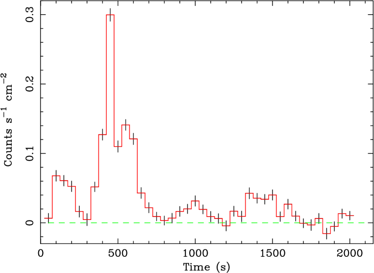
Figure 1: Light curve of XRF 011030 in the BeppoSAX WFC (2-26 KeV) with a temporal resolution of 50 s. The main pulse (300-700 s) is preceded by a fainter event (0-300 s) and is followed by a late X–ray flare (1300-1550 s).

As the event is an X–ray flash, its spectrum is soft by definition. Thus, we cannot expect to find such substantial spectral differences as those find in GRBs between the phases of precursor, prompt emission, and late X–ray flare, i.e., with a precursor and late flare markedly softer than the prompt emission (Piro et al. 2005). In any case, due to the similarities of the bursting activities that preceded and followed the main pulse in XRF 011030 to those observed in GRB 011121 (Piro et al. 2005), in the following we refer to these two pulses as precursor and flare, respectively.

After about 1600 s, no signal is detected and we can only estimate upper limits on the flux. The light curve of XRF 011030 with the upper limits between 1600 s and $10^{5}$ s together with the late afterglow emission detected by Chandra is shown in Fig. 2.

Figure 2: XRF 011030 light curve with the BeppoSAX upper limits on the flux fixed at 3$\sigma$ above the background fluctuations. The late afterglow emission detected by Chandra is shown in red squares. [See the electronic edition for a colour version of this figure.]

2.2 Spectral analysis

We extracted the spectrum between 2–26 keV from the WFC data. In the spectral fitting, we tested a simple power law model (with and without photoelectric absorption), a broken power law model, and a black-body model. The results of our spectral analysis are summarized in Table 1. All errors are quoted at 1 $\sigma$ (68% confidence level).

The whole spectrum of XRF 011030, integrated from 0 s to 1550 s can be described by a simple power law (Fig. 3) with a photon index $\Gamma$=$1.84^{+0.17}_{-0.16}$, consistent with the simple power law photon index $\Gamma=1.9\pm 0.1$ determined by Heise (2003). The fit with this model gives $\chi^{2}_{\nu}=0.83$; 25 degrees of freedom (d.o.f.).

Figure 3: $\nu$F_ν spectrum of the total event. The solid line represents the fit of XRF 011030 with a simple power law model.

A fit of the spectrum with a broken power law having the photon index $\Gamma_{1}$ free to vary and the photon index $\Gamma_{2}$ fixed to the typical value 2.5 (Amati et al. 2002) did not bring a significant improvement of $\chi^{2}$. Also, the fit with a power law with a photoelectric absorption did not bring a significant improvement of $\chi^{2}$, and led to an upper limit on the absorption column density $N_{H}<1.5\times 10^{23}cm^{-2}$ at z=1. Finally, the fit with a black-body model gives a $\chi^{2}_{\nu}$ value greater than 2, and it can thus be rejected.

We studied the spectral evolution of XRF 011030 by dividing the data into four intervals: the precursor (from 35 s to 280 s), the first segment of the prompt emission (from 280 s to 500 s), the second segment of the prompt emission (from 500 s to 1200 s), and the flare (from 1300 s to 1550 s). We observed only a marginal spectral variability.

The precursor spectrum is well-described by a simple power law with a photon index $\Gamma$=$2.61^{+0.76}_{-0.61}$, marginally steeper than the spectrum of the main event. This fit gives $\chi^{2}_{\nu}$=0.81; 25 d.o.f. The precursor can be also described by a black-body model with a temperature $kT$=$0.90^{+0.19}_{-0.15}\leavevmode\nobreak\ keV$ (see Fig. 4) and $\chi^{2}_{\nu}$=0.96; 25 d.o.f. This result is interesting because there is only one burst, observed by GINGA, whose spectrum is consistent with a black body (Murakami et al. 1991). However, we cannot discriminate between these two models.

Figure 4: $\nu$F_ν spectrum of the precursor. The solid line is the fit of the precursor with a black-body model.

The first and the second parts of the prompt emission are both fitted by a simple power law; for the first part, the photon index is $\Gamma$=$1.78^{+0.17}_{-0.16}$ and $\chi^{2}_{\nu}$=1.24; 25 d.o.f., and for the second one, $\Gamma$=$1.63^{+0.33}_{-0.30}$ and $\chi^{2}_{\nu}$=1.48; 25 d.o.f.

Finally, the late X–ray flare is also fitted by a simple power law. Its spectrum is marginally steeper than those of the main event, as we also found in the case of the precursor: $\Gamma$=$2.10^{+0.83}_{-0.64}$ with $\chi^{2}_{\nu}$=1.51; 25 d.o.f.

Table 1: Results of the spectral analysis of XRF 011030. The models used are: Power Law (PL), BroKeN power law (BKN), Power Law plus photoelectric ABSorption (PL+ABS) and Black Body (BB).

name	interval	model	photon	$N_{H}$	$E_{b}$	kT	$Flux_{2-26\leavevmode\nobreak\ keV}$	$\chi^{2}_{\nu}$	$\nu$
	(s)		index $\Gamma$	($cm^{-2}$, z=1)	(keV)	(keV)	[$erg\cdot cm^{-2}\cdot s^{-1}$]
total	0-1550	PL	$1.84^{+0.17}_{-0.16}$	—	—	—	$1.3\cdot 10^{-9}$	0.83	25
event	—	BKN	$1.77^{+0.19}_{-0.23}$	—	$<11$	—	$1.3\cdot 10^{-9}$	0.81	24
	—	PL+ABS	$1.88^{+0.27}_{-0.14}$	$<1.5\cdot 10^{23}$	—	—	$1.2\cdot 10^{-9}$	0.86	24
precursor	35-280	PL	$2.61^{+0.76}_{-0.61}$	—	—	—	$5.8\cdot 10^{-10}$	0.81	25
	—	PL+ABS	$2.44^{+2.06}_{-0.44}$	$<7\cdot 10^{22}$	—	—	$5.5\cdot 10^{-10}$	0.87	24
	—	BB	—	—	—	$0.90^{+0.19}_{-0.15}$	$3.7\cdot 10^{-10}$	0.96	25
burst	280-500	PL	$1.78^{+0.17}_{-0.16}$	—	—	—	$2.5\cdot 10^{-9}$	1.24	25
part 1	—	BKN	$1.59^{+0.23}_{-0.27}$	—	$9.1^{+4.0}_{-2.1}$	—	$2.3\cdot 10^{-9}$	1.08	24
	—	PL+ABS	$2.23^{+0.36}_{-0.31}$	$<4.4\cdot 10^{23}$	—	—	$2.1\cdot 10^{-9}$	1.16	24
burst	500-1200	PL	$1.63^{+0.33}_{-0.30}$	—	—	—	$8.9\cdot 10^{-10}$	1.48	25
part 2	—	BKN	$0.39^{+1.49}_{-0.31}$	—	$<4.4$	—	$7.8\cdot 10^{-10}$	1.6	24
	—	PL+ABS	$1.93^{+0.74}_{-0.53}$	$<8.6\cdot 10^{22}$	—	—	$8.1\cdot 10^{-10}$	1.65	24
X-ray late	1300-1550	PL	$2.10^{+0.83}_{-0.64}$	—	—	—	$4.9\cdot 10^{-10}$	1.51	25
flare	—	BKN	$4.18\pm 10$	—	$<3.0$	—	$5.8\cdot 10^{-10}$	1.7	24
	—	PL+ABS	$2.10^{+3.93}_{-0.64}$	$<1.3\cdot 10^{23}$	—	—	$4.9\cdot 10^{-10}$	1.72	24
afterglow1	$(9.24-9.71)\cdot 10^{5}$	PL+ABS	$1.72\pm 0.20$	$2.96^{+0.60}_{-0.65}\cdot 10^{21}$	—	—	$5.8\cdot 10^{-14}$	0.76	9

¹From D’Alessio et al. (2005); the flux is in the 2-10 keV range.

3 The late X–ray flare in the context of external shock models

Among the different models proposed for X-ray flares (Zhang et al. 2006), we choose to analyse in detail some of the models based upon an external shock origin, motivated by the spectral similarity observed in the flare and afterglow phases, straightforwardly accounted for in this scenario. A detailed analysis is carried out to check the capability of the model to account for the whole set of broadband data.

In what follows, we first try to explain the late flare of XRF 011030 as being due to external shock in a ”standard” fireball model (i.e., thin shell case, Sari & Piran (1999)), with a continuous or discontinuous density profile. Since the flare cannot be described by this model, considering the similarity of XRF 011030 with GRB 011121, we finally explain it by shifting the origin of time $t_{0}$ to the instant of the flare, which corresponds to a thick shell fireball.

3.1 The Fireball Model: the standard “thin” shell case

In a “standard” approach, the Fireball Model assumes a thin shell (Sari & Piran 1999) that expands with spherical symmetry either in a constant density medium or in a wind profile environment. In this framework, the emitted flux reaches its maximum at the deceleration radius $r_{0}$ and then starts to decrease. However, it does this too slowly to be consistent with the onset and decay of the flare. This appears clearly in Fig. 5, where the calculated light curve for a thin shell fireball expanding in an ISM is shown.

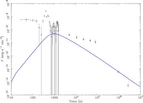
Figure 5: X–ray light curve of XRF 011030 for a standard thin shell fireball expanding in an ISM with $E_{53}=0.03$, $\Gamma_{0}=45$, $n=1$, $\varepsilon_{e}=0.3$, $\varepsilon_{B}=0.05$, and $p=2.1$.

Moreover, we note that a thin shell fireball also fails to explain the emission at about 1000 s. In such a case, the deceleration time of the fireball $t_{dec}$ is greater than the duration of the central engine activity $t_{eng}$, thus prompt and afterglow emission are well separated, and one would expect no emission between these two phases.

3.2 Model with a discontinuous density profile

A discontinuous density profile can be produced by a variable activity of wind emission or by interaction of the wind bubble with the external uniform medium. When the fireball expands in a medium characterized by a sudden increase of density, one could expect that a larger number of photons is produced and the flux increases quickly. This is true only when the electron cooling frequency $\nu_{c}$ is greater then the observational frequency $\nu_{obs}$. On the contrary, when $\nu_{c}<\nu_{obs}$, the emitted flux is independent of the density profile both during the slow cooling and the fast cooling regimes (Panaitescu & Kumar 2000). Let us then verify if the cooling frequency could be located above the X-ray range at the time of the flare.

A fireball expanding in an ISM decelerates at a time $t_{dec}$ (Panaitescu & Kumar 2000):

$$t_{dec}\simeq 46.7E_{51}^{1/3}n^{-1/3}\Gamma_{0,2}^{-8/3}\leavevmode\nobreak\ s.$$ (1)

During the deceleration phase (for $t>t_{dec}$), the cooling frequency $\nu_{c}$ is given by (Panaitescu & Kumar 2000):

$$\nu_{c}\simeq 3.4\times 10^{16}E_{51}^{-1/2}n^{-1}\varepsilon_{B,-2}^{-3/2}t_{3}^{-1/2}\leavevmode\nobreak\ Hz.$$ (2)

Except for very low values of the Lorentz factor, $\Gamma_{0}<30$, the flare occurs during the deceleration phase and the cooling frequency $\nu_{c}$ is given by Eq. 2. This equation indicates that, for typical XRF energies and parameter values, at the time of the flare, $t_{3}\simeq 1$, the cooling frequency $\nu_{c}$ could be higher than the observational frequency $\nu_{obs}$ (that is, in the X–ray band) only for small values of density, $n<0.07$. During the deceleration phase, $\nu_{c}$ decreases with time and will pass below the X-ray range at later times.

If the fireball starts its expansion in a wind density profile, the deceleration time $t_{dec}$ is (Panaitescu & Kumar 2000):

$$t_{dec}\simeq 6.67E_{51}A_{*,-2}^{-1}\Gamma_{0,2}^{-4}\leavevmode\nobreak\ s$$ (3)

and during the deceleration regime

$$\nu_{c}\simeq 3.77\times 10^{16}E_{51}^{1/2}A_{*,-2}^{-2}\varepsilon_{B,-2}^{-3/2}t_{3}^{1/2}\leavevmode\nobreak\ Hz.$$ (4)

Also in this case, for $A_{*}\lesssim 10^{-3}$, $\nu_{c}$ can be higher than $\nu_{obs}$ at the flare time. Moreover, now $\nu_{c}$ increases with time, and therefore the X-ray afterglow emission will remain sensitive to density variations. Thus, for a suitable range of parameters, at the time of the flare the X-ray emission can be sensitive to density. However, the duration and amplitude of the flare are not consistent with the kinematic upper limit recently established by Ioka et al. (2005) on the flares produced by the interaction of the fireball with density discontinuities. In particular, if we assume to observe GRB on axis, this upper limit is (Ioka et al. 2005):

$$\frac{\Delta F_{\nu}}{F_{\nu}}\leq\frac{4}{5}f_{c}^{-1}\frac{F}{\nu F_{\nu}}\frac{\Delta t}{t-t_{0}},$$ (5)

where $f_{c}^{-1}\sim(\nu_{i}/\nu_{c})^{(p-2)/2}$ is the fraction of cooling energy and $F/\nu F_{\nu}\sim(\nu_{obs}/\nu_{c})^{(p-2)/2}$ for $\nu_{c}<\nu_{obs}$. The flare duration is $\Delta t\simeq 200$ s in XRF 011030, and the time of the flare occurrence is $(t-t_{0})\simeq 1300$ s, where the time is counted from $t_{0}$, i.e., in the case of a thin shell, from the initial trigger. Thus $\Delta t/t\sim$0.15, and with typical parameters values, Eq. 5 implies $\Delta F_{\nu}/F_{\nu}\leq$ 0.25, while from the X–ray data of XRF 011030 we derive $\Delta F_{\nu}/F_{\nu}\sim$ 3.6.

We point out that the case discussed above applies only to a density discontinuity with a shell geometry. Dermer & Mitman (1999) have shown that a clumpy medium would be able to produce high variable light curves through external shock if the clouds radius is very small in comparison to their distance from the central engine. This process can explain X-ray flares up to thousand of seconds (Dermer 2005).

3.3 Long duration engine activity: the thick shell model

In the following, we show how we can describe the flare in the context of the external shock scenario by shifting the origin of the time $t_{0}$ to the onset of the flare. From a theoretical point of view, the onset of the external shock depends on the dynamical regime of the fireball that is strictly related to the “thickness” of the shell (Sari & Piran 1999), i.e., to the duration of the engine activity. In fact, a shell is defined as being thin or thick depending on its thickness $\Delta=ct_{eng}$, where $t_{eng}$ is the duration of the engine activity, and also on its initial Lorentz factor $\Gamma_{0}$. The shell is defined to be thick if $(E/nm_{p}c^{2})^{1/3}\Gamma_{0}^{-8/3}<\Delta$ (Sari & Piran 1999). For our purpose, we rewrite the above equation substituting the deceleration time given in Eq. (3) of Piro et al. (2005), obtaining $t_{eng}\gtrsim t_{dec}$ for the thick shell condition. Most of the energy is transferred to the surrounding material at $t_{dec}$ for thin shells or at $t_{eng}$ for thick shells. In the latter case, the peak of the afterglow emission therefore coincides with $t_{eng}$. Also, the afterglow decay will be described by a power-law only if the time is measured starting from the time at which the inner engine turns off, i.e., $t_{0}\simeq t_{eng}$. According to Lazzati & Begelman (2006), this should happen when the central engine releases most of the energy during the last phase of its activity. In this context, the flare would thus be produced by the external shock caused by an energy injection lasting until the time of the flare occurrence, i.e., $t_{eng}\approx 1300$s. The hypothesis of external shock for the flare offers a straightforward explanation of the spectral similarity with the late afterglow data. We also notice that in this model the early afterglow emission is mixed with the (internal shock) GRB emission (Sari & Piran 1999). In this context, the emission observed at 1000 s can be attributed to internal shock while the flare represents the onset of the afterglow emission.

To develop our model, we used the prescriptions of the so-called standard fireball model (Panaitescu & Kumar 2000). They offer analytic solutions only at distances greater than the deceleration radius $r_{0}$. But we are also interested in the so-called coasting and transition phases (Zhang & Meszaros 2004) because we want to study and to reproduce the shape of the flare, its rise included. As mentioned above, we have taken into account the thick shell variant by introducing a time shift $t_{0}$, i.e., implying that most of the energy for the external shock is carried at $t_{0}\approx t_{eng}$. We thus numerically solved the basic equations of the fireball model. The program requires the parameters of the model, namely the initial value of the Lorentz factor of the relativistic shell $\Gamma_{0}$, the energy value in unity of $10^{53}$ erg $E_{53}$, the electron population index $p$, the fraction of energy going into relativistic electrons $\varepsilon_{e}$, the fraction of energy going in magnetic field $\varepsilon_{B}$, and the density of the external medium $n$ (cm^-3) or $A_{*}$ (cm^-1) as input. The density profile is described by the law $n=3.0\cdot 10^{35}A_{*}r^{-s}$, where in the case of an ISM, $s=0$, while in the case of a wind profile environment, $s=2$.

When not stated otherwise, we have taken $E_{53}$=0.03, assuming that all the kinetic energy is converted in $\gamma$-rays and that the redshift is $z=1$. From our spectral analysis, we find $p=2.1$. To determine the other parameters values, we performed a study devoted to understanding how they influence the calculated light curve.

We investigated the effect of model parameters on the X-ray light curve produced by a thick shell fireball with spherical symmetry expanding in an ISM. The origin of the time, $t_{0}$, is shifted to the instant of the flare, 1300 s. We show the X–ray flux between 2-10 keV obtained by numerical integration of the specific energy flux.

First we find, according to the fact that the X-ray emission is typically above the cooling frequency, particularly at late times, that the density $n$ and $\varepsilon_{B}$ only have a marginal effect on the normalization of the X-ray light curve. Figure 6 shows, for example, the effects of the density $n$ of the external medium in which the fireball expands. Differences are appreciable only at early times, when the observational frequency $\nu_{obs}$ is smaller than the cooling frequency $\nu_{c}$.

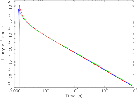
Figure 6: Effects of density $n$ of the external medium on the X–ray light curve with the origin of the time shifted to $t_{0}$=1300 s. For the red curve $n$=5 $cm^{-3}$, for the blue curve $n$=1 $cm^{-3}$, and for the green curve $n$=0.1 $cm^{-3}$. The X–ray light curve peak shows a small increase with $n$. The other model parameters are $E_{53}$=0.03, $\Gamma_{0}$=85, $\varepsilon_{e}$=0.01, $\varepsilon_{B}$=0.05, and $p$=2.2.

The effects of the parameters $E_{53}$ and $\varepsilon_{e}$ are presented in Fig. 7. The normalization of the X-ray light curve depends mostly on the product of $E_{53}$ and $\varepsilon_{e}$, and follows a roughly linear dependence (for $p\approx 2.2$).

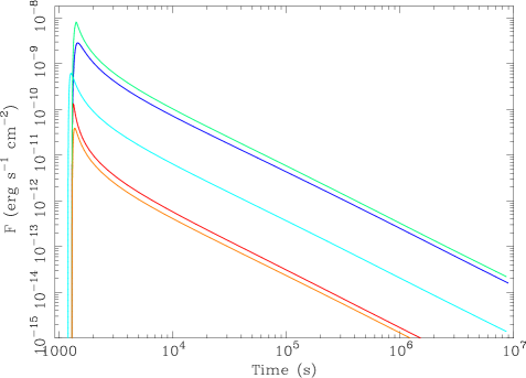
Figure 7: Effects of the energy $E_{53}$ and $\varepsilon_{e}$ on the X–ray light curve with the origin of the time shifted to $t_{0}$=1300 s. For the green curve $E_{53}=0.03$ and $\varepsilon_{e}=0.1$, for the blue curve $E_{53}=0.3$ and $\varepsilon_{e}=0.01$, for the light blue curve $E_{53}=0.03$ and $\varepsilon_{e}=0.01$, for the red curve $E_{53}=0.003$ and $\varepsilon_{e}=0.01$, and finally for the orange curve $E_{53}=0.03$ and $\varepsilon_{e}=0.001$. The other model parameters are $n$=1, $\Gamma_{0}$=85, $\varepsilon_{B}$=0.05, and $p$=2.2. Note, as the emitted flux increases with $E_{53}$ and $\varepsilon_{e}$, that these parameters have about the same amount of influence in determining the normalization factor of the X–ray light curve.

Figure 8 shows the effects of the initial Lorentz factor $\Gamma_{0}$. Its value influences both the height and the wideness of the peak in the X–ray light curve. The greater $\Gamma_{0}$ is, the higher and narrower the peak is. For $t\gg t_{0}$, i.e., when the deceleration phase has been reached for the different values of $\Gamma_{0}$, the light curve is independent of $\Gamma_{0}$.

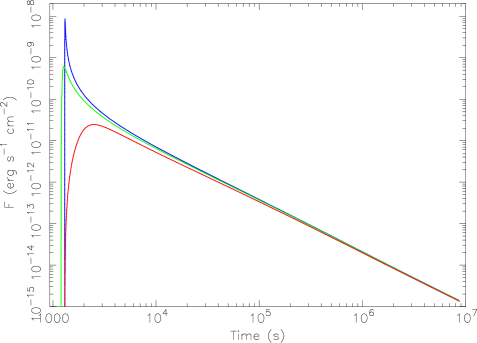
Figure 8: Effects of the initial Lorentz factor $\Gamma_{0}$ on the X–ray light curve with the origin of the time shifted to $t_{0}$=1300 s. The blue curve was obtained for $\Gamma_{0}=200$, the green curve for $\Gamma_{0}=85$, and the red curve for $\Gamma_{0}=30$. Note, as the peak in the curve increases with $\Gamma_{0}$, the other model parameters are $E_{53}$=0.03, $n$=1, $\varepsilon_{e}$=0.01, $\varepsilon_{B}$=0.05, and $p$=2.2.

4 External shock from long duration engine activity in XRF 011030 and GRB 011121

We applied the model described in the previous section to XRF 011030 and also to GRB 011121. In the case of XRF 011030, we studied the event both in an ISM and in a wind profile environment, producing the calculated light curves and finding a family of solutions corresponding to several choices of the model parameters. In Figs. 9 and 10 we report two possible solutions for a fireball expanding in an ISM and in a wind profile environment, respectively, with the origin of the time shifted to the onset of the flare, $t_{0}=1300$ s. Small changes ($\lesssim 10$%) of $t_{0}$ do not appreciably modify the results.

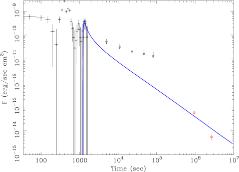
Figure 9: X–ray light curve of XRF 011030 in an ISM obtained shifting the origin of the time to the onset of the flare, $t_{0}=1300$s. The model parameters are $E_{53}=0.03$, $\Gamma_{0}=110$, $n=1$, $\varepsilon_{e}=0.2$, $\varepsilon_{B}=0.05$, and $p=2.1$.

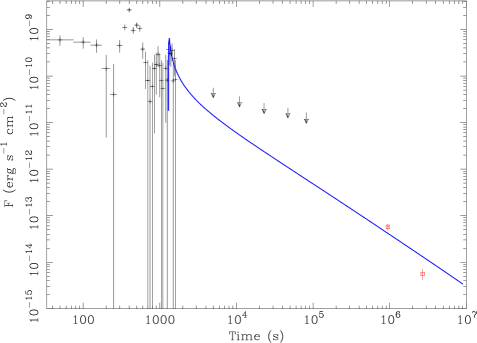
Figure 10: X–ray light curve of XRF 011030 in a wind obtained shifting the origin of the time to the onset of the flare, $t_{0}=1300s$. The model parameters are $E_{53}=0.03$, $\Gamma_{0}=50$, $A_{*}=0.05$, $\varepsilon_{e}=0.1$, $\varepsilon_{B}=0.05$, and $p=2.1$.

We find that the calculated light curves can describe the flare, both for a fireball expanding in a wind profile environment and for a fireball interacting with a uniform medium. These two light curves do not fit the late afterglow data; this will be discussed in the next section.

In the case of the flare of GRB 011121, we computed the light curve only for a fireball interacting with a wind density profile. In fact, Piro et al. (2005) established that the GRB 011121 X–ray and optical data are consistent with a fireball expanding in a wind environment due to the temporal decay observed in these two bands. Using their parameters and shifting $t_{0}$ to the onset of the flare, we find the light curve of Fig. 11. The model describes the flare and the late afterglow, in agreement with the analysis made by Piro et al. (2005).

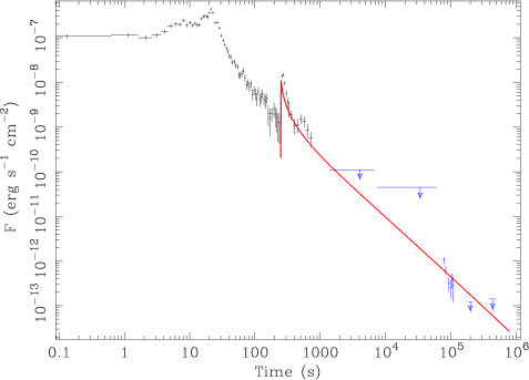
Figure 11: X–ray light curve of GRB 011121 for a fireball expanding in a wind with the origin of the time shifted to the instant of the flare, $t_{0}=250$ s. The model parameters are $E_{53}=0.28$, $\Gamma_{0}=130$, $A_{*}=0.003$, $\varepsilon_{e}=0.01$, $\varepsilon_{B}=0.5$, and $p=2.5$.

4.1 The interpretation of the break in the light curve of XRF 011030

In Fig. 2, we note that the backward extrapolation of the late afterglow flux detected by Chandra is not compatible with the upper limits observed by BeppoSAX, suggesting the presence of a temporal break.

First we considered the possibility that the temporal break is related to a spectral break, i.e., to the passage of the cooling frequency $\nu_{c}$ in the X-ray band. We first studied the case of a wind density profile, when $\nu_{c}$ increases with the time as $t^{1/2}$. Initially, $\nu_{c}$ can be smaller than $\nu_{obs}$, but there will be an instant at which it becomes greater than $\nu_{obs}$. This marks a break in the light curve, which becomes steeper by $\delta\alpha=0.25$.

The observational data of XRF 011030 suggest that the break occurs between $10^{4}$ and $10^{6}$ s after the burst. We thus require that $\nu_{c}$ passes in the X–ray band during this temporal range. Eq. (4) for a given time of the break $T_{b}$ links $A_{*}$ with $\varepsilon_{B}$. We derive $\varepsilon_{e}$ and $\Gamma_{0}$ values to reproduce the light curve of the flare as described in the previous section. $A_{*}$ is constrained from late X-ray data and also optical and radio data (see next section). Finally, the corresponding value of $\varepsilon_{B}$ is constrained from Eq. (4). We first attempt to find a broadband solution with the isotropic energy fixed to $E_{53}=0.03$ (see Sect. 3.3). In this case, we have problems fitting the radio data. We find a set of model parameters able to describe the emission observed in the X–ray and optical bands, but the corresponding radio light curve is always below the observational data. When the fireball expands in a stellar wind, the flux in the radio band goes as:

$$F_{\nu}\propto E_{53}^{1/3}A_{*}\varepsilon_{e,-1}^{-2/3}\varepsilon_{B,-3}^{1/3}.$$ (6)

The parameters $\varepsilon_{e}$ and $\varepsilon_{B}$ are determined by X-ray and optical data (see the next Sect. for more detail). Then, if we keep $E_{53}=0.03$ to obtain the right normalization of the radio light curve, we need to increase the wind density. On the other hand, this will also cause the normalization of the X–ray and optical light curves to increase and surpass the observational data. This has motivated us to assume an efficiency $\eta=0.1$ to convert the kinetic energy released by the central engine in $\gamma$–rays. This choice is supported by several authors. Guetta, Spada & Waxman (2001) and Kobayashi & Sari (2001) have argued that internal shocks convert the energy with an efficiency $\eta\sim 0.1-0.5$, and this was also recently supported by Swift observations (Zhang et al. 2006; Granot, Konigl & Piran 2006). Under this assumption (i.e., $E_{53}=0.3$) we find that it is possible to explain the radio data jointly with the X-ray and optical data, obtaining a broadband solution. In Fig. 12, we show the calculated X–ray light curve.

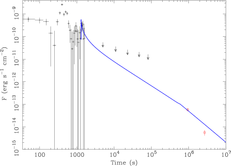
Figure 12: X–ray light curve of XRF 011030 in a wind with the origin of the time shifted to $t_{0}=1300s$. This solution also takes into account the radio and optical data. The model parameters are $E_{53}=0.3$, $\Gamma_{0}=60$, $A_{*}=0.055$, $\varepsilon_{e}=0.02$, $\varepsilon_{B}=0.001$, and $p=2.1$. We have assumed the efficiency in the conversion of the kinetic energy to be $\eta$=0.1.

It is interesting to note that before the break ($\nu_{c}<\nu_{obs}$), i.e., during the flare, the expected photon index is $\Gamma=(p/2+1)=2.05$, consistent with the value found in our spectral analysis (Sect. 1). After the break ($\nu_{c}>\nu_{obs}$), the expected photon index is $\Gamma=[(p-1)/2+1]=1.55$, which agrees with the value $\Gamma=1.72\pm 0.20$ found by D’Alessio et al. (2005) in the analysis of the Chandra data.

With regard to the fireball temporal evolution after the break, $\nu_{c}>\nu_{obs}$ (Panaitescu & Kumar 2002):

$$F\propto t^{-(3p-1)/4},$$ (7)

and we expect that the temporal decay index is $\alpha_{2}=1.325$. The analysis of Chandra data shows that after the break $\alpha_{2}=2.25\pm 0.60$ (D’Alessio et al. 2005), these values are marginally consistent.

Similar considerations can be made for a fireball expanding in an ISM. In this case, the cooling frequency $\nu_{c}$ decreases with the time as $t^{-1/2}$. Supposing $\nu_{c}>\nu_{obs}$ before the flare, there will be an instant when $\nu_{c}$ becomes smaller than $\nu_{obs}$ and a break occurs.

Now, after the break, the temporal decay is slower than the case of a wind density profile (Panaitescu & Kumar 2002):

$$F\propto t^{-(3p-2)/4}$$ (8)

and the temporal decay index expected after the break is $\alpha_{2}=1.075$, not consistent with the Chandra data. Moreover the spectrum after the break steepens, in disagreement with the spectral data.

In the ISM case, it is therefore even more difficult than in the wind case to explain the late afterglow emission without introducing a jet structure. The emission coming from a relativistic shell with jet symmetry is similar to the one of a spherical fireball, as long as the observer is on the jet axis, and the jet Lorentz factor $\gamma$ is greater than the inverse of its angular spread $\theta_{0}$ (Rhoads 1997). During its expansion, the fireball collects a growing amount of matter; thus, the Lorentz factor $\gamma$ decreases and there is an instant when $\gamma<\theta_{0}^{-1}$. At this time, the sideways spread of the jet becomes important and the observed area grows more quickly. This leads the flux to decrease more rapidly whit respect to the spherical case, and we expect a break in the light curve (Sari et al. 1999). Sari et al. (1999) calculated that at high frequencies the flux decreases like $t^{-p}$ both when $\nu_{obs}>\nu_{c}$ and when $\nu_{obs}<\nu_{c}$. Thus, with the electron population index $p=2.1$, the predicted temporal behaviour agrees with the two Chandra observations. Once the sideways expansion of the jet becomes important, the cooling frequency $\nu_{c}$ is constant with time (Panaitescu & Kumar 2001) and the spectrum should not evolve. In our data, the XRF 011030 spectral evolution is only marginally significant; in fact, the photon index $\Gamma$ of the power law fitting the flare is consistent within the errors with the photon index of the power law describing the afterglow (Table 1). We therefore carried out a comparison between the model and broadband data, i.e., taking into account the optical and the radio information discussed in the next section.

In this case, we find a solution that nicely describes all the data without requiring an efficiency $\eta$ in the conversion of the kinetic energy in $\gamma$-rays (see Fig. 13 for the X–ray light curve). We notice that even if the jet model has an additional free parameter with respect to the spherical fireball model for a jetted fireball, the model parameters are, still well-constrained. This is mostly due to the passage of the cooling frequency $\nu_{c}$ in the X–ray band. At the start of the observation $\nu_{c}>\nu_{obs}$, at about $10^{4}$ s, the cooling frequency $\nu_{c}$ becomes smaller than $\nu_{obs}$. After this instant the X–ray and optical flux follow the same law, and this well constrains the model parameters. The constraints on the model parameters given by optical and radio information are discussed with more detail in the next section.

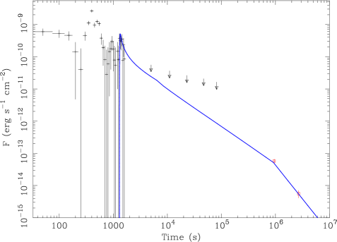
Figure 13: X–ray light curve for a jetted fireball expanding in an ISM with the origin of the time shifted to $t_{0}=1300s$. The model parameters are $E_{53}=0.03$, $\Gamma_{0}=130$, $n=5$, $\varepsilon_{e}=0.29$, $\varepsilon_{B}=8\cdot 10^{-5}$, $p=2.1$, and $T_{b}=8\cdot 10^{5}s$.

5 Broadband analysis of XRF 011030 afterglow data

No optical counterpart has been detected for XRF 011030. From among all the optical observations, we considered those performed by Vijay et al. (2001) and Rhoads et al. (2001) because they are the most constraining. The upper limits are R$>$21 (Vijay et al. 2001) and R$>$23.6 (Rhoads et al. 2001) at 0.3 and 2.7 days after the burst, respectively. We correct magnitudes for the reddening due to the absorption of our Galaxy, finding $R>$ 20.4 and $R>$ 23.1 (corresponding to an optical flux $F_{\nu,opt1}=1.79\times 10^{-28}$ erg cm^-2 s^-1 Hz^-1 and $F_{\nu,opt2}=1.69\times 10^{-29}$ erg cm^-2 s^-1 Hz^-1) for the two observations. In the radio band, Taylor et al. (2001) associated a transient source with a flux $F_{\nu,R}=1.81\times 10^{-27}$ erg cm^-2 s^-1 Hz^-1 about 10.5 days after the burst with XRF 011030.

For a jetted fireball expanding in an ISM, a solution that accounts for X–ray (Fig. 13), optical (Fig. 14), and radio (Fig. 15) is given by $E_{53}=0.03$, $\Gamma_{0}=130$, $n=5$, $\varepsilon_{e}=0.29$, $\varepsilon_{B}=8\cdot 10^{-5}$, $p=2.1$, and $T_{b}=8\cdot 10^{5}$ s. We show the optical and radio light curves corresponding to this set of model parameters in Figs, 14 and 15, respectively. We investigated how well the parameters are constrained, with particular regard to the density. The density is mostly constrained by the data below the cooling frequency, in this case optical and radio, and whether times are greater than about $10^{4}$ s (that is the time when a spectral break occurs), also X–ray data. After $10^{4}$ s, the emitted flux in the X–ray and optical band is given by (Panaitescu & Kumar 2000):

$$F_{\nu}\propto E_{53}^{(p+3)/4}n^{1/2}\varepsilon_{e,-1}^{p-1}\varepsilon_{B,-4}^{(p+1)/4}.$$ (9)

This same relation applies for the radio data because, at the time of the observation, the injection frequency $\nu_{i}$ is below or very near the observational frequency $\nu_{obs}$. Thus, the normalization of the light curve in one of the three observational bands also determines the normalization of the light curve in the other two bands. This causes the model parameters to be well-constrained.

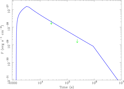
Figure 14: Optical light curve of a jetted fireball expanding in an ISM with the origin of the time shifted to $t_{0}=1300$ s. The model parameters are $E_{53}=0.03$, $\Gamma_{0}=130$, $n=5$, $\varepsilon_{e}=0.29$, $\varepsilon_{B}=8\cdot 10^{-5}$, $p=2.1$, and $T_{b}=8\cdot 10^{5}$ s.

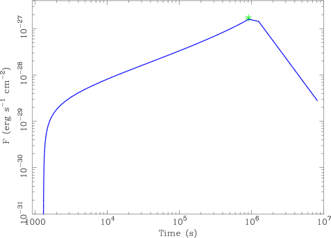
Figure 15: Radio light curve of a jetted fireball expanding in an ISM with the origin of the time shifted to $t_{0}=1300$ s. The model parameters are $E_{53}=0.03$, $\Gamma_{0}=130$, $n=5$, $\varepsilon_{e}=0.29$, $\varepsilon_{B}=8\cdot 10^{-5}$, $p=2.1$, and $T_{b}=8\cdot 10^{5}$ s.

In the case of the spherical fireball expanding in a wind, the break has to be self-consistently described (i.e., without the addition of a free parameter). Consequently, the model parameters are also well-constrained, $E_{53}=0.3$, $\Gamma_{0}=60$, $A_{*}=0.055$, $\varepsilon_{e}=0.02$, $\varepsilon_{B}=0.001$, and $p=2.1$. The corresponding X–ray, optical, and radio light curves are shown in Figs. 12, 16, and 17.

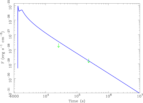
Figure 16: Optical light curve of a spherical fireball expanding in a wind with the origin of the time shifted to $t_{0}=1300$s. The model parameters are $E_{53}=0.3$, $\Gamma_{0}=60$, $A_{*}=0.055$, $\varepsilon_{e}=0.02$, $\varepsilon_{B}=0.001$, and $p=2.1$. We have assumed the efficiency in the conversion of the kinetic energy to be $\eta$=0.1.

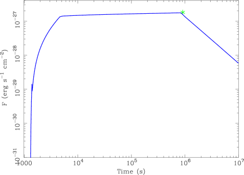
Figure 17: Radio light curve of a spherical fireball expanding in a wind with the origin of the time shifted to $t_{0}=1300$s. The model parameters are $E_{53}=0.3$, $\Gamma_{0}=60$, $A_{*}=0.055$, $\varepsilon_{e}=0.02$, $\varepsilon_{B}=0.001$, and $p=2.1$. We have assumed the efficiency in the conversion of the kinetic energy to be $\eta$=0.1.

6 Summary and conclusions

In this paper, we have presented the temporal and spectral analysis of the X-ray flash XRF 011030 observed by BeppoSAX. This event is one of the longest in the BeppoSAX sample (in’t Zand et al. 2002), with a duration of $\sim 1500$ s. In particular, along with the main pulse, we find a precursor event and a late X-ray flare.

While the spectrum of the main burst is not consistent with a black body, we cannot exclude this model for the precursor. This result could be due to the lower statistics available, but it is nonetheless interesting to note that, so far, there was only one example of a precursor consistent with such a model (Murakami et al. 1991). This feature could be associated with the cocoon formed by the jet emerging at the surface of the collapsing massive star (Ramirez-Ruiz et al. 2002; Waxman & Meszaros 2003).

After the launch of the Swift satellite, X–ray flares appear to be a common feature in GRBs light curves. This has favored the development of a large number of models to explain X–ray flares’ origin, both in internal and external shock scenarios (Zhang et al. 2006). X–ray flares observed by BeppoSAX in GRB 011121 and in XRR 011211 have spectra similar to that of the late afterglow. This similarity can be straightforwardly accounted for in the framework of the external shock, i.e., the flare represents the onset of the afterglow and it is connected with the late afterglow emission with a power law. For GRB 011121 and XRR 011211, a connection with the late afterglow is acceptable only by shifting the origin of the time $t_{0}$ to the instant of the flare (Piro et al. 2005). This implies a long duration engine activity (thick shell fireball, Sari & Piran (1999)).

We find that this scenario fits nicely with the observational data, including the X-ray flare and the late broadband radio, optical, and X-ray afterglow observations of XRF 011030 . The latter, performed by Chandra, indicate the presence of a temporal break occurring between $10^{4}$ s and $10^{6}$ s after the burst. We carried out a detailed modelling of the data, finding good agreement with observations for a spherical fireball expanding in a wind medium and for a jetted fireball expanding in an ISM. In the first case, the temporal break is explained by the passage of the cooling frequency in the X-ray band. We cannot exclude that the flare observed in XRF 011030 is due to internal shocks. However, this would require an engine activity that is tuned to track the peak energy of the emission during the prompt and flaring phases.

In the context of the external shock scenario, the time shift $t_{0}\sim 1300$ s is due to a long lasting central engine activity that remains active until the time of the flare, with the most of the energy released at the end of the emission phase (Sari & Piran 1999; Lazzati & Begelman 2006). In this case, the peak of the afterglow emission coincides with the flare, and the afterglow decay will be described by a self-similar solution by counting the time from the instant the inner engine turns off, i.e., when $t_{0}\simeq t_{eng}$.

We also find that a thin shell fireball cannot describe the flare in a continuous density profile, in fact, in this case, the flux rises and decays too slowly to describe the shape of the flare. Also, with a discontinuous density profile, it is very difficult to produce flares as high and narrow as that observed in XRF 011030, unless one assumes that the fireball is expanding in a clumpy medium (Dermer & Mitman 1999; Dermer 2005).

Recently, Swift observations have shown the presence of late X-ray flares in several other events. Some of these flares appear to have a spectral behaviour consistent with that of late X–ray flares observed by BeppoSAX, i.e., a soft spectrum substantially well-differentiated from the hard, prompt emission typically attributed to internal shocks (GRB 050126, GRB 050219a (Tagliaferri et al. 2005), and GRB 050904 (Burrows et al. 2005b)). GRB 050126 and GRB 050219a appear to follow a $(t-t_{0})^{-\alpha}$ power law, with $t_{0}\approx 100$ s, reasonably well. Instead in other flares, e.g XRF 050406 and GRB 050502B, the hardness ratio suggests a spectral evolution resembling the prompt emission (Burrows et al. 2005b). This behaviour has been thus interpreted by Burrows et al. (2005a) as due to internal shocks produced by a long duration central engine activity. However we notice that in some cases it could be possible explain hard-to-soft spectral evolution also in the context of the external shock scenario. When the fireball expands in a wind the cooling frequency $\nu_{c}$ increases with the time and there will be an instant when it enters in the X–ray band. At this instant the spectral index changes from $\beta=p/2$ to $\beta=(p-1)/2$ and the spectrum becomes harder of a factor 0.5.

Swift observations showed also the presence of multiple flares in GRB light curves on relatively small time scales, from $\sim$ 100 s up to $\sim$ 1000 s. For example GRB 050421 shows two successive flares within about 150 s (Godet et al. 2005), GRB 050607 has two flares within 500 s (Pagani et al. 2006) and GRB 050730 has three flares within 800 s (Burrows et al. 2005b). In these cases a thick shell fireball can be successful to explain only one of the flares appearing in the light curve, i.e. only one flare can be identified with the beginning of the afterglow emission. The other flares can be attributed to internal shocks or to the interaction with a clumpy medium in the framework of the external shock scenario. In conclusion we note that the present data suggest the existence of two categories of late X–ray flares differentiated by their spectral behaviour. It is also interesting to note that both in the framework of the internal shocks scenario and in that of external shocks, the explanation of late X–ray flares requires a central engine that remains active about until the time of the flare.