On the Determination of Neutrino Masses and Dark Energy Evolution from the Cross Correlation of CMB and LSS

Kazuhide Ichikawa and Tomo Takahashi

Institute for Cosmic Ray Research, University of Tokyo
Kashiwa 277-8582, Japan

We discuss the possibilities of the simultaneous determination of the neutrino masses and the evolution of dark energy from future cosmological observations such as cosmic microwave background (CMB), large scale structure (LSS) and the cross correlation between them. Recently it has been discussed that there is a degeneracy between the neutrino masses and the equation of state for dark energy. It is also known that there are some degeneracies among the parameters describing the dark energy evolution. We discuss the implications of these on the cross correlation of CMB with LSS in some details. Then we consider to what extent we can determine the neutrino masses and the dark energy evolution using the expected data from CMB, LSS and their cross correlation.

1 Introduction

Probing the masses of neutrinos has become one of the important targets in cosmology. Although neutrino oscillation experiments have well measured the mass differences as $\Delta m^{2}_{12}\simeq 7\times 10^{-5}~{}{\rm eV}^{2}$ from solar neutrino experiments [1, 2, 3, 4, 5, 6] and $\Delta m^{2}_{23}\simeq 2.6\times 10^{-3}~{}{\rm eV}^{2}$ from atmospheric neutrino experiments [7, 8], they are insensitive to the absolute values of the neutrino masses. Experiments using kinematical probe such as tritium decay measurements can give an upper bound on an absolute neutrino mass, however cosmology can give a more stringent bound. From the analyses of recent cosmological observations such as cosmic microwave background (CMB), large scale structure (LSS) and so on, we can conservatively say the current bound on the sum of neutrino masses $\sum m_{\nu}$ is around 2 eV (95% C.L.) [9, 10, 11, 12, 13, 14, 15].

Another important issue in cosmology is to understand the nature of dark energy. Almost all current cosmological observations suggest that the present universe is dominated by an enigmatic component called dark energy. Although many models for dark energy have been proposed so far, we have not pinned down the model yet. However, by parameterizing the dark energy with its equation of state $w_{X}$, cosmological observations can give the constraints on $w_{X}$. Assuming $w_{X}$ being constant, the current observations give $w_{X}\sim-1$ [9, 10, 11, 13, 14, 16, 17, 18]. Furthermore, even if we allow time-varying $w_{X}$ and/or non-flat universe, it is shown that $w_{X}$ is constrained to be around a cosmological constant for some types of time variation [19].

It has been shown that the constraint on the neutrino masses from CMB, LSS, type Ia Supernovae (SNeIa) and so on can be weakened if the equation of state for dark energy is allowed to take a value other than $-1$ and vice versa [20], which means that there is a degeneracy between the neutrino masses and the equation of state for dark energy. In Ref. [20], the equation of state for dark energy is assumed to be constant in time, however, most models of dark energy proposed so far have a time-varying equation of state. Importantly it should be noticed that there are degeneracies among parameters which describe the time dependence of dark energy equation of state. For example, it was discussed that, for the models with a constant equation of state $w_{X}$ and a time-varying equation of state parametrized as $w_{X}=w_{0}+(1-a)w_{1}$, there is a degeneracy between $w_{0}$ and $w_{1}$ in the CMB power spectrum and matter power spectrum [21]. Since now we know that neutrino has a mass and the equation of state for dark energy can have the time dependence, we should take both of them into account when we consider the constraints from observations. However, considering the degeneracies discussed above, we can expect that we encounter unfortunate situations when we want to determine the neutrino masses and the evolution of dark energy simultaneously.

In this paper, we discuss to what extent we can determine the neutrino masses and the evolution of dark energy, i.e., the time dependent equation of state, simultaneously from future cosmological observations. For this purpose, we make use of the Fisher matrix analysis using the expected data from future CMB and LSS observations. In addition to them, we also consider the cross correlation between CMB and LSS, which has been attracting attention of the community in recent years. In particular, we investigate the effect of the neutrino masses on the cross correlation, which has not been attempted previously in the literature. As is well known, after the universe has been dominated by dark energy, the gravitational potential decays, which drives the so-called late integrated Sachs-Wolfe (ISW) effect. Since the time-evolving gravitational potential that drives the ISW effect may also affect large scale structure formation, the temperature fluctuation from the ISW effect and the distribution of galaxy are considered to be correlated [22, 23, 24]. Since there is no ISW effect in the universe dominated by matter, the detections of the cross correlation of the ISW effect with galaxy survey is a piece of physical evidence for the existence of dark energy. The detection of the cross correlation between the WMAP temperature fluctuation and several galaxy surveys have been reported in Refs. [25, 26, 27, 28, 29, 30, 31, 32, 33, 34, 35]. Many authors have discussed the cross correlation of CMB with LSS to investigate the properties of dark energy and some other issues [21, 36, 37, 38, 39, 40, 41, 42]. In particular, it was shown that the cross correlation of CMB with galaxy survey can be a good probe for the evolution of dark energy [21].

The organization of this paper is as follows. In the next section, first we briefly discuss the degeneracy between the neutrino masses and the equation of state for dark energy and also that in models with the time-varying equation of state. Then, in section 3, we discuss the cross correlation of CMB with LSS and its spectra in scenarios with massive neutrinos and dark energy with some equations of state. In section 4, we study effects of massive neutrinos and dark energy on the suppression of growth of perturbation and the ISW effect and discuss how the masses of neutrinos and the equation of state for dark energy can affect the cross correlation spectrum. In section 5, we discuss a future constraint on the neutrino masses and the evolution of dark energy from CMB, LSS and the cross correlation of CMB and LSS. We give the summary of this paper in the final section.

2 Degeneracies in neutrino and dark energy sectors

In this section, we briefly discuss the degeneracy between the neutrino masses and the equation of state for dark energy $w_{X}$, which was recently pointed out [20] and also the degeneracy in the parameters which describe the time dependent $w_{X}$.

First we discuss the degeneracy between the neutrino masses and $w_{X}$. In Figs. 1 and 2, we show the CMB power spectra and matter power spectra respectively, for the cases with $\Lambda$CDM model and a model with massive neutrinos and the dark energy equation of state $w_{X}$ which is not equal to $-1$. For reference, we also plot the data from WMAP3 [13] in Fig. 1 and those from SDSS [14] in Fig. 2. For the $\Lambda$CDM model, we take the cosmological parameters as $\Omega_{m}h^{2}=0.13$, $\Omega_{b}h^{2}=0.023$, $h=0.735$, $\tau=0.09$ and $n_{s}=0.95$ which are the mean value of the power-law $\Lambda$CDM models from WMAP3. Here $\Omega_{i}$ is the energy density for a component $i$ ($i$ can be $b$, $m$ and $\nu$, which respectively stand for baryon, matter and neutrino) normalized by the critical energy density, $h$ is the Hubble parameter, $\tau$ is the reionization optical depth and $n_{s}$ is the scalar spectral index of primordial fluctuation. In this paper, we assume that the tensor mode is negligible. For the matter power spectra, we have corrected for a scale-dependent biasing following the treatment of Ref. [14]. This correction affects only the scales with $k\mathop{}_{\textstyle\sim}^{\textstyle>}0.07\,h\,$Mpc^-1. For the model with massive neutrinos and dark energy with $w_{X}\neq-1$, we take the cosmological parameters as $\Omega_{\nu}h^{2}=0.01$ and $w_{X}=-1.5$. Here we assume degenerate masses for 3 neutrino flavors and a constant $w_{X}$. The energy density and the masses of neutrinos are related by $\Omega_{\nu}h^{2}=\sum m_{\nu}/93.2\,{\rm eV}$. The other cosmological parameters are taken as $\Omega_{m}h^{2}=0.13$, $\Omega_{b}h^{2}=0.023$, $h=0.74$, $\tau=0.087$ and $n_{s}=0.94$. In general, dark energy component is characterized with its equation of state $w_{X}$ and speed of sound $c_{s}^{2}=\delta p_{X}/\delta\rho_{X}$. Although the background evolution depends on $w_{X}$ only, the fluctuation of dark energy depends on both $w_{X}$ and $c_{s}^{2}$. In this paper, we assume that $c_{s}^{2}=1$, which corresponds to the case with a scalar field dark energy, where $c_{s}^{2}$ is defined at the rest frame of the dark energy. As seen from the figure, these two parameter sets give almost the same spectra, which means that the values of $\chi^{2}$ from CMB and LSS are almost the same. As shown in Ref. [20], there is a degeneracy between $m_{\nu}$ and $w_{X}$ in the direction to the region where $w_{X}<-1$. This degeneracy can be explained as follows. To fit a model with massive neutrinos to large scale structure data, large $\Omega_{\nu}h^{2}$ can be compensated by increasing the energy density of matter. This cancellation seems not to be allowed because, assuming a flat universe and the cosmological constant for dark energy, SNeIa data constrain $\Omega_{m}$ to be $\sim 0.3$. However allowing the equation of state $w_{X}$ to vary, large values of $\Omega_{m}$ are consistent with observations of SNeIa with smaller $w_{X}$ [16]. This gives rise to the degeneracy in the matter power spectrum. As for CMB data, it is known that massive neutrinos affect the structure of acoustic peaks such as the position and the shape [12]. Increasing $\Omega_{\nu}h^{2}$, the peak position shifts to lower multipoles. However, by decreasing $w_{X}$, the position of the peak shifts to higher multipoles, which cancels the shift caused by increasing the value of $\Omega_{\nu}h^{2}$. Although the shape of the peaks is also slightly modified by increasing $\Omega_{\nu}h^{2}$, by changing other cosmological parameters, we can fit such a model to CMB data well. Thus by varying $w_{X}$, larger values of $\Omega_{\nu}h^{2}$ become to be allowed by the data.

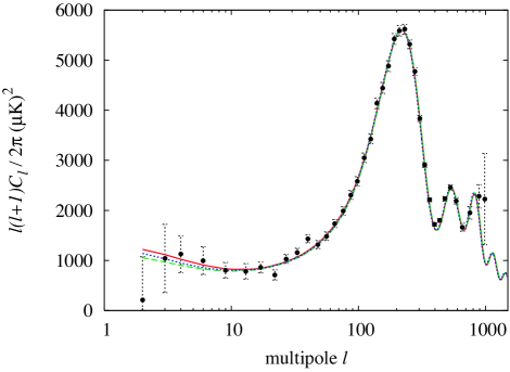
Figure 1: The CMB TT power spectrum for the $\Lambda$CDM model (red solid line), the model with $w_{X}=-1.5$ and $\Omega_{\nu}h^{2}=0.01$ (green dashed line) and the model with the time-varying equation of state $w_{0}=-1-1.2(1-a)$ and $\Omega_{\nu}h^{2}=0.01$ (blue dotted line). Notice that three lines are almost indistinguishable. The data from WMAP [13] are also plotted. For the cosmological parameters taken here, see the text.

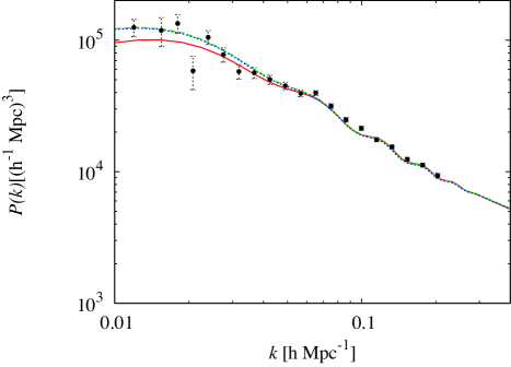
Figure 2: Matter power spectrum for the same models given in Fig. 1. The data from SDSS [14] are also plotted.

Next we discuss the degeneracy in models with dark energy with a time-varying equation of state. As mentioned above, most models of dark energy proposed so far such as quintessence have a time-dependent equation of state. Thus when we consider the constraints on the equation of state for dark energy $w_{X}$ phenomenologically, we should accommodate the time evolution of $w_{X}$ in some way. Although several ways have been proposed to include the time dependence of $w_{X}$, here we assume a simple form as [43, 44, 11]

$$w_{X}(a)=w_{0}+(1-a)w_{1}.$$ (2.1)

In Figs. 1 and 2, the CMB and matter power spectra for the cases with $w_{0}=-1$ and $w_{1}=-1.2$ are also plotted. Other cosmological parameters are taken to be the same as the case of a constant equation of state with massive neutrinos just above. As seen from the figure, the degeneracy in the CMB and LSS exists between the models with a constant $w_{X}$ and a time-varying $w_{X}$. The degeneracy comes from the fact that both models give almost the same angular diameter distance from last scattering surface which determines the positions of the acoustic peaks in the CMB angular power spectrum. Furthermore, the fluctuation of dark energy is almost irrelevant to the structure of the acoustic peaks , hence they give almost an identical power spectrum provided the angular diameter distances from last scattering surface are the same. A possible difference between the models with constant and time dependent $w_{X}$ is the ISW effect which affects the low multipole region. In fact, there is a small difference in the region, however, it is not enough to differentiate them due to the cosmic variance in this case.

Since there is a degeneracy between the neutrino masses and the constant equation of state for dark energy, we can expect that the situation becomes much worse when we also consider the time dependent dark energy equation of state. However, the possibility of differentiating the models with constant and time dependent $w_{X}$ using the cross correlation of CMB with LSS has been discussed [21]. Thus we may be able to break these degeneracies using the cross correlation. Before we discuss the future constraints on the masses of neutrino and dark energy evolution from CMB, LSS and their cross correlation, we study the effects of them on the cross correlation of CMB with LSS in the next section.

3 Cross correlation of CMB with galaxy

In this section, first we briefly review the formulation of the cross correlation of CMB with galaxies following Ref. [36]. Detailed descriptions of this issue can be found in Refs. [23, 24, 36].

The two point correlation function between the ISW signal and galaxy overdensity is defined as

$$C^{\rm ISW-g}(\theta)=\left\langle\Delta_{\rm ISW}(\hat{n}_{1})\delta_{\rm g}(\hat{n}_{2})\right\rangle,$$ (3.2)

where the angular brackets represent the ensemble average and $\cos\theta=\hat{n}_{1}\cdot\hat{n}_{2}$. $\Delta_{\rm ISW}$ is the temperature fluctuation from the ISW effect in the direction $\hat{n}_{1}$ which is written as

$$\Delta_{\rm ISW}(\hat{n}_{1})=\frac{\Delta T_{\rm ISW}}{T}=-2\int e^{-\tau(\eta)}\Phi^{\prime}(\hat{n}_{1},\eta)d\eta,$$ (3.3)

where $\eta$ is the conformal time and $e^{-\tau(\eta)}$ is the visibility function. Here a prime denotes the derivative with respect to the conformal time. $\Phi$ is the gravitational potential which appears in the metric perturbation in the conformal Newtonian gauge as

$$ds^{2}=-a^{2}(1+2\Phi)d\eta^{2}+a^{2}(1+2\Psi)dx^{2}.$$ (3.4)

Unless otherwise stated, we work in the conformal Newtonian gauge in this paper.

$\delta_{\rm g}(\hat{n}_{2})$ is the overdensity of galaxies in the direction $\hat{n}_{2}$.

$$\delta_{\rm g}(\vec{n}_{2})=\frac{n_{\rm g}(\vec{n}_{2})-\bar{n}_{\rm g}}{\bar{n}_{\rm g}},$$ (3.5)

where $\bar{n}_{\rm g}$ is the mean number density of galaxies. It is assumed that the galaxy number overdensity traces the density fluctuation of matter as

$$\delta_{\rm g}=b\delta_{\rm m},$$ (3.6)

where $b$ represents the galaxy bias. Thus $\delta_{\rm g}$ can be written as

$$\delta_{\rm g}(\hat{n}_{2})=b\int\phi(z)z^{\prime}\delta_{m}(\hat{n}_{2},\eta)d\eta,$$ (3.7)

where $\phi(z)$ is the selection function of a given galaxy survey.

As usual, it is convenient to decompose $C^{\rm ISW-g}(\theta)$ with the Legendre polynomials $P_{l}(\cos\theta)$ as

$$C^{\rm ISW-g}(\theta)=\sum_{l=2}^{\infty}\frac{2l+1}{4\pi}C_{l}^{\rm ISW-g}P_{l}(\cos\theta).$$ (3.8)

We subtracted the monopole and dipole contributions by construction. With the above definition, the cross-correlation power spectrum is given by

$$C^{\rm ISW-g}_{l}=4\pi\frac{9}{25}\int\frac{dk}{k}\Delta_{\mathcal{R}}^{2}I_{l}^{\rm ISW}(k)I_{l}^{\rm g}(k),$$ (3.9)

where $\Delta^{2}_{\mathcal{R}}$ is the primordial power spectrum. $I_{l}^{\rm ISW}(k)$ and $I_{l}^{\rm g}(k)$ are defined as

$$I_{l}^{\rm ISW}(k) = -2\int e^{-\tau(\eta)}\Phi^{\prime}_{k}(\eta)j_{l}[k(\eta_{0}-\eta)]d\eta,$$ (3.10)

$$I_{l}^{\rm g}(k) = b\int\phi(z)z^{\prime}\delta_{m}^{k}(\eta)j_{l}[k(\eta_{0}-\eta)]d\eta,$$ (3.11)

where the $j_{l}$ is the spherical Bessel function and $\eta_{0}$ is the conformal time at the present epoch. $\Phi_{k}$ and $\delta_{m}^{k}$ are the Fourier component of the gravitational potential and density fluctuation of matter which can be written as

$$\Phi(r\hat{n}) = \int\frac{d^{3}k}{(2\pi)^{3}}\Phi_{k}(\hat{n})e^{i\vec{k}\cdot\hat{n}r},$$ (3.12)

$$\delta_{m}(r\hat{n}) = \int\frac{d^{3}k}{(2\pi)^{3}}\delta_{m}^{k}(\hat{n})e^{i\vec{k}\cdot\hat{n}r},$$ (3.13)

where $r\equiv\eta_{0}-\eta$. For the later use, we also write down here the galaxy-galaxy correlation function which is given as

$$\omega_{l}^{(i,j)}=4\pi\frac{9}{25}\int\frac{dk}{k}\Delta_{\mathcal{R}}^{2}I_{l}^{\rm g(i)}(k)I_{l}^{\rm g(j)}(k),$$ (3.14)

where indices $(i,j)$ represent the redshift bins for the galaxy selection functions.

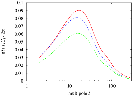
Figure 3: The cross correlation power spectrum for the same models given in Fig. 1.

Now we show the cross correlation spectrum in models introduced in the previous section. We computed the cross correlation spectra using the modified version of CMBFAST [45]. In Fig. 3, we plot the cross correlation power spectrum for the same models as those in Fig. 1. Here we use the normalized Gaussian selection function with the peak at redshift $\bar{z}=0.5$ and the variance $\sigma_{z}=0.07$. The other cosmological parameters are the same as those in Fig. 1. In the figure, the scalar amplitudes are normalized to the WMAP best fit values and the bias factors are determined by the fit to SDSS data. We will investigate in Sec. 5 whether or not the difference seen in Fig. 3 can be probed by future cross-correlation data. Before that, in the next section, we investigate the cross correlation in detail, discussing the suppression of matter fluctuation and the ISW effect in models with massive neutrinos and dark energy with some equations of state.

4 Suppression of perturbation growth and the ISW effect

In this section, we discuss the effects of massive neutrinos and dark energy with some equations of state on the suppression of fluctuation growth and the ISW effect. Below, the evolution of perturbation variables are calculated at the mode $k=0.01h$ Mpc^-1. Then we study the cross correlation spectrum in the models.

First we consider the effects of massive neutrinos on the suppression of fluctuation growth. Since massive neutrinos represent a smooth gravitationally stable component on small scales, they suppress the growth of matter fluctuation [46]. In linear regime, a small initial fluctuation $\delta_{0}$ grows as $\delta(a)=D(a)\delta_{0}$ where $D(a)$ is the growth factor. During matter-dominated universe, $D(a)$ grows as $D(a)\propto a$. An analytic formula for the growth factor is given in Ref. [46]. In Fig. 4, we show $\delta_{m}/a$ for the model with $\Omega_{\nu}h^{2}=0.01$ and $w_{X}=-1$ as a function of redshift. Other cosmological parameters are taken to be the same as those of the $\Lambda$CDM model in Fig. 1. We can see the suppression of growth of matter fluctuation in models with massive neutrinos. The growth of matter fluctuation is more suppressed by increasing the masses of neutrinos. To see the ISW effect in the model, we also plot $d\Phi/d\eta$ as a function of redshift in Fig. 5. As is clear from the figure, massive neutrinos have little effect on the evolution of the gravitational potential. Thus the mass of neutrinos is almost irrelevant to the late ISW effect, which means that we can expect that the neutrino masses have almost no effect on the cross correlation of CMB with LSS except for the overall suppression of matter fluctuation. Notice that, since we do not have much knowledge of the bias factor, we might not see such suppression.

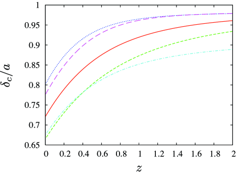
Figure 4: Suppression of fluctuation growth in models with dark energy equations of state $w_{X}=-1$ (red solid line), $w_{X}=-0.8$ (green short-dashed line), $w_{X}=-1.5$ (blue dotted line) and $w_{X}=-1-1.2(1-a)$ (purple long-dashed line). In these cases, we assume that $\Omega_{\nu}h^{2}=0$. The case with massive neutrinos $\Omega_{\nu}h^{2}=0.01$ and $w_{X}=-1$ (light blue dash-dotted line) is also plotted.

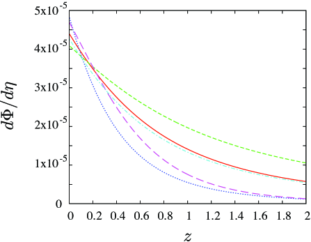
Figure 5: The derivative of the gravitational potential with respect to the conformal time for the same models given in Fig. 4.

Next we discuss the effects of dark energy on the suppression of fluctuation growth and the ISW effect. First we will discuss the suppression of fluctuation growth. The growth of matter fluctuation can be described by the following equation [47], including the fluctuation of dark energy

$$\delta_{c}{{}^{\prime\prime}}+\mathcal{H}\delta_{c}^{\prime}-\frac{3\mathcal{H}^{2}}{2}\Omega_{c}\delta_{c}=\frac{3\mathcal{H}^{2}}{2}\Omega_{X}\delta_{X},$$ (4.15)

where $\mathcal{H}=a^{\prime}/a$ is the conformal Hubble parameter, $\delta_{X}$ is the density perturbation of dark energy and $\Omega_{i}(z)=\rho_{i}(z)/\rho_{\rm total}(z)$ is the energy density of a component $i$ normalized by the total energy density at redshift $z$.

In Fig. 4, the fluctuations of matter for the cases with $w_{X}=-1.5,-1,-0.8$ and $w_{X}=-1-1.2(1-a)$ are shown. The matter fluctuation is more suppressed as increasing the value of $w_{X}$. This is due to the change of the background evolution by the domination of dark energy. The fluctuation of dark energy also affects the fluctuation of matter via gravity.

Another important effect of dark energy is the late ISW effect. As is well-known, when the universe is dominated by dark energy, the gravitational potential decays, which drives the late time ISW effect. The ISW effect can be written as

$$\Phi^{\prime}\sim\frac{1}{2k^{2}}\left[\mathcal{H}^{2}(\Omega_{m}\delta_{m}+\Omega_{X}\delta_{X})\right].$$ (4.16)

In Fig. 5, the evolutions of $\Phi^{\prime}$ as a function of redshift for several values of $w_{X}$ are shown. Increasing the values of $w_{X}$, the ISW effect is more enhanced at high redshift region, which leads to enhanced cross correlation power spectra. Notice that, at recent epoch, the values of $\Phi^{\prime}$ decreases as the values of $w_{X}$ increases. Thus the effects of $w_{X}$ can depend on the values of $w_{X}$ itself and also on the redshift.

Now we are in a position to discuss the cross correlation power spectrum for models with massive neutrinos and dark energy with some equations of state. In Fig. 6, we show the cross correlation power spectra for the cases with the constant equations of state ($w_{X}=-0.8,-1$ and $-1.5$) and the time-varying equation of state $w_{X}=-1-1.2(1-a)$. The case with $\Omega_{\nu}h^{2}=0.01$ and $w_{X}=-1$ is also plotted. We use the same galaxy selection function as that used in Fig. 3. Other cosmological parameters are taken to be the same as those of the $\Lambda$CDM model in Fig. 1. Since the masses of neutrinos suppress the growth of fluctuation, we can see the power spectrum of the cross correlation is also suppressed. Although the growth of matter fluctuation can also be suppressed in the dark energy dominated universe, effects of dark energy also come from the ISW effect. As the equation of state of the dark energy increases, the epoch where the energy density of dark energy dominates the universe becomes earlier than the case with the cosmological constant, which affects the evolution of the gravitational potential more at high redshift. Thus it can produce the large ISW signals. However, as mentioned above, the size of the ISW effect also depends on the epoch we consider. Thus the size of the cross correlation power spectrum depends on the values of $w_{X}$, its time dependence (i.e., $w_{1}$ in our parameterization) but also on the selection function.

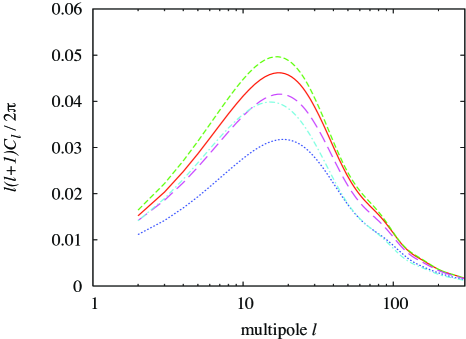
Figure 6: Cross-correlation power spectra for the same models given in Fig. 4.

5 Future constraints

Now we discuss attainable constraints on neutrino masses and the evolution of dark energy from future experiments of CMB, LSS and the cross correlation between them. We adopt the usual Fisher matrix method [48] for this purpose. The Fisher matrix is defined as

$$F_{\alpha\beta}=-\left\langle\frac{\partial^{2}\ln\mathcal{L}}{\partial\lambda_{\alpha}\partial\lambda_{\beta}}\right\rangle,$$ (5.17)

where $\mathcal{L}$ is the probability of observing a data set $\{x_{1},x_{2},...\}$ for a given cosmological parameter set $\{\lambda_{1},\lambda_{2},....\}$. Since there have been many works on the Fisher matrix analysis using future CMB and LSS data, we refer Refs. [49, 50, 51] for the details.

As for the cross correlation, here we briefly summarize the formulation following Ref. [21]. To forecast the errors in cosmological parameters, we use the expected CMB data from PLANCK [52] and the expected galaxy survey by Large Synoptic Survey Telescope (LSST) [53]. For PLANCK, we use the experimental specification which can be found in Ref. [54]. For the distribution of galaxies from a given survey, we assume that the total galaxy number is given by [38, 21],

$$n_{g}^{\rm total}(z)\propto z^{2}e^{-(z/z_{n})^{2}},$$ (5.18)

where $z_{n}$ is a parameters which gives a median redshift of the survey. The galaxies can be subdivided into multiple bins as

$$n^{\rm total}_{g}(z)=\sum_{i}n_{g}^{i}(z),$$ (5.19)

through photometric redshift. To approximate the redshift binning, we assume that photometric redshift estimates are Gaussian distributed with the variance of $\sigma(z)=\sigma_{\rm max}(1+z)/(1+z_{\rm max})$ [21]. Then the photometric redshift distributions are given by

$$n^{i}_{g}(z)=\frac{1}{2}n_{g}^{\rm tot}(z)\left[{\rm erfc}\left(\frac{z_{i-1}-z}{\sqrt{2}\sigma(z)}\right)-{\rm erfc}\left(\frac{z_{i}-z}{\sqrt{2}\sigma(z)}\right)\right],$$ (5.20)

where erfc is the complementary error function. For the LSST survey, we assume the galaxy survey sky coverage fraction as $f_{\rm sky}=0.5$ and 10 photometric redshift bins out to $z\sim 3$. The total galaxy number density is assumed to be $70$ gal/arcmin².

For the CMB-galaxy cross correlation, the Fisher matrix can be written as [21]

$$F_{\alpha\beta}^{\rm ISW-g}=f_{\rm sky}\sum_{l}(2l+1)\sum_{ij}\frac{\partial C^{\rm ISW-g}_{l(i)}}{\partial\lambda_{\alpha}}({\rm Cov}_{l})^{-1(i,j)}_{\rm ISW-g}\frac{\partial C^{\rm ISW-g}_{l(j)}}{\partial\lambda_{\beta}},$$ (5.21)

where the covariance matrix $({\rm Cov}_{l})_{\rm ISW-g}$ is given by

$$({\rm Cov}_{l})^{(i,j)}_{\rm ISW-g}=\tilde{C}^{TT}_{l}\tilde{\omega}^{(i,j)}_{l}+C^{\rm ISW-g}_{l(i)}C^{\rm ISW-g}_{l(j)}.$$ (5.22)

Here $\tilde{C}^{TT}_{l}$ is the observed spectrum which includes the noise

$$\tilde{C}^{TT}_{l}=C^{TT}_{l}+\sum_{C}\left[\left(\frac{\sigma_{C}\theta_{{\rm FWHM},C}}{T_{\rm CMB}}\right)^{-1}e^{l(l+1)\theta_{{\rm FWHM},C}/8\ln 2}\right]^{-1},$$ (5.23)

where $\sum_{C}$ represents the summation over channels. $\sigma_{C}$ and $\theta_{\rm FWHM,C}$ are the sensitivity per pixel and the width of the beam of a channel for a given measurement, respectively. $T_{\rm CMB}$ is the temperature of CMB. $\tilde{\omega}^{(i,j)}_{l}$ is the observed auto-correlation which is the sum of the signal and the Poisson noise

$$\tilde{\omega}^{(i,j)}_{l}=\omega^{(i,j)}_{l}+N_{l}^{(i,j)},$$ (5.24)

where $N_{l}^{(i,j)}$ is the Poisson noise which is uncorrelated between bins, thus

$$N_{l}^{(i,j)}=\frac{\delta_{ij}}{\bar{n}_{A}^{i}}.$$ (5.25)

$\bar{n}_{A}^{i}$ is the galaxy number per solid angle in the $i$-th bin. For the future constraints from CMB and LSS, we followed the method presented in Ref. [54].

Now we discuss attainable constraints from future experiments. As the fiducial model, we take the cosmological parameters as $\Omega_{b}h^{2}=0.024,\Omega_{m}h^{2}=0.14,\Omega_{X}=0.73,\tau=0.166$ and $n_{s}=0.99$. For the neutrino masses, we take $\sum m_{\nu}=0.3$ eV with the three degenerate masses. We checked that even if we assume the normal hierarchy with smaller neutrino masses, our conclusion does not change much. For the dark energy equation of state, we take $w_{X}=-1$ for the constant case and $w_{X}=-1+0.3(1-a)$ for the time dependent case. In Fig. 7, we plot the expected constraints on the neutrino masses and dark energy equation of state for the cases with the constant and the time dependent $w_{X}$ on the left and right panels respectively. When we obtain the constraints on the $\Omega_{\nu}h^{2}$ vs. $w_{0}$ plane, we marginalized over other cosmological parameters. Especially, for the latter case, we also marginalized over $w_{1}$ to obtain the constraint. In the figure, 1$\sigma$ C.L. contours are shown for the future data from CMB only, CMB$+$cross correlation, CMB$+$LSS, and all combined. As we can see, for the case with constant $w_{X}$, the cross correlation observations do not help much to constrain the neutrino masses and dark energy equation of state. However, for the case with the time-evolving dark energy equation of state, the cross correlation can be useful to determine the time evolution of $w_{X}$. As for the neutrino masses, the constraint on $m_{\nu}$ becomes weaker just a little in the case with the time evolving $w_{X}$. In both cases, the inclusion of LSS data can help to constrain the neutrino masses. As mentioned above, even if we assume the normal hierarchy for the neutrino masses, the shape and the size of the contours scarcely change. In fact, even if we marginalize over $w_{1}$, the constraint on the neutrino masses is not so weakened. This means that the time dependence of $w_{X}$ (i.e., $w_{1}$ in our parameterization) and $m_{\nu}$ are not strongly correlated.

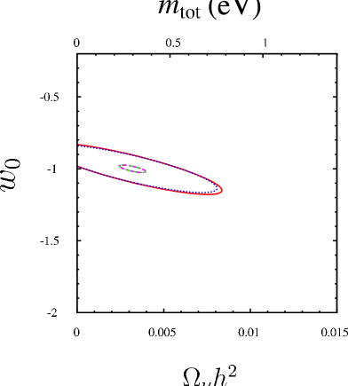
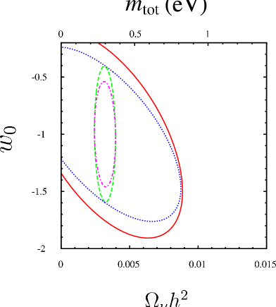
Figure 7: Expected 1$\sigma$ contours on the $\Omega_{\nu}h^{2}$ vs. $w_{0}$ plane. The cases with the constant $w_{X}$ (left) and time-varying $w_{X}$ (right) are shown. We marginalize $w_{1}$ for the latter case. Contours which correspond to the attainable future constraints from CMB only (red solid line), CMB$+$cross correlation (blue dotted line), CMB$+$LSS (green dashed line) and all combined (purple dash-dotted line) are shown.

Next we discuss the expected constraints on the dark energy evolutions, i.e., $w_{0}$ and $w_{1}$. In Fig. 8, we plot the future constraints on the time evolution of dark energy, fixing the neutrino masses (left panel) and marginalizing over the neutrino masses (right panel). As we can see, when we marginalize the masses of neutrinos, the uncertainty of $w_{0}$ and $w_{1}$ becomes larger, in particular, in the direction parallel to the $w_{0}$ axis. In fact, the constraint on $w_{1}$ is not weakened much compared to that on $w_{0}$. As mentioned above, this is because the masses of neutrino and $w_{1}$ are not so degenerate, which means that the time dependence of the equation of state for dark energy is not strongly correlated with the neutrino masses. It should also be noticed that the cross correlation of CMB with LSS can help to some extent to determine the evolution of dark energy even when we have uncertainties in the absolute values of the neutrino masses.

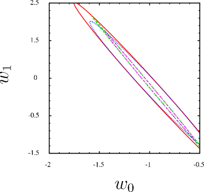
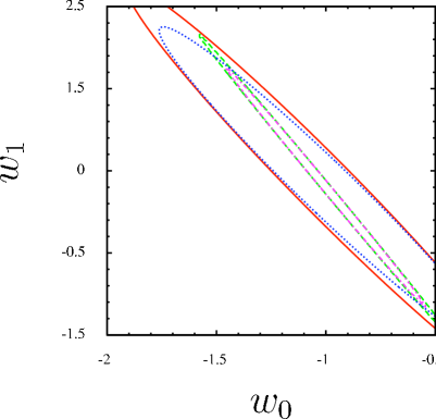
Figure 8: Expected 1$\sigma$ contours on the $w_{0}$ vs. $w_{1}$ plane. On the left panel, we fixed the neutrino masses to the fiducial value. On the right panel, we marginalized over the neutrino masses. Contours which correspond to the attainable future constraints from CMB only (red solid line), CMB$+$cross correlation (blue dotted line), CMB$+$LSS (green dashed line) and all combined (purple dash-dotted line) are shown.

6 Summary

We discussed the simultaneous determination of the neutrino masses and the evolution of dark energy from future cosmological observations. After presenting the degeneracies which exist between the neutrino masses and dark energy sectors, we considered the possibilities of breaking the degeneracies using the cross correlation of CMB and LSS. We studied the cross correlation power spectrum in those models in some details. We also discussed the suppression of perturbation growth and the ISW effect in the models. Then we presented the future constraints on the neutrino masses and the dark energy equation of state from the Fisher matrix analysis using the expected data from CMB, LSS and their cross correlation. First we showed the results on the $\Omega_{\nu}h^{2}$ vs. $w_{0}$ plane for the cases with a constant equation of state and a time-varying equation of state. We can see that the cross correlation of CMB with LSS can help to determine the time dependence of the equation of state to some extent. The constraint on the neutrino masses is not affected much since there is not strong correlation between the neutrino masses and $w_{1}$ which represents the time dependence of dark energy equation of state in our parameterization. Then we also discussed the constraints on the time evolution of equation of state, fixing and marginalizing the neutrino masses. When we marginalize the neutrino masses, the constraints on $w_{0}$ and $w_{1}$ are weakened. However, we showed that the cross correlation observation can be useful to determine the time evolution of the equation of state even if we do not have much information on the masses of neutrinos.

Note added: Recently the paper [55] appeared on the arXiv, which discusses the effect of the neutrino masses on the cross correlation. Also, Ref. [56] appeared more recently which has some overlaps with our analysis. Ref. [56] gives a qualitatively similar result to ours that the effects of the neutrino masses on the cross correlation are relatively small.

Acknowledgment: We acknowledge the use of CMBFAST [45] package for our numerical calculations. T.T. would like to thank the Japan Society for Promotion of Science for financial support.

References

- [1] B. T. Cleveland et al., Astrophys. J. 496, 505 (1998).
- [2] J. N. Abdurashitov et al. [SAGE Collaboration], Nucl. Phys. Proc. Suppl. 118, 39 (2003).
- [3] T. A. Kirsten [GNO Collaboration], Nucl. Phys. Proc. Suppl. 118, 33 (2003).
- [4] S. Fukuda et al. [Super-Kamiokande Collaboration], Phys. Rev. Lett. 86, 5656 (2001) [arXiv:hep-ex/0103033].
- [5] B. Aharmim et al. [SNO Collaboration], arXiv:nucl-ex/0502021.
- [6] T. Araki et al. [KamLAND Collaboration], Phys. Rev. Lett. 94, 081801 (2005) [arXiv:hep-ex/0406035].
- [7] Y. Fukuda et al. [Super-Kamiokande Collaboration], Phys. Rev. Lett. 81, 1562 (1998) [arXiv:hep-ex/9807003].
- [8] Y. Ashie et al. [Super-Kamiokande Collaboration], Phys. Rev. D 71, 112005 (2005) [arXiv:hep-ex/0501064].
- [9] D. N. Spergel et al. [WMAP Collaboration], Astrophys. J. Suppl. 148, 175 (2003) [arXiv:astro-ph/0302209].
- [10] M. Tegmark et al. [SDSS Collaboration], Phys. Rev. D 69, 103501 (2004) [arXiv:astro-ph/0310723].
- [11] U. Seljak et al., Phys. Rev. D 71, 103515 (2005) [arXiv:astro-ph/0407372].
- [12] K. Ichikawa, M. Fukugita and M. Kawasaki, Phys. Rev. D 71, 043001 (2005) [arXiv:astro-ph/0409768].
- [13] D. N. Spergel et al. [WMAP Collaboration], Astrophys. J. Suppl. 170, 377 (2007) [arXiv:astro-ph/0603449].
- [14] M. Tegmark et al., Phys. Rev. D 74, 123507 (2006) [arXiv:astro-ph/0608632].
- [15] S. Hannestad, JCAP 0305, 004 (2003) [arXiv:astro-ph/0303076]; V. Barger, D. Marfatia and A. Tregre, Phys. Lett. B 595, 55 (2004) [arXiv:hep-ph/0312065]; P. Crotty, J. Lesgourgues and S. Pastor, Phys. Rev. D 69, 123007 (2004) [arXiv:hep-ph/0402049]; G. L. Fogli, E. Lisi, A. Marrone, A. Melchiorri, A. Palazzo, P. Serra and J. Silk, Phys. Rev. D 70, 113003 (2004) [arXiv:hep-ph/0408045]; A. Goobar, S. Hannestad, E. Mortsell and H. Tu, JCAP 0606, 019 (2006) [arXiv:astro-ph/0602155]; G. Huetsi, Astron. Astrophys. 459, 375 (2006) [arXiv:astro-ph/0604129]; M. Fukugita, K. Ichikawa, M. Kawasaki and O. Lahav, Phys. Rev. D 74, 027302 (2006) [arXiv:astro-ph/0605362]; B. Feng, J. Q. Xia, J. Yokoyama, X. Zhang and G. B. Zhao, JCAP 0612, 011 (2006) [arXiv:astro-ph/0605742]; M. Cirelli and A. Strumia, JCAP 0612, 013 (2006) [arXiv:astro-ph/0607086]; S. Hannestad and G. G. Raffelt, JCAP 0611, 016 (2006) [arXiv:astro-ph/0607101]; G. L. Fogli et al., Phys. Rev. D 75, 053001 (2007) [arXiv:hep-ph/0608060]; C. Zunckel and P. G. Ferreira, JCAP 0708, 004 (2007) [arXiv:astro-ph/0610597]; J. R. Kristiansen, H. K. Eriksen and O. Elgaroy, Phys. Rev. D 74, 123005 (2006); J. R. Kristiansen, O. Elgaroy and H. Dahle, Phys. Rev. D 75, 083510 (2007);
- [16] J. L. Tonry et al. [Supernova Search Team Collaboration], Astrophys. J. 594, 1 (2003) [arXiv:astro-ph/0305008].
- [17] P. Astier et al. [The SNLS Collaboration], Astron. Astrophys. 447, 31 (2006) [arXiv:astro-ph/0510447]; A. G. Riess et al., arXiv:astro-ph/0611572. W. M. Wood-Vasey et al., arXiv:astro-ph/0701041; T. M. Davis et al., arXiv:astro-ph/0701510.
- [18] C. J. MacTavish et al., Astrophys. J. 647, 799 (2006) [arXiv:astro-ph/0507503].
- [19] K. Ichikawa and T. Takahashi, Phys. Rev. D 73, 083526 (2006) [arXiv:astro-ph/0511821]; K. Ichikawa, M. Kawasaki, T. Sekiguchi and T. Takahashi, JCAP 0612, 005 (2006) [arXiv:astro-ph/0605481]; K. Ichikawa and T. Takahashi, JCAP 0702, 001 (2007) [arXiv:astro-ph/0612739]; K. Ichikawa and T. Takahashi, arXiv:0710.3995 [astro-ph]; J. L. Crooks, J. O. Dunn, P. H. Frampton, H. R. Norton and T. Takahashi, Astropart. Phys. 20, 361 (2003) [arXiv:astro-ph/0305495]; Y. g. Gong and Y. Z. Zhang, Phys. Rev. D 72, 043518 (2005) [arXiv:astro-ph/0502262]; G. B. Zhao, J. Q. Xia, H. Li, C. Tao, J. M. Virey, Z. H. Zhu and X. Zhang, Phys. Lett. B 648, 8 (2007) [arXiv:astro-ph/0612728]; Y. Gong, Q. Wu and A. Wang, arXiv:0708.1817 [astro-ph]; D. Rapetti and S. W. Allen, arXiv:0710.0440 [astro-ph].
- [20] S. Hannestad, Phys. Rev. Lett. 95, 221301 (2005) [arXiv:astro-ph/0505551].
- [21] L. Pogosian, P. S. Corasaniti, C. Stephan-Otto, R. Crittenden and R. Nichol, Phys. Rev. D 72, 103519 (2005) [arXiv:astro-ph/0506396].
- [22] R. G. Crittenden and N. Turok, Phys. Rev. Lett. 76, 575 (1996) [arXiv:astro-ph/9510072].
- [23] H. V. Peiris and D. N. Spergel, Astrophys. J. 540, 605 (2000) [arXiv:astro-ph/0001393].
- [24] A. Cooray, Phys. Rev. D 65, 103510 (2002) [arXiv:astro-ph/0112408].
- [25] P. Fosalba and E. Gaztanaga, Mon. Not. Roy. Astron. Soc. 350, L37 (2004) [arXiv:astro-ph/0305468].
- [26] S. P. Boughn and R. G. Crittenden, Nature 247, 45 (2004).
- [27] S. P. Boughn and R. G. Crittenden, New Astron. Rev. 49, 75 (2005) [arXiv:astro-ph/0404470].
- [28] P. Fosalba and E. Gaztanaga Mon. Not. Roy. Astron. Soc. 350, 37 (2004).
- [29] P. Fosalba, E. Gaztanaga and F. Castander, Astrophys. J. 597, L89 (2003) [arXiv:astro-ph/0307249].
- [30] R. Scranton et al. [SDSS Collaboration], arXiv:astro-ph/0307335.
- [31] N. Afshordi, Y. S. Loh and M. A. Strauss, Phys. Rev. D 69, 083524 (2004) [arXiv:astro-ph/0308260].
- [32] N. Padmanabhan, C. M. Hirata, U. Seljak, D. Schlegel, J. Brinkmann and D. P. Schneider, Phys. Rev. D 72, 043525 (2005) [arXiv:astro-ph/0410360].
- [33] A. Cabre, E. Gaztanaga, M. Manera, P. Fosalba and F. Castander, Mon. Not. Roy. Astron. Soc. Lett. 372, L23 (2006) [arXiv:astro-ph/0603690].
- [34] T. Giannantonio et al., Phys. Rev. D 74, 063520 (2006) [arXiv:astro-ph/0607572].
- [35] J. D. McEwen, P. Vielva, M. P. Hobson, E. Martinez-Gonzalez and A. N. Lasenby, Mon. Not. Roy. Astron. Soc. 373, 1211 (2007) [arXiv:astro-ph/0602398].
- [36] J. Garriga, L. Pogosian and T. Vachaspati, Phys. Rev. D 69, 063511 (2004) [arXiv:astro-ph/0311412].
- [37] L. Pogosian, JCAP 0504, 015 (2005) [arXiv:astro-ph/0409059].
- [38] W. Hu and R. Scranton, Phys. Rev. D 70, 123002 (2004) [arXiv:astro-ph/0408456].
- [39] P. S. Corasaniti, T. Giannantonio and A. Melchiorri, Phys. Rev. D 71, 123521 (2005) [arXiv:astro-ph/0504115].
- [40] E. Gaztanaga, M. Manera and T. Multamaki, arXiv:astro-ph/0407022.
- [41] A. Cooray, P. S. Corasaniti, T. Giannantonio and A. Melchiorri, Phys. Rev. D 72, 023514 (2005) [arXiv:astro-ph/0504290].
- [42] N. Afshordi, Phys. Rev. D 70, 083536 (2004) [arXiv:astro-ph/0401166].
- [43] E. V. Linder, Phys. Rev. Lett. 90, 091301 (2003) [arXiv:astro-ph/0208512].
- [44] R. R. Caldwell, M. Doran, C. M. Mueller, G. Schaefer and C. Wetterich, Astrophys. J. 591, L75 (2003) [arXiv:astro-ph/0302505].
- [45] U. Seljak and M. Zaldarriaga, Astrophys. J. 469, 437 (1996) [arXiv:astro-ph/9603033].
- [46] W. Hu and D. J. Eisenstein, Astrophys. J. 498, 497 (1998) [arXiv:astro-ph/9710216].
- [47] R. Bean and O. Dore, Phys. Rev. D 69, 083503 (2004) [arXiv:astro-ph/0307100].
- [48] M. Tegmark, A. Taylor and A. Heavens, Astrophys. J. 480, 22 (1997) [arXiv:astro-ph/9603021].
- [49] G. Jungman, M. Kamionkowski, A. Kosowsky and D. N. Spergel, Phys. Rev. Lett. 76, 1007 (1996) [arXiv:astro-ph/9507080].
- [50] M. Tegmark, Phys. Rev. Lett. 79, 3806 (1997) [arXiv:astro-ph/9706198].
- [51] D. J. Eisenstein, W. Hu and M. Tegmark, Astrophys. J. 518, 2 (1998) [arXiv:astro-ph/9807130].
- [52] http://www.rssd.esa.int/Planck
- [53] http://www.lsst.org/
- [54] J. Lesgourgues, S. Pastor and L. Perotto, Phys. Rev. D 70, 045016 (2004) [arXiv:hep-ph/0403296].
- [55] A. Kiakotou, O. Elgaroy and O. Lahav, arXiv:0709.0253 [astro-ph].
- [56] J. Lesgourgues, W. Valkenburg and E. Gaztanaga, arXiv:0710.5525 [astro-ph].