Photoionized H$\beta$ Emission in NGC 5548: It Breathes!

Abstract

Emission-line regions in active galactic nuclei and other photoionized nebulae should become larger in size when the ionizing luminosity increases. This “breathing” effect is observed for the H$\beta$ emission in NGC 5548 by using H$\beta$ and optical continuum lightcurves from the 13-year 1989-2001 AGN Watch monitoring campaign. To model the breathing, we use two methods to fit the observed lightcurves in detail: (i) parameterized models and, (ii) the MEMECHO reverberation mapping code. Our models assume that optical continuum variations track the ionizing radiation, and that the H$\beta$ variations respond with time delays $\tau$ due to light travel time. By fitting the data using a delay map $\Psi(\tau,F_{c})$ that is allowed to change with continuum flux $F_{c}$, we find that the strength of the H$\beta$ response decreases and the time delay increases with ionizing luminosity. The parameterized breathing models allow the time delay and the H$\beta$ flux to depend on the continuum flux so that, $\tau\propto F_{c}^{\beta}$ and $F_{H\beta}\propto F_{c}^{\alpha}$. Our fits give $0.1<\beta<0.46$ and $0.57<\alpha<0.66$. $\alpha$ is consistent with previous work by Gilbert & Peterson (2003) and Goad, Korista & Knigge (2004). Although we find $\beta$ to be flatter than previously determined by Peterson et al. (2002) using cross-correlation methods, it is closer to the predicted values from recent theoretical work by Korista & Goad (2004).

1 Introduction

Photoionization models predict the sizes of Strömgren zones for H II regions and planetary nebulae ionized by hot stars of various luminosities and spectral types. Higher luminosity can maintain a larger mass of ionized gas. Dynamical tests of photoionization models are rare. The ionizing stars evolve in luminosity at rates too slow for humans to directly observe changes in radius. However, active galacic nuclei (AGN) vary on much shorter time-scales (days to months). Rapid variations in the ionizing luminosity emerging from an AGN should cause the photoionized region to expand and contract. This ‘breathing’ of the emission-line region is an interesting test of photoionization models.

Although the time-scales of the variations are convenient to human observers, unfortunately, the angular sizes of the broad emission-line regions are too small to be resolved directly. A nebula 100 light days across at a distance of 100 Mpc spans only 180 micro-arcseconds. Fortunately, light travel times within the nebula introduce time delays for any changes in the line emission. The ionizing radiation from the innermost regions of an AGN is reprocessed by gas in the surrounding broad line region (BLR). As the central source varies, spherical waves of heating and ionization, cooling and recombination, expand at the speed of light through the BLR. A change in ionization causes a corresponding change in the reprocessed emission. In AGNs, the recombination timescales of the gas in the BLR is very short compared to the light travel time, so the delay seen by a distant observer is dominated by the light travel time. Hence, we see line emission correlated with the continuum but with a time delay, $\tau$. A gas cloud 1 light day behind the ionizing source will be seen to brighten 2 days after the ionizing source flux rises. Thus, we can use light travel time delays to measure the size of the region that is responding to variations in the ionizing flux, where the reverberation radius is $\langle R\rangle\approx\langle\tau\rangle c$. Echo mapping, or reverberation mapping (Blandford & McKee, 1982), aims to use this correlated variability to determine the kinematics and structure of the BLR, as well as the mass of the central supermassive black hole (e.g. Peterson, 1993; Peterson et al., 2004, and references therein).

The nearby ($z=0.017$) Seyfert 1 galaxy NGC 5548 has been intensively monitored in the optical range for 13 years (1989-2001) by the international AGN Watch consortium (e.g. Peterson et al., 2002). Those data spanning the source in a wide range of luminosity states are ideal for searching for this ‘breathing’ effect. In this paper, we investigate the luminosity dependence of the H$\beta$ emission and present two methods of fitting the data, accounting for the ‘breathing’ using (i) parameterized models and (ii) the reverberation mapping code MEMECHO (Horne, Welsh & Peterson, 1991; Horne, 1994). Although previous work by Peterson et al. (1999, 2002); Gilbert & Peterson (2003); Goad et al. (2004) has studied the luminosity dependence of the H$\beta$ emission in NGC 5548, this study applies alternative techniques to characterise the ‘breathing’. In $\S$2 we describe the echo mapping techinque and discuss the luminosity dependence of the emission-line lightcurve. In $\S$3 we present the luminosity dependent parameterized models followed by the MEMECHO method in $\S$4. The results of these methods of fitting the data, and their implications, are discussed in $\S$5 and we summarize our main findings in $\S$6.

2 Echo Mapping

The emission line flux, $F_{l}(t)$, that we see at each time, $t$, is driven by the continuum variations, $F_{c}(t)$, and arises from a range of time delays, $\tau$. The emission line lightcurve is therefore a delayed and blurred version of the continuum lightcurve. In the usual linearized echo model the line lightcurve is modelled as

$$F_{c}(t)=\bar{F_{c}}+\Delta F_{c}(t)$$ (1)

$$F_{l}(t)=\bar{F_{l}}+\int_{0}^{\tau_{\rm max}}\Psi\left(\tau\right)\Delta F_{c}(t-\tau)d\tau\ .$$ (2)

where $\Psi(\tau)$ is the transfer function, or delay map. We can adopt a continuum background level $\bar{F_{c}}$, somewhat arbitrarily, at the median of the observed continuum fluxes. $\bar{F_{l}}$ is then a constant background line flux that would be produced if the continuum level were constant at $\bar{F_{c}}$.

A simple way of determining the size of the emission-line region is to determine the time delay (or ‘lag’) between the line and continuum lightcurves using cross-correlation. Taking the centroid of the cross-correlation function (CCF) as the lag gives a luminosity-weighted radius for the BLR (Robinson & Perez, 1990). However, the cross-correlation function is a convolution of the delay map, $\Psi(\tau)$, with the auto-correlation function (ACF) of the driving continuum lightcurve. It is therefore possible that changes in the measured cross-correlation lag arise from changes in the continuum auto-correlation function rather than in the delay map (e.g. Robinson & Perez, 1990; Perez, Robinson & de La Fuente, 1992; Welsh, 1999). If the continuum variations become slower, a sharp peak at low time-delay in the delay distribution will be blurred by the broader auto-correlation function and the peak of the cross-correlation function will be shifted to larger delays (Netzer & Maoz, 1990). A typical delay map may have a rapid rise to a peak at small lag, and a long tail to large lags. The asymmetric peak in $\Psi(\tau)$, will shift toward its longer wing when blurred by the auto-correlation function. Thus the lag measured by cross-correlation analysis depends not only on the delay distribution, $\Psi\left(\tau\right)$, but also on the characteristics (ACF) of the continuum variations.

Previous analysis of the AGN Watch data for NGC 5548 by Peterson et al. (2002) determined the H$\beta$ emission-line lag relative to the optical continuum, on a year by year basis, using cross-correlation. These authors find that the lag increases with increasing mean continuum flux. To improve upon the CCF analysis we use the echo mapping technique to fit the lightcurves in detail. However, the linearized echo model (Eq. 2) is appropriate only when the delay map is independent of time (static). In this paper we extend the model to search for changes in the delay map with luminosity.

2.1 Luminosity-Dependent Delay Map

The above linearized echo model (Eq. 2) assumes that the line emissivity and continuum flux can be related by a linear function and thus is appropriate only for responses that are static. In principle, the delay map may change with time, for example, due to motion, or changes in quantity, of line-emitting gas within the system. The delay map may also change with luminosity. In the “local optimally emitting clouds” (LOC) model (Baldwin et al., 1995) at each time delay there is a variety of gas clouds with differing properties, and those most efficient at reprocessing tend to dominate the line flux emerging from the region. A change in ionizing luminosity induces a change in the efficiency of reprocessing at each place in the region and so the time delay at which the line emission is dominant will change. When a cloud is partially ionized its response may initally be large so that increasing luminosity increases the depth of the ionized zone on the face of the cloud. Once the cloud becomes completely ionized, however, further increases in ionizing flux are less effectively reprocessed. The line flux saturates, and may even decrease with increasing ionizing flux due to either ionization or decline in the recombination coefficients caused by an increase in gas temperature (O’Brien, Goad & Gondhalekar, 1995).

To account for these effects, we generalise the echo model by allowing the delay map to be luminosity-dependent, $\Psi(\tau,F_{c})$. The response we see at time $t$ from a parcel of emission-line gas located at time delay $\tau$ is set by the luminosity of the nucleus that we saw at the earlier time $t-\tau$. Thus,

$$F_{l}(t)=\bar{F_{l}}+\int_{0}^{\tau_{\rm max}}\Psi\left[\tau,F_{c}(t-\tau)\right]\Delta F_{c}(t-\tau)d\tau\ .$$ (3)

2.2 Luminosity dependence of H$\beta$ flux

A well-established correlation between continuum and emission-line properties is the ‘Baldwin’ effect (Baldwin, 1977; Osmer, Porter & Green, 1994) where, in different AGN, broad emission-line equivalent width is observed to decrease with increasing continuum level. The relationship between the line luminosity, $L_{l}$, and the continuum luminosity, $L_{c}$, can be described by

$$L_{l}\propto L_{c}^{\alpha}\ .$$ (4)

Kinney, Rivolo & Koratkar (1990) find that $\alpha\approx 0.83$ for C$IV$, and $\alpha\approx 0.88$ for Ly$\alpha$.

Within a single source, various studies have shown that emission lines have a nonlinear response to continuum variations (e.g. Pogge & Peterson, 1992; Dietrich & Kollatschny, 1995). This ‘intrinsic Baldwin effect’ (Kinney et al., 1990; Krolik et al., 1991; Pogge & Peterson, 1992; Korista & Goad, 2004) where the H$\beta$ emission-line response to variations in the continuum decreases with increasing continuum level has been observed for NGC 5548 (Gilbert & Peterson, 2003; Goad, Korista & Knigge, 2004). In terms of the continuum flux, $F_{c}$, and the line flux, $F_{l}$, the intrinsic Baldwin effect is described by

$$F_{l}\propto F_{c}^{\alpha}\ .$$ (5)

This nonlinearity can be seen by simply examining the 13-year lightcurves (Fig. 1). In the lowest state (1992), the trough in the H$\beta$ lightcurve is deeper than in the continuum lightcurve, whereas in the highest state (1998), the H$\beta$ peak is not as pronounced as the continuum. This argument neglects that light travel time delay smears out the emission-line response, but this should happen to both the peak and the trough.

The relation between the optical continuum flux at 5100$\mathrm{\AA}$ and the H$\beta$ line flux is examined in Fig. 2 (a), where a power-law (Eq. 5) with $\alpha=0.63$ gives a good fit. Here we corrected the optical continuum flux at 5100 $\mathrm{\AA}$, $F_{opt}$, for the background host galaxy contribution, $F_{gal}$, where we take $F_{gal}=3.4\times 10^{-15}$ erg s^-1 cm^-2 $\mathrm{\AA}^{-1}$ as determined by Romanishin et al. (1995). The narrow-line component of the H$\beta$ line has also been removed, and we use $F_{H\beta}(narrow)=6.7\times 10^{-14}$ erg s^-1 cm^-2 determined by Gilbert & Peterson (2003). We included a time delay of 17.5 days between the continuum flux and H$\beta$ flux to remove reverberation effects which was determined by cross-correlation of the full 13-year lightcurves. This time delay was subtracted from the times of each of the H$\beta$ data points and the continuum flux at this new time determined via linear interpolation. Gilbert & Peterson (2003) do a more detailed analysis allowing for the different time delays observed each year, and when adopting the same galaxy continuum background and H$\beta$ narrow-line component, determine $\alpha=0.65\pm 0.02$. Goad et al. (2004) find that the slope of this relation is not constant, but decreases as the continuum flux increases, an effect which is predicted by the photoionization models of Korista & Goad (2004). However, the driving ionizing continuum maybe closer to that observed in the UV at 1350 $\mathrm{\AA}$, and so previous observations of NGC 5548 at this wavelength by the AGN Watch using IUE and HST (Clavel et al., 1991; Korista et al., 1995) can be used to correct the relationships determined by the optical continuum. Using the IUE data Peterson et al. (2002) finds a relation $F_{opt}\propto F_{UV}^{0.56}$, while Gilbert & Peterson (2003) find a relation of $F_{opt}\propto F_{UV}^{0.67}$. Combining both IUE and HST data, we find a relation $F_{opt}\propto F_{UV}^{0.53\pm 0.02}$ (see Fig. 2 (b)) assuming no time delay between the optical and UV continuum and linearly interpolating to get the optical continuum at the required times. From this result, we get a relationship between the H$\beta$ flux and the ionizing UV flux of $F_{H\beta}\propto F_{UV}^{0.31}$. However, the UV flux can be combined directly with the $H\beta$ flux to determine this relationship. Including cross-correlation time delays for the relavent years (19.7 days for the 1989 data and 13.6 days for the 1993 data), we determine this relation directly to be $F_{H\beta}\propto F_{UV}^{0.26\pm 0.01}$ (see Fig. 2 (c)).

Figure 1: Lightcurves for optical continuum flux ($10^{-15}$ erg s^-1 cm${}^{-2}\rm{\AA}^{-1}$, at 5100 $\rm{\AA}$) and H$\beta$ emission line flux ($10^{-13}$ erg s^-1 cm^-2) from the 1989-2001 AGN Watch data on NGC 5548. LS and HS marks the lowest (1992) and highest (1998) states of the lightcurves respectively. Solid lines mark the galaxy contribution to the continuum flux (Romanishin et al., 1995) and the narrow-line contribution to the H$\beta$ flux (Gilbert & Peterson, 2003). Dashed lines separate the observing seasons.

Figure 2: (a) Narrow-line subtracted H$\beta$ flux vs. optical continuum flux at 5100$\mathrm{\AA}$ ($F_{opt}$), with the host galaxy continuum flux removed ($F_{gal}$ ) for the 13-year data set. The solid line indicates $F_{H\beta}\propto F_{opt}^{0.63}$. A time delay between the continuum and H$\beta$ fluxes of 17.5 days is included. (b) UV continuum flux at 1350$\mathrm{\AA}$ vs. $F_{opt}$ - $F_{gal}$. UV data are taken from the IUE campaigns in 1989 (circles; Clavel et al., 1991) and 1993 (squares) as well as the HST campaign in 1993 (triangles; Korista et al., 1995). The solid line indicates the best fit of $F_{opt}\propto F_{UV}^{0.53\pm 0.02}$. (c) Narrow-line subtracted H$\beta$ flux vs. UV continuum flux at 1350$\mathrm{\AA}$ (symbols as in (b)). A time delay between the H$\beta$ and UV fluxes has been added with the H$\beta$ fluxes from 1989 19.7 days behind the UV and for the 1993 data the delay is 13.6 days. The solid line indicates the best fit of $F_{H\beta}\propto F_{UV}^{0.28\pm 0.01}$.

2.3 Luminosity dependence of time delay

As the ionizing luminosity varies we expect the size of the photoionized region to expand and contract - a larger luminosity should ionize gas to a greater distance. We now consider a couple of simple theoretical predictions for this effect. If the BLR acts as a simple Strömgren sphere with uniform gas density, then one would predict that $R\propto L^{1/3}$. If instead we assume that the response in an emission line will be greatest at some density, $n$, and ionization parameter, $\Gamma\propto L/R^{2}n$, then it is easy to show this predicts $R\propto L^{1/2}$ (for a particular value of the product $\Gamma n$) (Peterson et al., 2002). More detailed photoionization modeling (using the LOC model) by Korista & Goad (2004) predicts a responsivity-weighted radius scaling as $R\propto L^{0.23}$ for H$\beta$. Photoionization models by O’Brien et al. (1995) and also Korista & Goad (2004) both come to the conclusion that a relationship between emission-line lag and incident continuum level is due to a non-linear emission-line response.

Peterson et al. (1999) and more recently Peterson et al. (2002) used a year by year cross-correlation analysis of the AGN Watch data for NGC 5548 to show that the H$\beta$ emission-line lag (relative to the optical continuum) is correlated with the mean optical continuum flux (at 5100$\rm{\AA}$). As the mean optical continuum flux increases, the lag, and hence the size of the H$\beta$ emitting region, is seen to increase. Using the full 13-year lightcurves for NGC 5548, Peterson et al. (2002) find $\tau\propto F_{opt}^{0.95}$, though with much scatter. They argue, however, that the UV continuum (at 1350$\rm{\AA}$) is much closer to the driving ionizing continuum than the optical continuum used. Correcting for the relationship between the optical and UV continuum (using $F_{opt}\propto F_{UV}^{0.53}$) leads to $\tau\propto F_{UV}^{0.50}$ as predicted assuming that the emission will be greatest at some particular gas density and ionization parameter.

To test the predictions, using more complex methods than the cross-correlation, we have fitted the data allowing for these breathing effects. Firstly, we present our parameterized models and then the MEMECHO fits to the 13-year (1989-2001) AGN Watch optical continuum and H$\beta$ lightcurves for NGC 5548 before discussing these results, their findings and implications.

3 Parameterized models

In this method we model the delay map and include parameters to allow it to be luminosity dependent. We choose to model the delay map as a Gaussian in $\ln\tau$,

$$\Psi\left(\tau\right)=\frac{\Psi_{0}}{A}\exp\left(-\frac{1}{2}\left[\frac{\ln(\tau/\tau_{0})}{\Delta\ln\tau}\right]^{2}\right)$$ (6)

where $\tau_{0}$ is the peak of the Gaussian and $\Delta\ln\tau$ is the width of the Gaussian. $\Psi_{0}$ scales the strength of the delay map. We include a normalisation factor, $1/A$, chosen so that $\Psi_{0}=\int\Psi\left(\tau\right)d\tau$, where,

$$A = \int_{0}^{\infty}\exp\left(-\frac{1}{2}\left[\frac{\ln(\tau/\tau_{0})}{\Delta\ln\tau}\right]^{2}\right)d\tau$$ (7)

$$= \sqrt{2\pi}\,(\Delta\ln\tau)\,\tau_{0}\,\exp\left[(\Delta\ln\tau)^{2}/2\right]\ .$$

We select this model as it ensures causality ($\Psi\left(\tau\right)=0$ for $\tau<0$) while allowing parameters $\tau_{0}$ and $\Delta\ln\tau$ to control the centroid and width of the delay distribution.

We introduce three ‘breathing’ parameters to allow the delay map to be luminosity dependent. To account for the two effects discussed in $\S$2.2 and $\S$2.3, we introduce $\alpha$ to model the ‘intrinsic Baldwin effect’, so that $F_{H\beta}\propto F_{opt}^{\alpha}$, and $\beta$ to allow the mean time delay of the delay map to depend on the continuum flux i.e., $\tau\propto F_{opt}^{\beta}$. A further parameter, $\gamma$, is introduced to allow the width of the delay map, $\Delta\ln\tau$, to depend on the continuum flux, so that $\Delta\ln\tau\propto F_{opt}^{\gamma}$. Fig. 3 illustrates how these parameters affect the delay map as the continuum flux increases. A linear line response corresponds to $\alpha=1.0$, whereas $\beta=0.0$ means that there is no dependence of time-delay with luminosity, and $\gamma=0.0$ ensures $\Delta\ln\tau$ is constant. A positive value for $\beta$ indicates that the time delay is increasing with increasing continuum flux, and similarly, a positive value for $\gamma$ indicates that the width of the delay map is increasing with increasing continuum flux.

Figure 3: Delay maps for different values of the ‘breathing’ parameters $\alpha$, $\beta$ and $\gamma$. Different lines indicate different continuum fluxes where $F_{opt}$ = 5.0 (solid), 10.0 (dashed), 15.0 (dot-dashed) and 20.0 (dotted) $\times 10^{-15}$ erg s^-1 cm^-2 $\mathrm{\AA}^{-1}$. $\overline{\tau_{0}}=17.5$ days and $\overline{\Delta\ln\tau}=0.3$ throughout.

One complication is the host galaxy’s contribution, $F_{gal}$, to the observed optical continuum flux $F_{opt}(t)$. We treat this by defining the normalised lightcurve (with the background galaxy contribution subtracted) as

$$X(t)=\frac{F_{opt}(t)-F_{gal}}{\overline{F_{opt}}-F_{gal}},$$ (8)

where $F_{gal}$ is the background galaxy continuum flux and $\overline{F_{opt}}$ is the mean continuum flux, so that $X=1$ when $F_{opt}=\overline{F_{opt}}$, and $X=0$ when $F_{opt}=F_{gal}$. In all fits we adopt a background galaxy continuum flux, $F_{gal}=3.4\times 10^{-15}$ erg s^-1 cm^-2 $\mathrm{\AA}^{-1}$ as determined by Romanishin et al. (1995).

We include the three ‘breathing’ parameters ($\alpha$, $\beta$ and $\gamma$) to our model as follows,

$$\Psi_{0} = \overline{\Psi_{0}}~{}\left[X(t-\tau)\right]^{\alpha-1}$$ (9)

$$\tau_{0} = \overline{\tau_{0}}~{}\left[X(t-\tau)\right]^{\beta}$$ (10)

$$\Delta\ln\tau = \overline{\Delta\ln\tau}~{}\left[X(t-\tau)\right]^{\gamma}\ .$$ (11)

where $\overline{\Psi_{0}}$, $\overline{\tau_{0}}$ and $\overline{\Delta\ln\tau}$ are just the values of $\Psi_{0}$, $\tau_{0}$ and $\Delta\ln\tau$ at the mean optical continuum flux, $\overline{F_{opt}}$. The H$\beta$ lightcurve is then just given by

$$F_{H\beta}(t)=\overline{F_{H\beta}}+\int_{0}^{\tau_{\rm max}}\Psi\left[\tau,X(t-\tau)\right]\Delta F_{opt}(t-\tau)d\tau\ ,$$ (12)

where,

$$F_{opt}(t)=\overline{F_{opt}}+\Delta F_{opt}(t)$$ (13)

As the delay map is Gaussian in $\ln\tau$, not $\tau$, the delay map is asymmetric and has a long tail to high time delays (unless $\Delta\ln\tau\ll 1$). Although we have parameterized the delay map in terms of $\tau_{0}$, the lag at which the delay map peaks, it is useful to characterise the delay map in terms of the median lag, $\tau_{med}$, and the mean lag, $\langle\tau\rangle$, as these values are more directly comparable to the cross-correlation lags. We define these quantities as

$$\frac{1}{2}=\frac{\int_{0}^{\tau_{med}}\Psi\left(\tau\right)d\tau}{\int_{0}^{\infty}\Psi\left(\tau\right)d\tau}\ ,$$ (14)

and

$$\langle\tau\rangle=\frac{\int_{0}^{\infty}\tau\Psi\left(\tau\right)d\tau}{\int_{0}^{\infty}\Psi\left(\tau\right)d\tau}\ .$$ (15)

We now present tests of a series of models allowing the delay map to vary in different ways with continuum flux. The models are detailed in sections 3.1 to 3.5 with Fig. 7 showing the luminosity-dependent delay maps recovered from these models. The parameters found from the fits are detailed in Table 2. Initially, the delay map is made to be static.

3.1 Static (S)

The importance of allowing the delay map to be luminosity-dependent is highlighted when fitting the data with a static delay map. In this static model the delay map is independent of continuum level, thus we fix $\alpha=1.0$, $\beta=0.0$ and $\gamma=0.0$. The free parameters are $\overline{\Psi_{0}}$, $\overline{\tau_{0}}$, $\overline{\Delta\ln\tau}$ and $\overline{F_{H\beta}}$, which are adjusted to give the best fit, determined by minimizing $\chi^{2}$. The uncertainties are derived by $\Delta\chi^{2}=\chi^{2}_{min}/N$. The delay map is convolved with the continuum lightcurve to give the predicted line lightcurve (see Eq. 12) with $\tau_{\rm max}=100$ days. However, we need to know the continuum lightcurve at all times, and so we linearly interpolate between the continuum data points for this purpose. In all the parameterized model fits to the 13-year data set we take $\overline{F_{opt}}=9.73\times 10^{-15}$ erg s^-1 cm^-2 $\mathrm{\AA}^{-1}$, the mean of the optical continuum flux from this data. Not suprisingly, this static model fits the 13-year H$\beta$ lightcurve poorly, with $\chi^{2}/1248=9.6$ (where 1248 is the number of H$\beta$ data points). Table 2 gives the best fitting values of the parameters for this model and the delay map is shown in Fig. 7.

We examine how the delay map changes with continuum flux by fitting this static model to the data on a year by year basis (see Table 1). When fitting the static model to the separate years, it was found that there was often not enough information to clearly determine $\overline{\Delta\ln\tau}$, therefore we fix $\overline{\Delta\ln\tau}=0.66$, the value that is determined from the global fit to the 13-year data set. Fig. 4 shows the change in the delay map between the lowest state ($\overline{F_{opt}}=6.7\times 10^{-15}$ erg s^-1 cm^-2 $\mathrm{\AA}^{-1}$ in 1992) and the highest state ($\overline{F_{opt}}=13.5\times 10^{-15}$ erg s^-1 cm^-2 $\mathrm{\AA}^{-1}$ in 1998). The delay peak increases by a factor of $\sim 3$ from 5.7d to 18.0d in time delay, while the height of the peak drops a factor of $\sim 5$ from 0.1 to 0.02. Thus, the H$\beta$ response (the area under the curve) decreases by a factor $\sim\frac{3}{5}$. In this figure the cross-correlation function (CCF) and continuum auto-correlation functions (ACF) are shown for both of these years for comparison with the delay map. The CCF peak is close to the median of the delay map. In calculating the CCF and ACF we used the White & Peterson (1994) implementation of the interpolation cross-correlation method (Gaskell & Sparke, 1986; Gaskell & Peterson, 1987).

Fig. 5 shows how the time delay increases with increasing continuum flux. We have plotted $\tau_{med}$ as this is less biased by long asymmetric tail of the delay map. Fitting a power-law of the form $\tau_{med}\propto F_{opt}^{\beta}$ to this gives $\beta=0.92\pm 0.16$. This is similar to the Peterson et al. (2002) findings where the lag was determined from cross-correlation and the resulting slope, $\beta=0.95$ (see their Fig. 3). Thus, we confirm that the time delay increases with mean continuum flux.

Table 1: Parameters for fits of the Static model to the yearly H$\beta$ lightcurves of NGC 5548 between 1989-2001 as well as the global fit to all 13-years of data. From the global fit we determine $\overline{\Delta\ln\tau}=0.66$. In the static fits we fix $\overline{\Delta\ln\tau}$ to this value.

Year	$\overline{F_{opt}}$	$\overline{\tau_{0}}$	$\tau_{med}$	$\langle\tau\rangle$	$\overline{F_{H\beta}}$	$\overline{\Psi_{0}}$	$\chi^{2}$/dof
1989	$9.92\pm 1.26$	$12.7\pm 0.8$	$19.6\pm 1.2$	$24.3\pm 1.5$	$8.56\pm 0.03$	$0.78\pm 0.08$	$198/132=1.5$
1990	$7.25\pm 1.00$	$11.4\pm 0.7$	$17.7\pm 1.1$	$22.0\pm 1.4$	$5.69\pm 0.04$	$1.14\pm 0.10$	$278/94=3.0$
1991	$9.40\pm 0.93$	$11.2\pm 1.1$	$17.2\pm 1.7$	$21.4\pm 2.1$	$7.22\pm 0.05$	$1.16\pm 0.12$	$88/65=1.4$
1992	$6.72\pm 1.17$	$5.7\pm 0.7$	$8.8\pm 1.1$	$10.9\pm 1.4$	$4.80\pm 0.06$	$1.15\pm 0.16$	$464/83=5.6$
1993	$9.04\pm 0.90$	$7.0\pm 1.2$	$10.8\pm 1.8$	$13.4\pm 2.3$	$7.78\pm 0.03$	$0.41\pm 0.09$	$386/142=2.7$
1994	$9.76\pm 1.10$	$10.9\pm 1.0$	$16.8\pm 1.6$	$20.9\pm 2.0$	$7.68\pm 0.03$	$0.88\pm 0.09$	$324/128=2.5$
1995	$12.09\pm 1.00$	$10.8\pm 1.9$	$16.7\pm 2.9$	$20.7\pm 3.6$	$9.35\pm 0.04$	$0.59\pm 0.11$	$234/78=3.0$
1996	$10.56\pm 1.64$	$9.4\pm 0.5$	$14.5\pm 0.8$	$18.1\pm 1.0$	$8.08\pm 0.04$	$0.61\pm 0.09$	$592/144=4.1$
1997	$8.12\pm 0.91$	$12.5\pm 0.6$	$19.3\pm 0.9$	$23.9\pm 1.2$	$7.06\pm 0.04$	$1.01\pm 0.10$	$384/95=4.0$
1998	$13.47\pm 1.45$	$18.0\pm 1.2$	$27.7\pm 1.9$	$34.2\pm 2.3$	$10.09\pm 0.03$	$0.65\pm 0.09$	$242/119=2.0$
1999	$11.83\pm 1.82$	$16.6\pm 1.3$	$25.6\pm 2.0$	$31.7\pm 2.5$	$9.21\pm 0.03$	$0.55\pm 0.08$	$99/86=1.2$
2000	$6.98\pm 1.20$	$6.0\pm 1.9$	$9.3\pm 2.9$	$11.6\pm 3.6$	$5.94\pm 0.07$	$0.81\pm 0.19$	$292/37=7.9$
2001	$7.03\pm 0.86$	$10.6\pm 2.0$	$16.4\pm 3.0$	$20.4\pm 3.8$	$5.29\pm 0.09$	$1.31\pm 0.26$	$668/45=14.8$
Global	$9.73\pm 2.44$	$11.4\pm 0.6$	$17.6\pm 1.0$	$21.9\pm 1.2$	$7.67\pm 0.02$	$0.79\pm 0.01$	$12016/1248=9.6$

Figure 4: Static delay map fit to the low state (1992, upper panel) and the high state (1998, lower panel). The central plots show the delay maps, where the median and mean time delays are marked by dashed and dot-dashed lines respectively. The mean time delay of the delay map in the high state is clearly larger, and the total response (the area under the curve) is lower, than in the low state. In these fits $\overline{\Delta\ln\tau}=0.66$. On the lightcurves, the dashed lines indicate the mean continuum and H$\beta$ fluxes for the 13-year data set. Also shown (right) is the cross-correlation function (solid line) and continuum auto-correlation function (dashed line) for these years.

Figure 5: $\tau_{med}$ vs. mean optical continuum flux for static delay map fit to yearly data. $\tau_{med}$ (see Eq. 14) is the median of the delay map. Solid line shows best fitting power-law to the data with $\tau_{med}\propto F_{opt}^{0.92\pm 0.16}$. Dashed line indicates host galaxy continuum flux (Romanishin et al., 1995).

3.2 B1

In this model we allow two of the ‘breathing’ parameters, $\alpha$ and $\beta$ to be free, while still fixing $\gamma=0.0$. The delay map is now luminosity dependent - the strength of the H$\beta$ response and the time delay can vary with continuum flux. The free parameters in this model are $\alpha,\beta,\overline{\Psi_{0}}$, $\overline{\tau_{0}}$, $\overline{\Delta\ln\tau}$ and $\overline{F_{H\beta}}$. As in the static model, we linearly interpolate the continuum lightcurve to get the continuum flux at the required times. This model fits the data significantly better than the static model with $\chi^{2}/1248=6.0$ (Table 2). The delay map (Fig. 7) clearly shows an increase in the time delay and a decrease in the H$\beta$ response with increasing continuum flux. We find $\alpha=0.66\pm 0.03$ and $\beta=0.28\pm 0.05$ for this model. It is interesting to note that $\alpha$ is lower than the value determined by fitting the static delay map to the yearly data (Fig. 5).

3.3 B2

In an attempt to improve on model B1 we allow the width of the Gaussian delay map to vary as a function of continuum flux, letting $\gamma$ be a free parameter in the fit. Again, the continuum lightcurve is linearly interpolated to get the continuum flux at the required times. This extra parameter resulted in a slight improvement of the fit, with $\chi^{2}/1248=5.9$. Again, the delay map (Fig. 7) clearly shows an increase in the time delay and a decrease in the H$\beta$ response with increasing continuum flux. $\alpha=0.57\pm 0.02$ and $\beta=0.41\pm 0.08$ for this model. $\gamma=-0.20\pm 0.06$ allowing there to be a wider range of delays at lower continuum flux than at higher continuum flux.

3.4 B3

The residuals of the B2 fit (Fig. 6), exhibit slow trends (timescale $\sim$1 year) that are not fit by our model. There is no obvious correlation of these slow line variations with continuum flux, suggesting that they are due to a process that is independent of the reverberation effects. These trends may indicate a violation of the assumption that the distribution of the line-emitting gas in the BLR is constant over the timescale of the data. However, as the dynamical timescale for the H$\beta$-emitting gas, with $R\sim\tau c\sim 20$ light days and $\Delta v\sim 5000$ km s^-1, is $\sim 3$ years, changes in the gas distribution may well occur over the timespan of the observations. To allow for this in model B3 we fit a spline (with 26 nodes) to the residuals. Physically, this allows the background line flux to evolve with time e.g. accounting for different amounts of line-emitting gas in the system. However, Goad et al. (2004) find that the index of the intrinsic Baldwin effect, $\alpha$ changes on these sorts of timescales and therefore these residuals might instead be interpreted as a consequence of that effect. Allowing the line background flux to vary improves the fit significantly, yielding $\chi^{2}/1248=3.1$. The parameters of the fit are similar to the B2 model (see Table 2), with $\alpha=0.58\pm 0.03$, $\beta=0.46\pm 0.07$ and $\gamma=-0.24\pm 0.06$.

Fig. 8 shows the continuum and H$\beta$ lightcurves for 1991-1992 and 1998-1999 and demonstrates how well the Static, B2, and B3 models fit the H$\beta$ lightcurve. Particularly clear in this figure is the failure of the static model (dot-dashed line) to fit the deepest trough and largest peak.

Figure 6: Data and residuals for B2 model fit to the 1989-2001 H$\beta$ lightcurve. Residuals plotted are $(data-model)$, and $\chi=(data-model)/\sigma$.

3.5 B4

In the models so far we have used linear interpolation to determine the continuum flux at all the required times. This, however, can lead to unphysical lightcurves in the gaps between the data points. It also takes no account of the noise in the data, so a wider delay map could be being recovered in an attempt to blur out the jagged continuum lightcurve. The reverberation mapping code MEMECHO that we also use to determine the luminosity dependent delay map (see $\S$ 4) uses maximum entropy methods to fit both the continuum and H$\beta$ lightcurves. In this model we make use of the MEMECHO continuum fit to determine the continuum flux between the data points. The line background flux is still allowed to vary in the fit. The extra degrees of freedom allowed in the MEMECHO fit to the continuum has again improved the fit, with $\chi^{2}/1248=1.2$. The width of the delay map from this model is seen to be thinner than the previous models (Fig. 7) because the MEMECHO continuum lightcurve is smoother than the linearly interpolated continuum lightcurve. This has affected the value of $\gamma$, which is is now positive (see Table.2), and allows the width of the delay map to increase with increasing flux, the opposite to what was seen from the previous model fits. The physical interpretation of a negative value of $\gamma$ is not obvious, and negative values of $\gamma$ found in B2 and B3 could be an artefact of using a linearly interpolated continuum model - a wider delay map at low continuum fluxes may be needed to smear out the jagged linearly interpolated continuum model. However, in the B4 model the time delay still increases with increasing continuum flux, though the relationship is flatter ($\beta=0.10\pm 0.01$). $\alpha$ remains simliar to previous fits.

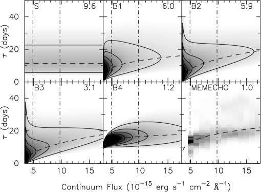
Figure 7: Luminosity-dependent delay maps for the 5 parameterized models as well as the MEMECHO recovered delay map. The reduced $\chi^{2}$ value of each fit is indicated. For the parameterized models, the dashed line indicates the dependence of the peak of the delay map on the continuum flux. For the MEMECHO model the dashed line indicates the best fit power-law, $\tau\propto F_{opt}^{\beta}$ to the delay map. The dot-dashed lines indicate the minimum and mean continuum flux of the 13-year data, and the upper-limit of the plots is the maximum continuum flux. The lower limit of the plots is the background continuum flux. Solid lines mark the contours of the delay map. The parameters for each model are shown in Table 2.

Table 2: Parameters for fits to 1989-2001 H$\beta$ lightcurve of NGC 5548. In all models the mean optical continuum level $\overline{F_{opt}}=9.73\times 10^{-15}$ erg s^-1 cm^-2 $\mathrm{\AA}^{-1}$.

	$\chi^{2}/1248$	$\alpha$	$\beta$	$\gamma$	$\overline{\tau_{0}}$	$\overline{\Delta\ln\tau}$	$\overline{F_{H\beta}}$	$\overline{\Psi_{0}}$
S	9.6	$1.0$	$0.0$	$0.0$	$11.4\pm 0.6$	$0.66\pm 0.05$	$7.67\pm 0.02$	$0.79\pm 0.01$
B1	6.0	$0.66\pm 0.03$	$0.28\pm 0.05$	$0.0$	$12.9\pm 1.0$	$0.70\pm 0.07$	$7.98\pm 0.02$	$0.77\pm 0.05$
B2	5.9	$0.57\pm 0.02$	$0.41\pm 0.08$	$-0.20\pm 0.06$	$13.9\pm 0.8$	$0.56\pm 0.05$	$7.98\pm 0.02$	$0.68\pm 0.01$
B3	3.1	$0.58\pm 0.03$	$0.46\pm 0.07$	$-0.24\pm 0.06$	$12.3\pm 0.7$	$0.58\pm 0.04$	$7.97\pm 0.01$	$0.68\pm 0.01$
B4	1.2	$0.64\pm 0.01$	$0.10\pm 0.01$	$0.46\pm 0.05$	$16.4\pm 0.3$	$0.32\pm 0.02$	$8.05\pm 0.01$	$0.68\pm 0.01$

Figure 8: Continuum and H$\beta$ lightcurves for 1991 - 1992 (left) and 1998 - 1999 (right). The linearly interpolated continuum flux model is marked with a solid line. The fit to the H$\beta$ lightcurve can be seen for 3 of the different models (B3 (solid line), B2 (dotted line) and S (dot-dashed line)).

4 MEMECHO fit to the NGC 5548 AGN Watch 1989-2001 lightcurves

The echo mapping computer code MEMECHO (see Horne et al., 1991; Horne, 1994, for technical details) can allow luminosity-dependent delay maps to be made by means of a maximum-entropy deconvolution of Eq. 3. The maximum-entropy method finds the simplest positive image that fits the data, balancing simplicity, measured by entropy, and realism, measured, in this case, by $\chi^{2}$ (Horne, 1994).

The optical continuum lightcurve, $F_{opt}(t)$, must thread through the measured continuum fluxes, and the predicted H$\beta$ emission-line lightcurve, $F_{H\beta}(t)$, must similarly fit the measured line fluxes. In our fit to the data points we adjust the line background flux $\overline{F_{H\beta}}$, the continuum variations $F_{opt}(t)$, and the delay map $\Psi(\tau,F_{opt})$, we take $\overline{F_{opt}}$ as the median of the continuum data. The fit is required to have a reduced $\chi^{2}/N=1\pm\sqrt{2/N}$, where $N$ is the number of data points. We require this to hold for the line flux measurements, and also for the continuum flux measurements. The continuum is split into several flux levels (indicated in the lower panel of Fig. 9), and delay maps corresponding to each level are determined. When computing the convolution (Eq. 3) we linearly interpolate between these continuum levels to find the delay map that applies to the continuum flux at time $t-\tau$. Such an approach allows for fully non-linear line responses. Further details of this can be found in Horne (1994).

Fig. 9 shows the measured lightcurves and the MEMECHO fit. The greyscale (middle panel) shows the delay map at each time. Fig. 10 shows the luminosity-dependent delay map $\Psi(\tau,F_{opt})$ (greyscale) reconstructed from the observed lightcurves at each continuum level. The crosses indicate the median of the delay map and the dots indicate the upper and lower quartiles (see Tab. 3). The lower left panel projects the delay map along the time delay axis and thus indicates that the amplitude of the line response decreases with rising continuum level. The upper right panel gives the luminosity-averaged one-dimensional transfer function. At each continuum luminosity the range of delays is relatively narrow compared to the one-dimensional transfer function. As the luminosity rises, the mean delay increases. At minimum light the median delay is $\sim 13$ days, and this rises to $\sim 23$ days at maximum light. Fitting a power-law of the form $\tau\propto F_{opt}^{\beta}$ (with the galaxy background continuum removed) to the median time delay leads to $\beta=0.24\pm 0.08$.

In order to understand how robust the MEMECHO recovered luminosity-dependent delay map is we ran a short Monte-Carlo simulation. We generated ten sets of continuum and H$\beta$ lightcurves with the data points shifted by a Gaussian random number with a mean of zero and standard deviation equal to the uncertainty on that data point. Ten different delay maps were then recovered using these lightcurves. The delay maps recovered are all close to the original. Fig. 11 shows the ten realisations of the delay maps when the continuum flux is at the average of the low and high states (7.0 and $13.0\times 10^{-15}$ erg s^-1 cm^-2 $\mathrm{\AA}^{-1}$ respectively). This shows the possible range of uncertainties expected in the delay map.

Table 3: Time delay at the median, lower and upper quartile of the MEMECHO luminosity-dependent delay map for each continuum flux.

Continuum Flux	Median delay	Lower quartile	Upper quartile
(10-15 erg s-1 cm-2 $\mathrm{\AA}^{-1}$)	(days)	(days)	(days)
5.	13.	11.	15.
6.	15.	12.	17.
7.	16.	13.	18.
8.	16.	14.	19.
9.	17.	15.	20.
10.	19.	16.	22.
11.	19.	17.	24.
12.	20.	17.	25.
13.	20.	18.	28.
14.	20.	18.	29.
15.	20.	18.	26.
16.	21.	18.	26.
17.	23.	19.	28.

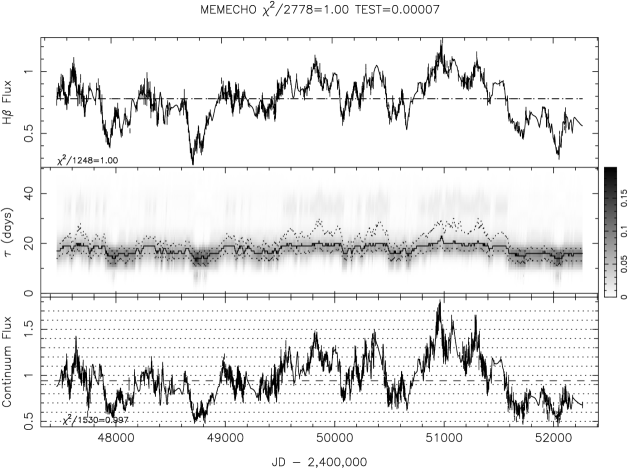
Figure 9: Lightcurves for optical continuum (bottom) and H$\beta$ emission line flux (top) from the 1989-2001 AGN Watch data on NGC 5548. The MEMECHO fit is the smoothest model that achieves $\chi^{2}/N=1\pm\sqrt{2/N}$ for both lightcurves. In the middle panel, the greyscale shows the delay map at each time, the solid line marks the median of the delay map, where as the dotted lines mark the lower and upper quartiles. The horizontal dotted lines in the bottom panel show the flux levels at which each delay map is determined.

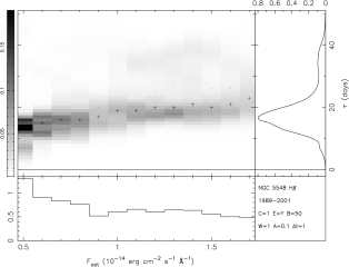
Figure 10: The luminosity-dependent delay map $\Psi(\tau,F_{opt})$ from the MEMECHO fit to the 1989-2001 AGN Watch data on NGC 5548.

Figure 11: 10 realisations of the MEMECHO recovered delay map at low and high continuum levels (7.0 and $13.0\times 10^{-15}$ erg s^-1 cm^-2 $\mathrm{\AA}^{-1}$ respectively) from Monte-Carlo simulations.

5 Discussion

Both the parameterized fit and the MEMECHO fit to the 13-year continuum and H$\beta$ lightcurves for NGC 5548 show that H$\beta$ reverberations depend upon the continuum state in such a way that greater time delays occur for higher continuum states. From the parameterized breathing models we find that $\tau\propto F_{opt}^{\beta}$ with $\beta$ in the range 0.1 to 0.46, depending on the specific model, with the continuum at 5100 $\rm{\AA}$ corrected for the galaxy contribution. However, as noted in $\S$2.2, the driving ionizing continuum may be closer to that observed at 1350 $\rm{\AA}$. Using our relationship that $F_{opt}\propto F_{UV}^{0.53}$, the luminosity-dependent lag scales like $\tau\propto F_{UV}^{0.05-0.24}$. The MEMECHO fit gives $\tau\propto F_{opt}^{0.24}$, or $\tau\propto F_{UV}^{0.13}$ with respect to the UV continuum. This would appear to be in contrast with both the results of the Static model fits to the separate years, where we find $\tau\propto F_{opt}^{0.93}$, and the findings of Peterson et al. (2002) where they find that CCF centroid lag scales as $F_{opt}^{0.95}$. Our values from the breathing models are closer to that predicted by the photoionization models of Korista & Goad (2004) who find that the responsivity weighted radius, $R\propto F_{c}^{0.23}$, although they noted that the power-law slope should differ somewhat in high (flatter) and low (steeper) continuum states.

Peterson et al. (2002) determine the lag on a yearly basis using cross-correlation. As mentioned in $\S$ 2, the CCF is the convolution of the delay map with the ACF. Thus, it is clear that the time delay between the line and continuum light curves determined via cross-correlation depends on the shape of both the delay map and the ACF of the continuum. If the ACF is a delta function, then the CCF is identical to the delay map. Generally the ACF is broad and the delay map is asymmetric, thus the peak of the CCF will not necessarily occur at the same time delay as in the delay map (e.g. Welsh, 1999). The continuum variability properties of NGC 5548 vary from year to year leading to a change in ACF, and as an artifact of this, a change in lag could be measured without there being a change in the delay map. It is also the case that the accuracy of the CCF centroid depends on the length of the sampling window, the sampling rate, the continuum variability characteristics and the data quality (Perez et al., 1992). Throughout the 13-year monitoring campaign of NGC 5548 the mean sampling rate has varied, which could lead to a change in the determined lag. However, our results from the Static fits to the yearly data produce similar lags (when comparing our $\tau_{med}$ with the centroid lag) and a similar slope to Peterson et al. (2002), suggesting that the cross-correlation results may be measuring the true lags.

Both the parameterized breathing fits and the MEMECHO fit to the full 13-year data show a much flatter dependence of the lag on the luminosity than the year-by-year analysis shows. There is scatter within the results from the yearly analysis. For example, there is a wide range of delay ($\sim 9-18$ days) when the continuum is in a low state with $F_{opt}\sim 7\times$10^-15 erg s^-1 cm^-2 $\mathrm{\AA}^{-1}$, and there is also a wide range of continuum fluxes (7 - 12$\times$10^-15 erg s^-1 cm^-2 $\mathrm{\AA}^{-1}$) that have a lag of approximately 17 days. A wide range of delays at low continuum flux and also the same lag at a wide range of fluxes favours a flatter relationship. It could be that these features dominate over the two years with the largest lag when fitting to the full 13-year data set. The tail to long delays on the delay maps determined by the parameterized models and the MEMECHO fits may also allow a flatter relationship. The difference in slope is certainly interesting and merits further investigation.

From both the parameterized models and the MEMECHO fits, we also find that the amplitude of the H$\beta$ response declines with increasing continuum luminosity, in other words, the change in H$\beta$ flux relative to changes in the continuum is greater in lower continuum states. Detailed photoionization calculations by Korista & Goad (2004) predict this, and Gilbert & Peterson (2003) and Goad et al. (2004) find the same general result. From our parameterized fits to the data, we find $F_{H\beta}\propto F_{opt}^{\alpha}$ with $0.57<\alpha<0.66$, which is consistent with that found by Gilbert & Peterson (2003). Correcting our relationship to be relative to the UV continuum gives $F_{H\beta}\propto F_{UV}^{0.30-0.35}$, which is close to the relationship shown in Fig 2 (c). Goad et al. (2004) find a range in this parameter (relative to the optical continuum) of $0.41<\alpha<1.0$, that correlates with the optical continuum flux with a high degree of statistical confidence. Korista & Goad (2004) find this to be a natural result, given that the H$\beta$ equivalent width drops with increasing incident photon flux. Their model predicts slightly higher values for the responsivity to the ionizing flux ($F_{H\beta}\propto F_{ion}^{0.54-0.77}$) than we observe from the parameterized fits.

The MEMECHO recovered delay map (Fig. 7, panel (f) and Fig. 10) and the delay map from the B4 model (Fig. 7, panel (e)) seem similar, which is not suprising as they are both driven by the same continuum lightcurve model. However, the B4 model differs from the B1, B2, and B3 models, particularly in its value for $\beta$, because of the differing continuum models used. MEMECHO allows the continuum model to have more freedom between the data points (compared to the linear interpolation used in models B1 - B3) resulting in a delay map with a smaller width at shorter time delays as less blurring of the continuum lightcurve is required. Nevertheless, the $\alpha$ parameter does not vary too much between the different models. It is also interesting to note that the residuals in B4 are very flat, even without the spline fit, the long term trends seen in the residuals to B2 have disappeared. On close inspection of the MEMECHO fit to the continuum (see Fig. 12), it can be seen that between the data points the continuum model sometimes shows unphysical dips and peaks. For instance, if the model constantly dips down between the data points, the lag between the continuum and the line lightcurves can be shifted without altering the delay map. In this way it seems that MEMECHO accounts for the long timescale variations that cannot be described by the delay map in the B2 model. Although these spurious dips mean that the MEMECHO result may not be completely reliable, it is clear that the recovered lag luminosity relationship is much flatter than found by the cross-correlation method and thus is an important independent check of the parameterized models.

Figure 12: A section of the MEMECHO fit to the continuum lightcurve covering the observing campaign in 1993 and 1994.

For the B3 and B4 models we allowed a spline fit to the residuals to account for slowly varying trends (timescale $\sim$ 1 year, see Fig. 6). We suggest that these long timescale variations are not due to reverberation effects, but due to slow changes of the BLR gas distribution. In a study of the line profile variability of the first five years of the AGN Watch data on NGC 5548, Wanders & Peterson (1996) find that although the H$\beta$ emission line flux tracks the continuum flux, the H$\beta$ emission line profile variations do not, and therefore are not reverberation effects within the BLR. In Fig. 13 we compare the line profile ‘shapes’ determined by Wanders & Peterson (1996) for the first five years of data with our residuals from the B2 model. Wanders & Peterson (1996) define these emission-line ‘shapes’ to describe the relative prominence of features in the emission-line profile. Each profile is split into its red wing, core and blue wing and the ‘shape’ for each determined. A positive number for the shape indicates that it is more prominent than on average, whereas a negative number indicates that it is less prominent than on average. Although the shapes vary on similar timescales to the residuals, there is no obvious correlation with the profile shape variations. A comparison of the profile variability for the full 13-year data with our residuals warrants further study.

Figure 13: A comparison of the ‘shapes’ of the red wing, blue wing and core of the H$\beta$ line profile as calculated by Wanders & Peterson (1996) with the residuals of the B2 parameterized model, and the continuum and H$\beta$ flux with the B2 model shown.

6 Conclusion

Our analysis of 13 years of optical spectrophotometric monitoring of the Seyfert 1 galaxy NGC 5548 from 1989 through 2001 reveals that the size of the H$\beta$ emission-line region increases as the continuum increases. Will also find that the strength of the H$\beta$ response decreases with increasing continuum flux. We have fit the H$\beta$ emission-line lightcurve using both parameterized models and the echo-mapping code MEMECHO, both methods show these effects.

In our parameterized models, we allow the delay map to be luminosity-dependent. Our model is parameterized such that the H$\beta$ emission can respond non-linearly to the optical continuum variations, i.e., $F_{H\beta}\propto F_{opt}^{\alpha}$. From our fits to the data we determine $0.57<\alpha<0.66$ which is consistent with previous findings of Gilbert & Peterson (2003) and Goad et al. (2004). However, the ionizing continuum is likely to be closer to the UV continuum ($F_{UV}$) than the optical continuum. Correcting for this ($F_{opt}\propto F_{UV}^{0.53}$) gives $F_{H\beta}\propto F_{UV}^{0.30-0.35}$. In addition, we allow the peak of the delay map, $\tau_{0}$, to be luminosity-dependent, $\tau_{0}\propto F_{opt}^{\beta}$, and find $0.10<\beta<0.46$. Correcting to be with respect to the UV continuum gives $\tau_{0}\propto F_{UV}^{0.05-0.24}$. MEMECHO fits to the lightcurves also show these effects, and fitting a power-law of the form $\tau\propto F_{opt}^{\beta}$ to the luminosity-dependent delay map gives $\tau\propto F_{opt}^{0.24}$, or $\tau\propto F_{UV}^{0.13}$. The values we determine for $\beta$ (corrected to be relative to the UV continuum) are not consistent with the simple Strömgren sphere ($\beta=1/3$) and ionization parameter ($\beta=1/2$) arguments and have a flatter slope than the $\beta=0.95$ result from the cross-correlation analysis of Peterson et al. (2002). However, they are close to the prediction of Korista & Goad (2004) whose more detailed photoionization models predict $\beta=0.23$.

In our parameterized models we find slowly vary residuals (timescale $\sim$ 1 year) which we suggest are not reverberation effects, but indicate changes in the gas distribution. Comparison of these residuals with velocity profile changes from the first five years of the data (Wanders & Peterson, 1996) are inconclusive. In future work we will examine velocity profile changes of the full 13-year lightcurves.

Acknowledgements

EMC is supported by a PPARC Studentship at the University of St Andrews. EMC wishes to thank Mike Goad and Kirk Korista for very useful discussions about this work during a visit to the University of Southampton. The authors would also like to thank Kirk Korista, Brad Peterson and the referee, Andrew Robinson, for comments which have improved the manuscript.

References

- Baldwin et al. (1995) Baldwin J., Ferland G., Korista K., Verner D., 1995, ApJ, 455, L119
- Baldwin (1977) Baldwin J. A., 1977, ApJ, 214, 679
- Blandford & McKee (1982) Blandford R. D., McKee C. F., 1982, ApJ, 255, 419
- Clavel et al. (1991) Clavel J., et al., 1991, ApJ, 366, 64
- Dietrich & Kollatschny (1995) Dietrich M., Kollatschny W., 1995, A&A, 303, 405
- Gaskell & Peterson (1987) Gaskell C. M., Peterson B. M., 1987, ApJS, 65, 1
- Gaskell & Sparke (1986) Gaskell C. M., Sparke L. S., 1986, ApJ, 305, 175
- Gilbert & Peterson (2003) Gilbert K. M., Peterson B. M., 2003, ApJ, 587, 123
- Goad et al. (2004) Goad M. R., Korista K. T., Knigge C., 2004, MNRAS, 352, 277
- Horne (1994) Horne K., 1994, in ASP Conf. Ser. 69: Reverberation Mapping of the Broad-Line Region in Active Galactic Nuclei Echo Mapping Problems Maximum Entropy solutions. pp 23–25
- Horne et al. (1991) Horne K., Welsh W. F., Peterson B. M., 1991, ApJ, 367, L5
- Kinney et al. (1990) Kinney A. L., Rivolo A. R., Koratkar A. P., 1990, ApJ, 357, 338
- Korista et al. (1995) Korista K. T., et al., 1995, ApJS, 97, 285
- Korista & Goad (2004) Korista K. T., Goad M. R., 2004, ApJ, 606, 749
- Krolik et al. (1991) Krolik J. H., Horne K., Kallman T. R., Malkan M. A., Edelson R. A., Kriss G. A., 1991, ApJ, 371, 541
- Netzer & Maoz (1990) Netzer H., Maoz D., 1990, ApJ, 365, L5
- O’Brien et al. (1995) O’Brien P. T., Goad M. R., Gondhalekar P. M., 1995, MNRAS, 275, 1125
- Osmer et al. (1994) Osmer P. S., Porter A. C., Green R. F., 1994, ApJ, 436, 678
- Perez et al. (1992) Perez E., Robinson A., de La Fuente L., 1992, MNRAS, 255, 502
- Peterson (1993) Peterson B. M., 1993, PASP, 105, 247
- Peterson et al. (1999) Peterson B. M., et al., 1999, ApJ, 510, 659
- Peterson et al. (2002) Peterson B. M., et al., 2002, ApJ, 581, 197
- Peterson et al. (2004) Peterson B. M., et al., 2004, ApJ, 613, 682
- Pogge & Peterson (1992) Pogge R. W., Peterson B. M., 1992, AJ, 103, 1084
- Robinson & Perez (1990) Robinson A., Perez E., 1990, MNRAS, 244, 138
- Romanishin et al. (1995) Romanishin W., et al., 1995, ApJ, 455, 516
- Wanders & Peterson (1996) Wanders I., Peterson B. M., 1996, ApJ, 466, 174
- Welsh (1999) Welsh W. F., 1999, PASP, 111, 1347
- White & Peterson (1994) White R. J., Peterson B. M., 1994, PASP, 106, 879